Confidential direct communications: a quantum approach using continuous variables

Let us consider a bosonic mode with Hilbert space $\mathcal{H}$ and ladder operators $\hat{a},\hat{a}^{\dagger}$ satisfying $[\hat{a},\hat{a}^{\dagger}]=1$. Equivalently, this system can be described by a pair of quadrature operators

satisfying the dimensionless canonical commutation relation (CCR) $[\hat{q},\hat{p}]=i$. From the previous CCR we see that an arbitrary state of the system $\rho$ must fulfill the uncertainty principle

where $V(\hat{x}):=\mathrm{Tr}(\rho\hat{x}^{2})-[\mathrm{Tr}(\rho\hat{x})]^{2}$ denotes the variance of an arbitrary quadrature $\hat{x}=\hat{q}$ or $\hat{p}$. In particular, an arbitrary coherent state $|\bar{\alpha}\rangle$ saturates Eq. (2) symmetrically, i.e., $V(\hat{q})=V(\hat{p}):=\Delta=1/2$, where the value $1/2$ quantifies the so-called quantum shot-noise. This is the fundamental noise that affects the disjoint measurements of the quadratures $\hat{q}$ and $\hat{p}$ of a coherent state (via homodyne detection [9]). Such a noise is instead doubled to $\Delta=1$ when the two quadratures are measured jointly (via heterodyne detection [9]).

According to the Wigner representation, an arbitrary density operator $\rho$ is equivalent to a characteristic function $\chi(\lambda):=\mathrm{Tr}[\rho\hat{D}(\lambda)]$, where $\hat{D}(\lambda):=\exp(\lambda\hat{a}^{\dagger}-\lambda^{\ast}\hat{a})$ is the displacement operator. Equivalently, $\rho$ can be described by a Wigner function, which is a quasi-probability distribution defined by the Fourier transform

In Eq. (3), the Cartesian decomposition of the complex variable $\alpha=(q+ip)/\sqrt{2}$ provides the real eigenvalues $q$ and $p$ of the quadrature operators of Eq. (1). Such variables span the phase-space $\mathcal{K}=\{q,p\}$ of the system and, therefore, represent its fundamental continuous variables. For a coherent state $|\bar{\alpha}\rangle$, the Wigner function takes the form

where

is a complex Gaussian function with mean $\bar{\alpha}$ and variance $V$. As a consequence, the measurement of the arbitrary quadrature $\hat{x}$ provides outcomes $x$ which are distributed according to the real Gaussian

where $\Delta=1/2$ for homodyne detection, while $\Delta=1$ for heterodyne detection.

Let us discretize the phase-space $\mathcal{K}$ by introducing a square lattice whose unit cell has size equal to $2\Omega$ (see Fig. 1). An arbitrary cell can be addressed by a pair of integer indices $(u,u^{\prime})$ and its center specified by the coordinates

or, equivalently, by the complex amplitude

Thanks to the introduction of this discrete structure, two bits of information may be simply encoded in quantum phase-space. In fact, an arbitrary cell of address $(u,u^{\prime})$ can be associated with a pair of bits $(U,U^{\prime})$, representing the parities of the indices $u$ and $u^{\prime}$. In this approach, Alice encodes two classical bits $(U,U^{\prime})$ by choosing a cell whose address $(u,u^{\prime})$ is randomly selected according to the relations

where $m$ and $m^{\prime}$ are random integers [10]. Then, she considers the complex amplitude $\alpha_{uu^{\prime}}$ pointing at the center of that cell and prepares a corresponding coherent state $|\alpha_{uu^{\prime}}\rangle$. Such a state is finally sent to Bob, who performs a heterodyne detection in order to estimate the amplitude $\alpha_{uu^{\prime}}$ and therefore the encoded information $(U,U^{\prime})$. It is clear that, even in the presence of a noiseless communication channel, Bob’s decoding cannot be noiseless since the Gaussian shape of the coherent state spreads over the whole of phase space. Such a spread inevitably leads to an intrinsic error in the decoding process which occurs when the coherent state is projected by the measurement to wrong peripheral cells.

Let us evaluate the probability $\varepsilon$ of an intrinsic error when Bob decodes Alice’s bit $U$ from the position quadrature $\hat{q}$ (the argument may be repeated for the other quadrature). Since Bob performs a heterodyne detection on the coherent state, the measured value $q$ will be distributed around $q_{u}$ according to a Gaussian distribution with noise-variance equal to $\Delta=1$, i.e., $G_{1}(q-q_{u})$. Suppose, for simplicity, that $U=0$ is encoded in $q_{u}=0$. According to Fig. 2 an error occurs whenever the measured value $q$ falls in one of the crossed cells, i.e., having odd index $u=\pm 1,\pm 3,...$ (which would lead to the incorrect reconstruction of $U=1$ by Bob). Hence, the probability of an intrinsic error (per quadrature) is equal to

Now, if we fix a tolerable value for the intrinsic error probability, we find the corresponding size $\Omega$ to be used for the lattice. In particular, tolerating $\varepsilon=1\%$ implies adopting $\Omega\simeq 2.57$. On the one hand, the use of a low value for $\varepsilon$ enables the honest users to approach noise-free communication. On the other hand, a large value for $\Omega$ makes the protocol particularly fragile to eavesdropping. In fact, Eve can optimize her attack on the structure of the lattice, e.g., by using a non-universal cloner which is optimized on the centers of the cells. More simply, Eve can detect the state, reconstruct its cell, and resend another state which is centered in that cell. By resorting to this intercept-center-resend strategy, Eve is able to remove the noise most of the time for a sufficiently large $\Omega$. Luckily, we are able to preclude such strategies by resorting to the classical procedure shown in the next section.

In order to hide the lattice from Eve, Alice can simply add a mask to her message. After the computation of the message amplitude $\alpha_{uu^{\prime}}$, Alice classically adds a mask amplitude $\alpha_{M}$, in such a way that the total amplitude $\bar{\alpha}:=\alpha_{M}+\alpha_{uu^{\prime}}$ is randomly distributed according to a complex Gaussian $\mathcal{G}_{V}(\bar{\alpha})$ with large variance $V\gg\Omega$ (see Fig. 1). Operationally, the whole encoding procedure goes as follows:

(1) Lattice Encoding.

Alice encodes the message bits $(U,U^{\prime})$ into a message amplitude $\alpha_{uu^{\prime}}$.

(2) Masking.

Alice picks a signal amplitude $\bar{\alpha}$ from a wide Gaussian distribution and computes the mask $\alpha_{M}=\bar{\alpha}-\alpha_{uu^{\prime}}$ connecting signal and message.

(3) Quantum Preparation.

Alice prepares a signal coherent state $\left|\bar{\alpha}\right\rangle$ to be sent to Bob.

Clearly, the same decoding steps can be followed by Eve too. However, the key point is that Eve must choose the probing interaction before knowing the value of the mask. Since the signal $\bar{\alpha}$ is continuous (Gaussian) and highly modulated, Eve is prevented from using any kind of interaction which privileges a particular portion of the phase space. The most natural choice is therefore a universal Gaussian interaction. A possible model is given by the universal Gaussian quantum cloning machine (UGQCM) [12]. Such a machine maps the signal state $\left|\bar{\alpha}\right\rangle$ into a pair of output clones $\rho_{B}$ (sent to Bob) and $\rho_{E}$ (taken by Eve), each one equal to a Gaussian modulation of $\left|\bar{\alpha}\right\rangle\left\langle\bar{\alpha}\right|$, i.e.,

where the cloning-noise variances $\sigma_{B}^{2}$ and $\sigma_{E}^{2}$ symmetrically affect the quadratures and satisfy the optimality condition

directly imposed by Eq. (2) [13]. As a consequence of Eq. (11), the arbitrary quadrature $\hat{x}$ of the clone $K=B,E$ has a marginal distribution equal to $G_{\Delta+\sigma_{K}^{2}}(x-\bar{x})$. The performance of the resulting attack will be explicitly studied in the next Section II.4.

The above procedure of directly communicating message bits is called the message mode (MM) of the protocol. However, Alice and Bob must also understand how much the channel is perturbed during the communication process, in order to control the amount of information which is left to a potential eavesdropper. Assuming an attack with UGQCM, this corresponds to estimating the value of the noise $\sigma_{B}^{2}:=\sigma^{2}$ which is added by Eve to the channel. A real-time check of this noise is possible if Alice randomly switches from instances of message mode to suitable instances of control mode (CM). In control mode, Alice does not process any text message but only prepares and sends the signal state $\left|\bar{\alpha}\right\rangle$ (see Fig. 4). Then, after Bob’s detection (outcome $\beta$), Alice communicates the value $\bar{\alpha}$ of the signal amplitude. At that point, Bob extracts from $(\beta,\bar{\alpha})$ the actual value of the test variable $\tau:=\beta-\bar{\alpha}$ which is then used to infer the total noise $\Delta_{B}=1+\sigma^{2}$ affecting the signal. As soon as they recognize a non-tolerable noise, i.e., $\sigma^{2}>\tilde{\sigma}^{2}$ for some threshold noise $\tilde{\sigma}^{2}$, they stop the communication. Hereafter, we assume a zero-tolerance protocol where no added noise is tolerated on the channel, i.e., $\tilde{\sigma}^{2}=0$. We shall see that the QDC protocol can be applied in realistic situations even with such a strict condition [14].

Let us show how the real-time check of the quantum channel works in detail. Let us consider the Cartesian decomposition $\tau=(q+ip)/\sqrt{2}$ of Bob’s test variable. If the channel is noiseless, then the arbitrary quadrature $x=q$ or $p$ is only affected by heterodyne noise $\Delta=1$, i.e., it is distributed according to a Gaussian distribution $G_{1}(x)$. By contrast, if Eve perturbs the quantum channel using a UGQCM with noise $\sigma^{2}\neq 0$, then $x$ follows a wider Gaussian distribution $G_{1+\sigma^{2}}(x)$. By reconstructing the experimental distribution of $x$ from consecutive outcomes $\{x_{1},x_{2},\cdots\}$, Bob must therefore distinguish between the two theoretical distributions $G_{1}(x)$ and $G_{1+\sigma^{2}}(x)$. In other words, Bob must distinguish between the two hypotheses

Let us fix the confidence level $r$ of this hypothesis test, i.e., the probability to reject $H_{0}$ though it is true. This level must be sufficiently low (e.g., $r=5\times 10^{-7}$), so that the direct communication can be effectively completed in absence of Eve. For each instance of control mode, Bob makes two independent tests, one for each quadrature. Hence, after $M$ control modes, he has collected $2M$ quadratures values $\{q_{1},p_{1},\cdots,q_{M},p_{M}\}:=\{x_{1},x_{2},\cdots,x_{2M-1},x_{2M}\}$ and he can construct the estimator

Then, the hypothesis $H_{0}$ is accepted if and only if

where $\mathcal{V}_{i,j}$ is the $j$th quantile of the $\chi^{2}$ distribution with $i$ degrees of freedom. In other words, Alice and Bob continue their direct communication in MM as long as the condition of Eq. (15) is satisfied in CM.

Let us explicitly analyze what happens when the quantum communication channel is subject to Gaussian eavesdropping via a UGQCM. In an individual UGQCM attack (see Fig. 5), Eve clones the signal input and, then, heterodynes her output to derive her estimate $\gamma$ of the signal amplitude $\bar{\alpha}$. After the release of the mask’s value $\alpha_{M}$, Eve infers the message amplitude $\alpha_{uu^{\prime}}$ and, therefore, the input bits $(U,U^{\prime})$. In this process, Eve introduces an added noise $\sigma^{2}$ on the Alice-Bob channel (i.e., $\Delta_{B}=1+\sigma^{2}$), while her output is affected by a total noise equal to $\Delta_{E}=1+(4\sigma^{2})^{-1}$. This is the sum of the cloning noise $\sigma_{E}^{2}=(4\sigma^{2})^{-1}$, given by the UGQCM, and the measurement noise $\Delta=1$, given by the heterodyne detector.

First of all, we must evaluate the probability of accepting $H_{0}$ (hence continuing the communication) notwithstanding the presence of Eve. In other words, we must compute the probability $\Pi_{M}(\sigma^{2})$ that Eve evades $M$ control modes while introducing a noise $\sigma^{2}\neq 0$. After $M$ control modes, the estimator of Eq. (14) follows the distribution

As a consequence, the probability to accept $H_{0}$ is equal to

where

is the incomplete gamma function.

Besides Eve’s survival probability of Eq. (17), we must also evaluate the amount of information that Eve can get during her undetected life on the channel. Such a quantity is limited by the total noise experienced by Eve, which is equal to $\Delta_{E}=1+(4\sigma^{2})^{-1}$. For a given $\Delta_{E}$, we now calculate the average information Eve can steal in a single run of MM. Starting from the outcome of the measurement $\gamma$ and the knowledge of the mask $\alpha_{M}$, Eve estimates Alice’s amplitude $\alpha_{uu^{\prime}}$ via the variable $\gamma-\alpha_{M}$. The corresponding quadrature $x$ will be distributed according to a Gaussian distribution $G_{\Delta_{E}}(x-x_{u})$. Then, by repeating the same derivation leading to Eq. (10), we can compute Eve’s error probability in decoding Alice’s bit ($U$ or $U^{\prime}$), which is equal to

Let us assume that every message bit is a bit of information, i.e., the input message is not compressible. As a consequence, the average amount of information which is eavesdropped in a single MM is given by

where

By replacing $\Delta_{E}=1+(4\sigma^{2})^{-1}:=\Delta_{E}(\sigma^{2})$ in Eq. (20), we derive $I_{AE}=I_{AE}(\sigma^{2})$, i.e., the average amount of information which is stolen for a given noise $\sigma^{2}$ in Alice-Bob channel. Such a quantity can be directly combined with $\Pi_{M}=\Pi_{M}(\sigma^{2})$ of Eq. (17). This means that we can express Eve’s survival probability as a function of the stolen information. In fact, let us fix the probability $c$ of a control mode, so that $N$ runs of the protocol can be divided into $cN$ control modes and $(1-c)N$ message modes, on average. As a consequence, Eve’s survival probability is equal to

and the average number of stolen bits is equal to

Then, for every $\sigma^{2}$, we can consider the function $P=P(I)$. In particular, let us fix $c=69/70$, so that the protocol has efficiency

For several values of $\sigma^{2}$, we can (numerically) evaluate the function $P=P(I)$ as shown in Fig. 6. From this figure, we can see that, if the noise is low, e.g., $\sigma^{2}=0.01$, Eve steals very little information ($\simeq 1$ bit) while Alice and Bob complete an almost noiseless QDC. In particular, Alice is able to transmit $\simeq 1.5\times 10^{4}$ bits of information by using $N\simeq 5\times 10^{5}$ systems. Notice that the maximum length of the QDC is roughly bounded by the verification of $r^{-1}$ hypothesis tests and, therefore, it is limited to about $4(1-c)(cr)^{-1}$ bits (i.e., $\simeq 1.2\times 10^{5}$ bits or $\simeq 4\times 10^{6}$ systems using the above parameters). If the attack is more noisy (e.g., $\sigma^{2}=1$), Eve again steals little information ($\simeq 1$ bit). In such a case, in fact, Eve is promptly detected by the honest parties who, however, are prevented from exchanging information (denial of service). According to Fig. 6, Eve’s best strategy corresponds to using a UGQCM with $\sigma^{2}\simeq 1/20$, so that she can steal a maximal amount of about $80$ bits before being revealed (using a cut off of $P=1\%$). In such a case, Alice transmits $\simeq 630$ bits by using $N\simeq 2.2\times 10^{4}$ systems.

How can we decrease the maximal amount of stolen information? The simplest solution consists in increasing the control mode probability $c$, so that the possible presence of Eve is detected before sending too many bits. Clearly, this approach has a price to pay, which is a decrease of the efficiency $\mathcal{E}$ of the protocol. An alternative solution consists of making the decoding more sensitive to the presence of added noise. Such an approach is possible by introducing classical error correcting codes, and its pros and cons are explored in the following section. In particular, this solution is good against Gaussian attacks but its advantages are not completely clear in the presence of non-Gaussian attacks.

In the basic scheme of QDC with continuous variables, a noiseless communication is possible up to an intrinsic error probability $\varepsilon$ which depends on the step $\Omega$ of the phase-space lattice. In particular, such a probability decreases for increasing $\Omega$. An alternative way for decreasing $\varepsilon$ consists of leaving $\Omega$ unchanged while introducing a classical error correcting code for encoding/decoding. Such procedures are equivalent for a noiseless channel, since $\varepsilon$ is sufficiently small and the codes work very well in that case. However, the scenario is different as the channel becomes nosier. In such a case, in fact, the correcting codes have a non-linear behavior which makes their performance rapidly deteriorate. Such a non-linear effect can be exploited to critically split the correction capabilities, and therefore the information gains, between Alice-Bob channel and Alice-Eve channel.

Let us consider the simple case of an $n$-bit repetition code, where an input bit $U=\{0,1\}$ is encoded into a logical bit $\bar{U}=\{\bar{0},\bar{1}\}$ of $n$ physical bits via the codewords

By choosing an odd $n=2m+1$ (with $m=1,2,\cdots$), we can apply a non-ambiguous majority voting criterion. This means that every bit-flip error of weight $t<m+1$ is correctable, while every bit-flip error of weight $t\geq m+1$ is not. Let us now consider a memoryless channel, where each physical bit is perturbed independently with the same bit-flip probability $p$, as happens in the case of individual Gaussian attacks. Then, the probability of an uncorrectable error is simply given by

As it is evident from Fig. 7, the correction capability of the $n$-bit repetition code rapidly worsens as the single bit-flip probability approaches $1/2$. This is due to the non-linear behavior of $P_{n}=P_{n}(p)$ which becomes more manifest when $n$ increases. In particular, for a sufficiently large $n$, the curve displays a critical point $\tilde{p}$ after which the correction capability suddenly starts to deteriorate very quickly (e.g., $\tilde{p}\simeq 0.3$ for $n=35$ and $\tilde{p}\simeq 0.4$ for $n=103$). Exactly these critical points can be exploited to improve the QDC, by transforming the communication protocol into a threshold process, where the sensitivity to added noise is remarkably amplified.

For a repetition code of fixed length $n$, we have a corresponding critical value $\tilde{p}$. Then, we can choose a lattice whose step is critical. This is the value $\tilde{\Omega}$ such that the intrinsic error probability is critical, i.e., $\varepsilon(\tilde{\Omega})=\tilde{p}$. On the one hand, when the channel is noiseless, Bob is able to recover the codewords and reconstruct the logical bit with a very low error probability $P_{B}=P_{n}(\tilde{p})$. On the other hand, when the channel is noisy, Alice’s information is split into two sub-channels: the Alice-Bob channel, with added noise $\sigma_{B}^{2}:=\sigma^{2}$, and the Alice-Eve channel, with added noise $\sigma_{E}^{2}=(4\sigma^{2})^{-1}$. The corresponding error probabilities are respectively given by

where $p_{B}=p_{B}(\sigma_{B}^{2})$ and $p_{E}=p_{E}(\sigma_{E}^{2})$ are monotonic functions of the added noises (and, therefore, linked by the uncertainty principle). Now, if Eve tries to hide herself by perturbing the Alice-Bob channel with a relatively small $p_{B}$, then her dual $p_{E}$ will always be big enough to perturb $\tilde{p}$ into the nonlinear region. As a consequence, Eve will tend to experience $P_{E}\simeq 1/2$ gaining her negligible information.

Let us explain the previous point in terms of mutual information. In particular, let us fix the repetition code to the value $n=35$, so that we have $\tilde{p}\simeq 0.3$ and a corresponding critical value $\tilde{\Omega}\simeq 1$ for the lattice. Starting from an arbitrary $\Omega$, one can see that $\tilde{\Omega}$ is indeed optimal for Alice and Bob. For every bit of information which is encoded by Alice, the amount of information decoded by Bob and Eve is respectively given by

where $P_{B}$ and $P_{E}$ are the logical error probabilities in Eq. (27) with $n=35$. Since the added noises satisfy the uncertainty relation of Eq. (12), a similar relation holds for the mutual informations, i.e.,

where $\mu(\Omega,\sigma^{2})\leq 2$ is numerically shown in Fig. 8. Let us also consider the difference of information

Such a quantity is a point-by-point measure of how much $I_{AB}$ and $I_{AE}$ are different. In particular, the maximum value $D=1$ corresponds to the maximal separation $\{I_{AB},I_{AE}\}=\{0,1\}$ or $\{1,0\}$. As we can see from Fig. 9, the points $(\Omega,\sigma^{2})$ with $\Omega=1$ (i.e., with $\Omega\simeq\tilde{\Omega}$) corresponds to the broadest areas of separation. In other words, the critical condition $\Omega\simeq\tilde{\Omega}$ enhances the split between $I_{AB}$ and $I_{AE}$.

Let us explicitly show how to use an $n$-bit repetition code for encoding/decoding. This is possible by simply adding pre-encoding and post-decoding classical steps to the basic protocol of Sec. II. The message bits $(U,U^{\prime})$ are pre-encoded into a pair of logical bits

via the $n$-bit repetition code. Each pair of physical bits $(U_{k},U_{k}^{\prime})$ is then subject to the same encoding as before, i.e., lattice encoding $(U_{k},U_{k}^{\prime})\rightarrow\alpha_{u_{k}u_{k}^{\prime}}:=\alpha_{k}$, masking $\alpha_{k}\rightarrow\alpha_{k}+\alpha_{M}=\bar{\alpha}$ and quantum preparation $\bar{\alpha}\rightarrow\left|\bar{\alpha}\right\rangle$. Then, after $n$ message modes, Bob will have collected perturbed versions of the $n$ pairs $(U_{1},U_{1}^{\prime}),\cdots,(U_{n},U_{n}^{\prime})$. By applying standard error recovery (majority voting), he will then perform the post-decoding of $(U,U^{\prime})$. In the same way as before, these instances of message mode (each one carrying a single physical bit of a codeword) must be randomly switched with instances of control mode, where Alice skips encoding and simply sends Gaussian signals $\bar{\alpha}$ for testing the channel (exactly as in Fig. 4).

Let us choose a repetition code with $n=35$, and a lattice with $\Omega=1\simeq\tilde{\Omega}$. The latter choice implies an intrinsic error probability $\varepsilon$, in decoding the physical bits $(U_{k},U_{k}^{\prime})$, which is equal to the critical value of the code $\tilde{p}\simeq 32\%$. After error recovery, the intrinsic error probability $\bar{\varepsilon}$ affecting the logical bits $(\bar{U},\bar{U}^{\prime})$ is sufficiently low and corresponds to $P_{35}(\tilde{p})\simeq 1\%$. Then, let us also choose $c=1/2$ for the control mode’s probability, so that we have an efficiency $\mathcal{E}=1/35$. Notice that the values of $\bar{\varepsilon}$ and $\mathcal{E}$ correspond to the ones chosen for the basic protocol of Sec. II (where $\bar{\varepsilon}=\varepsilon$ of course). Such parameters equalize the performances of the two protocols in the case of noiseless quantum channel. As a consequence, we are in a situation to make a fair comparison between the protocols when malicious noise is present on the channel.

Let us analyze the effect of an individual UGQCM attack. On every cloned system, affected by a noise $\sigma_{E}^{2}=(4\sigma^{2})^{-1}$, Eve detects the complex amplitude $\gamma$ via heterodyne detection. Then, she estimates the signal amplitude $\bar{\alpha}$ up to a total noise $\Delta_{E}=1+\sigma_{E}^{2}$. After Alice’s declaration of the mask $\alpha_{M}$, Eve derives the message amplitude and, therefore, a pair of physical bits $(U_{k},U_{k}^{\prime})$. Each physical bit will be affected by an error probability $p(\Delta_{E})$ as in Eq. (19). After $n$ eavesdropped message modes, Eve will be able to decode Alice’s logical bits $(\bar{U},\bar{U}^{\prime})$ by majority voting, up to an error probability $P_{E}=P_{n}[p(\Delta_{E})]$ [see Eq. (26)]. For each logical bit, the acquired information is simply equal to $1-H(P_{E})$. As a consequence, for each message mode, Eve acquires on average

bits of information (simply because $2$ logical bits are sent via $n$ physical systems).

Now, let us consider the probability that Eve evades $M$ control modes. Since the control mode is implemented exactly as before, we have again $\Pi_{M}(\sigma^{2})$ as in Eq. (17). Such a quantity can be combined with the one of Eq. (33). After $N$ runs of the protocol, we have an average of $cN$ control modes and $(1-c)N$ message modes, so that Eve’s survival probability is again $\Pi_{cN}(\sigma^{2}):=P$ and the stolen information equal to $(1-c)NI_{AE}(\sigma^{2}):=I$. Then, for every $\sigma^{2}$, we can again evaluate the curve $P=P(I)$, expressing Eve’s survival probability as a function of the stolen bits. According to Fig. 10, the best choice for Eve is a UGQCM with $\sigma^{2}\simeq 0.3$, which enables her to steal about $10$ bits of information before being detected. Such a result is a strong improvement with respect to the basic protocol, where $80$ bits were left to Eve. Notice that, for a low value of the noise like $\sigma^{2}=0.1$, Eve gets $\simeq 1$ bit while Alice transmits $\simeq 320$ bits of information by using $N\simeq 1.1\times 10^{4}$ systems. The maximal length of QDC is here bounded by $4(1-c)(ncr)^{-1}\simeq 3500$ bits, i.e., $N\simeq 1.2\times 10^{5}$ quantum systems.

It is important to notice that the strong improvement brought by the classical codes is proven provided the eavesdropping strategy is fixed, i.e., Eve is restricted to an individual Gaussian attack where all the signal systems are attacked by a UGQCM. The idea of using repetition codes is in fact based on the condition that all the systems are perturbed exactly in the same way. However, this is not true in general, and we can design more appropriate strategies for Eve, which are specifically optimized against the use of classical codes. This is the argument of the following section.

In the previous Section III.3, the QDC with repetition codes has been tested against the same kind of attack considered for the basic QDC. This attack is an individual UGQCM attack, which is indeed a Gaussian attack if it is applied to every quantum system which is sent through the channel. Notice that the same Gaussian interaction provided by the UGQCM generates an overall non-Gaussian attack if it is applied to only a fraction of the signal systems. This because an intermittent use of Gaussian interactions corresponds to the generation of an average non-Gaussian interaction.

In this section, we introduce the notion of intermittent attacks which are individual non-Gaussian attacks based on the intermittent use of a UGQCM. They are characterized by two parameters: the frequency parameter $\omega$ and the noise parameter $\sigma^{2}$. The frequency parameter $\omega$ defines the probability that Eve attacks a signal system via a UGQCM (and, then, detects the output clone via heterodyning). The noise parameter $\sigma^{2}$ defines the cloning noise variance which is introduced by the UGQCM on the signals which are effectively attacked. Then, for $N$ transmitted systems, a fraction $N\omega$ is subject to cloning interactions with noise $\sigma^{2}$, while another fraction $N(1-\omega)$ is not perturbed by Eve. On average, Bob’s output quadrature $x=q,p$ will follow the non-Gaussian distribution

where $G_{\Delta}(x-\bar{x})$ is defined in Eq. (6). Clearly, in the particular case of $\omega=1$, this attack becomes Gaussian and coincides with an individual UGQCM attack.

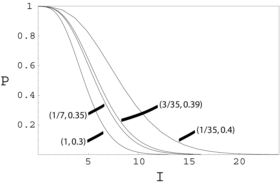
An intermittent attack can allow Eve to probe a subset of the systems very heavily, instead of probing all the systems with a weaker interaction. This peculiarity plays a non-trivial role in the case of QDC with repetition codes, where the eavesdropping of a single bit of a codeword can be sufficient to reconstruct all the encoded logical information. Here, we explicitly show the superiority of the intermittent attacks against the use of repetition codes. For the sake of simplicity, we consider only those attacks whose frequencies can be written as $\omega=t/n$, where $n$ is the length of the code and $t$ is an odd integer between $1$ and $n$.

After $N$ runs of the protocol, an intermittent attack of frequency $\omega$ (and noise $\sigma^{2}$) will affect an average of $N\omega$ systems, where $cN\omega$ are in CM and $(1-c)N\omega$ are in MM. Let us consider the MM first. For each codeword of length $n$, there is an average of $t=n\omega$ bits attacked by Eve. Over these bits, Eve adopts the criterion of majority voting in order to reconstruct the codeword. As a consequence, the probability of a logical error is equal to the probability of having at least $(t+1)/2$ bit flips, i.e.,

where $p=p(\Delta_{E})$ is the single bit-flip probability in the Alice-Eve channel, which is determined by $\Delta_{E}=1+(4\sigma^{2})^{-1}$. Then, for each MM, Eve extracts on average

bits of information. After $N$ runs of the protocol, we have an average of $(1-c)N$ instances of MM and, therefore, Eve has stolen $I=(1-c)NI_{AE}(\sigma^{2},\omega)$ bits of information. Now, let us consider the CM. For each instance of CM, Bob performs two hypothesis tests, so that an average of $2cN$ tests are done after $N$ runs of the protocol. Bob must distinguish between the two hypotheses of Eq. (13), which here means to distinguish between the two distributions $F_{\omega,0}(x)=G_{1}(x)$ (which is Gaussian) and $F_{\omega,\sigma^{2}}(x)$ with $\sigma^{2}\neq 0$ (which is non-Gaussian). Suppose that Bob knows exactly which are the instances of CM that are attacked by Eve. This assumption clearly puts a lower bound on the eavesdropping capabilities of Eve, which is however sufficient to prove the result. In this case, Bob is able to isolate the $cN\omega$ attacked instances of CM from the $cN(1-\omega)$ instances which are not attacked. On the attacked subset, Bob can now perform $2cN\omega$ tests in order to distinguish between two Gaussian distributions, i.e., $G_{1+\sigma^{2}}(x)$ and $G_{1}(x)$. Then, we have to consider the estimator of Eq. (14), but now with $M=cN\omega$. As a consequence, the survival probability of Eve after $N$ runs of the protocol is now given by $P=\Pi_{cN\omega}(\sigma^{2})$.

For every intermittent attack specified by the pair $\{\omega,\sigma^{2}\}$, we can now relate the survival probability $P$ to the number of stolen bits $I$, i.e., we can consider the function $P=P(I)$. By adopting the previous parameters for the QDC protocol, i.e., $n=35$, $\Omega=1$ and $c=1/2$, we derive the curves of Fig. 11 for different values of the pair $\{\omega,\sigma^{2}\}$. In particular, we have chosen the frequencies $\omega$ in the set $\{1,1/7,3/35,1/35\}$ and taken the corresponding optimal noises $\sigma^{2}$ which maximize Eve’s stolen information. As expected, the value of the optimal noise increases for decreasing frequency. In particular, the best performance is achieved for $\omega=1/35$ (lowest frequency) and $\sigma^{2}=0.4$ (highest noise), where Eve is able to eavesdrop $20$ bits. Notice that this value is actually a lower bound on Eve’s capabilities, i.e., Eve is able to steal at least $20$ bits. In fact, except for the case $\omega=1$ (Gaussian attack), all the curves are actually lower bounds on the actual performances of Eve. Nevertheless, this is sufficient to prove the superiority of the intermittent attacks in the eavesdropping of QDC with repetition codes. Notice that the actual performances of these non-Gaussian attacks could be much better. It is not excluded that they could completely annul the advantages brought by the use of the classical codes.

Simple variants of the previous protocols for QDC can be implemented via homodyne instead of heterodyne detection. It is sufficient that Alice encodes one single bit in the lattice by setting $U=U^{\prime}$. Then, Bob randomly switches between $\hat{q}$ and $\hat{p}$ measurements, the exact sequence being communicated to Alice at the end of the quantum communication. In such a case, Eve is forced to a delayed-choice strategy, where she has to keep all her ancillas before making the correct homodyne measurement on each of them. Similar results can be easily proven for these variants by considering that now the measurement noise is $\Delta=1/2$.

Whenever the QDC is based on heterodyne detection and implemented with a control mode probability $c=1/2$ (as in the case of the protocol of Sec. III.2), one can decide to distribute the control and message modes on all the quantum systems. This is possible by randomly choosing a quadrature for the encoding and the other for the check. Then, after Bob’s heterodyne detection, Alice declares the quadrature to be used for public comparison.

In the basic protocol of Sec. II, run-by-run and after Bob’s detection, Alice declares which mode she has used (MM or CM) and the corresponding classical information (mask amplitude $\alpha_{M}$ or signal amplitude $\bar{\alpha}$). An alternative protocol consists in delaying this declaration until the end of the quantum communication. At that point, Alice will only declare the instances in CM and the corresponding amplitudes. Such a procedure enables Alice and Bob to evaluate the noise of the channel before revealing any confidential information. From such an estimation, Alice computes the amount of information $I_{AE}$ that Eve can steal if she unmasks the message. If $I_{AE}$ is negligible (according to a pre-agreed tolerance level), then Alice unmasks all the message modes, communicating her message to Bob. Otherwise, she has to abort. Alternatively, when $I_{AE}$ is not negligible but less than $I_{AB}$, Alice and Bob can possibly use the remaining systems for distributing a secret key. Notice that such a postponed protocol takes no advantage from the use of codes. Furthermore, it can be simply implemented with $c=1/2$ and, therefore, also modified according to Sec. VI.2.

References

- [1] C. H. Bennett and G. Brassard, Proceedings of IEEE International Conference on Computers, Systems and Signal Processing (IEEE, Bangalore, India, 1984), p. 175; N. Gisin et al., Rev. Mod. Phys. 74, 145 (2002).
- [2] C. Bennett et al., Phys. Rev. Lett. 70, 1895 (1993).
- [3] T. C. Ralph, Phys. Rev. A 61, 010303(R) (2000); F. Grosshans et al., Nature 421, 238 (2003); A. M. Lance et al., Phys. Rev. Lett. 95, 180503 (2005); S. Pirandola et al., Nature Physics 4, 726 (2008).
- [4] A. Furusawa et al., Science 282, 706 (1998); Samuel L. Braunstein and H. J. Kimble, Phys. Rev. Lett. 80, 869 (1998); S. Pirandola and S. Mancini, Laser Physics 16, 1418 (2006).
- [5] S. L. Braunstein and A. K. Pati, Quantum Information Theory with Continuous Variables (Kluwer Academic, Dordrecht); S. L. Braunstein and P. van Loock, Rev. Mod. Phys. 77, 513 (2005).
- [6] S. Pirandola, S. L. Braunstein, S. Mancini, and S. Lloyd, Europhys. Lett. 84, 20013 (2008).
- [7] These classical steps are very cheap since they involve just classical computers and standard communication lines (like telephone lines).
- [8] Notice that, in a realistic experimental setting, such an intrinsic noise could include some “trusted” environmental noise which is not referable to Eve.
- [9] D. F. Walls and G. J. Milburn, Quantum Optics (Springer, Berlin, 1994).
- [10] Ideally, the two integers and are both uniformly distributed on . More realistically, we can choose two continuous values from a wide Gaussian distribution, and round them to the nearest integers.
- [11] In order to be sure that Bob has received and detected the state, Alice must require a classical communication from him.
- [12] N. J. Cerf et al., Phys. Rev. Lett. 85, 1754 (2000).
- [13] Strictly speaking, the considered machine is a and optimal UGQCM [12].
- [14] A zero-tolerance protocol does not promptly stop in realistic situations (where ) because the underlying hypothesis test is intrinsically imperfect (i.e., its probability to fail is always non-zero).
- [15] S. Pirandola, S. L. Braunstein, and S. Lloyd, Phys. Rev. Lett. 101, 200504 (2008).
- [16] A. J. Menezes, P. C. van Oorschot, and S. A. Vanstone, Handbook of Applied Cryptography (CRC Press, 1997).
- [17] M. Dušek et al., Phys. Rev. A 60, 149 (1999).