Second-Order Assortative Mixing
in Social Networks
Abstract
In a social network, the number of links of a node, or node degree, is often assumed as a proxy for the node’s importance or prominence within the network. It is known that social networks exhibit the (first-order) assortative mixing, i.e. if two nodes are connected, they tend to have similar node degrees, suggesting that people tend to mix with those of comparable prominence. In this paper, we report the second-order assortative mixing in social networks. If two nodes are connected, we measure the degree correlation between their most prominent neighbours, rather than between the two nodes themselves. We observe very strong second-order assortative mixing in social networks, often significantly stronger than the first-order assortative mixing. This suggests that if two people interact in a social network, then the importance of the most prominent person each knows is very likely to be the same. This is also true if we measure the average prominence of neighbours of the two people. This property is weaker or negative in non-social networks. We investigate a number of possible explanations for this property. However, none of them was found to provide an adequate explanation. We therefore conclude that second-order assortative mixing is a new property of social networks.
1 Background
A network or graph consists of nodes connected together via links. Networks are utilised in many disciplines. The nodes model physical elements such as people, proteins or cities, and the links between nodes represent connections between them, such as contacts, biochemical interactions, and roads. In recent years studying the structure, function and evolution of networked systems in society and nature has become a major research focus [21, 23, 2, 4, 7, 19].
The degree, , of a node is defined as the number of links the node possesses. The probability distribution of node degrees is indicative of a network’s global connectivity. For example random graphs with a Poisson degree distribution [9] have most nodes with degrees close to the average degree. In contrast, many complex networks in nature and society are scale-free graphs [1] exhibiting a power-law degree distribution, where many nodes have only a few links and a small number of nodes have very large numbers of links. However, the degree distribution alone does not provide a full description of a network’s topology. Networks with exactly the same degree distribution can possess other properties that are vastly different [15, 13, 24].
One such property, is the mixing pattern between the two end nodes of a link [18, 17], i.e. the joint probability distribution of a node with degree being connected to a node with degree . In general, biological and technological networks are disassortative mixing meaning that well-connected nodes tend to link with poorly-connected nodes, and vice versa. In contrast, social networks, such as collaborations between film actors or scientists, exhibit assortative mixing, where nodes with similar degrees tend to be connected.
To quantify this mixing property, Newman [17] proposed the assortative coefficient, , where . It is derived by considering the Pearson correlation between two sequences, where corresponding elements in the two sequences represent the degree of the nodes at either end of a link in the network. For a directed network, the degree of the starting node of a link is contained in one sequence, and the degree of the ending node is in the other sequence. The number of elements in each sequence is the number of links. For an undirected network, as all the networks studied in this paper, each undirected link is replaced by two directed links pointing at opposite directions. Thus the number of elements in a sequence is twice the number of links.
A network with assortative mixing is characterised by a possible value of ; where corresponds to a perfect assortative mixing, i.e., every link connects two nodes with the same degree. A network with disassortative mixing has a negative value of ; where corresponds to a perfect disassortative mixing, i.e., every link connects two nodes with difference degrees. When equals or close to 0, there is no degree correlation, i.e., the network is random or neutral in terms of degree mixing.
The mixing pattern has been studied as a fundamental property of networks, and the assortative coefficient has been widely used to measure this property.
2 Second-Order Mixing Pattern
We now introduce and define a related property which we refer to as the second-order mixing pattern.
2.1 Definition of and
Following Newman’s definition of the (first-order) assortative coefficient [17], we define as the second-order assortative coefficient based on the neighbours maximum degree,
| (1) |
where is the number of links in the network, and are the neighbours maximum degrees of the two nodes and connected by the link , i.e. and ; denotes the set of neighbours of node , excluding node ; and denotes the set of neighbours of node , excluding node .

Note that when calculating the first and second assortative coefficients, we actually use the excess degree [17], which is degree minus one. This is because, when considering two connected nodes, and , the neighbourhood of is defined to exclude . And likewise for the neighbourhood of . See Fig. 1 for examples.
Similarly we define as the second-order assortative coefficient based on the neighbours average degrees by replacing and in the above equation as and .
2.2 Results
| Network | Nodes | Links | |||||||
| (a) Film actor | 82,593 | 3,666,738 | 0.206 | 0.013 | 0.836 | 0.027 | 0.813 | 0.009 | 0.75 |
| (b) Scientist | 12,722 | 39,967 | 0.161 | 0.007 | 0.680 | 0.014 | 0.647 | 0.005 | 0.65 |
| (c) Musician | 198 | 2,742 | 0.020 | 0.019 | 0.543 | 0.023 | 0.307 | 0.029 | 0.62 |
| (d) Secure email | 10,680 | 24,316 | 0.238 | 0.007 | 0.653 | 0.009 | 0.680 | 0.007 | 0.27 |
| (e) General email | 1,133 | 5,451 | 0.078 | 0.014 | 0.242 | 0.014 | 0.247 | 0.014 | 0.22 |
| (f) Power grid | 4,941 | 6,594 | 0.004 | 0.014 | 0.205 | 0.015 | 0.258 | 0.016 | 0.08 |
| (g) Metabolism | 453 | 2,025 | -0.226 | 0.011 | 0.265 | 0.032 | 0.263 | 0.023 | 0.65 |
| (h) Protein | 4,626 | 14,801 | -0.137 | 0.008 | -0.046 | 0.007 | 0.033 | 0.009 | 0.09 |
| (i) Internet | 11,174 | 23,409 | -0.195 | 0.001 | -0.097 | 0.004 | 0.036 | 0.008 | 0.30 |
| (j) Random graph | 10,000 | 30,000 | 0.009 | 0.011 | 0.006 | ||||
| (k) BA graph | 10,000 | 30,000 | 0.004 | 0.008 | 0.008 |
We consider eleven networks, including five social networks, two biological networks, two technology networks, and two synthetic networks based on random connections [9] and the Barabási and Albert [1] model, respectively. Values of both the first-order and the second-order assortative coefficients, , and are provided in Table 1.
2.2.1 Statistical significance
The expected standard deviation on the value of assortative coefficient can be obtained by the jackknife method [8] as , where is the value of for the network in which the -th link is removed and . And likewise for second-order assortative coefficients and . For all cases shown in Table 1, the value of is very small (), which validates the statistical significance of the coefficients.
2.2.2 Null hypothesis test
A high correlation score between two value sequences must be tested against the null hypothesis. For each network and each coefficient in Table 1, we randomly permuted the order of degree values in one of the two degree sequences and re-computed the coefficient. This was repeated 100 times and then we calculated the mean and standard deviation. Our calculation shows that for each network and each coefficient the mean value is close to zero and the standard deviation is small. This result again confirms the statistical significance of the first and second-order assortative coefficients.
2.2.3 Social networks
Four social networks (a)-(d) show positive values of first-order assortative coefficient, and notably they show significantly higher values of second-order assortative coefficients. This indicates that in these social networks, people judge on other individual’s social status based on not only the individual’s own prominence (e.g. the number of co-starred films or co-authored publications), but more crucially, the prominence of is collaborators.
Interestingly, the Musician network exhibits very low first-order assortative mixing although it shows one of the strongest second-order assortative mixing. In other words, although musicians in this network do exhibit a strong social parity, it cannot be revealed by measuring the prominence of musicians themselves; instead we must measure the prominence of other musicians that each musician has ever performed with.
The Secure email network’s strong second-order assortative mixing is due to the security feather of this network where a person’s security credit relies on endorsement from its contacts - the more credit a contact already has the more valuable its endorsement.
2.2.4 Non-social networks
Other forms of networks do not exhibit the very strong second-order correlations exhibited by social networks.
The General email network is not considered as a typical social network, because it contains a large amount of unsolicited, one-way communications, such as notices and advertisements forwarded from departmental secretaries to all students. Not surprisingly, this network’s second assortative mixing is as weak as the Metabolism and Power grid networks.
The Internet and Protein networks, the second order assortative coefficients are either zero () or negative ().
As expected, neutral random networks generated by graph models are completely uncorrelated, i.e. .
2.3 Frequency distributions of links
Fig. 2 provides a more detailed look into the assortative mixing in the Scientist network. Fig. 2(A) shows there is a strong first-order correlation between node degrees when , and the correlation rapidly decreases with increasing degree, as expected for a scale-free network.

For the second-order assortative mixing, Fig. 2(B) shows a very strong correlation for almost all values of the neighbours maximum degree , where the link distribution along the diagonal does not decrease with the increase of . Of course the correlation in Fig. 2(B) is not perfect, and a second process appears to be uniform noise. The noise might be better modelled as Gaussian which is probably due to the summation of many nodes and the central limit theorem. If the neighbours average degree rather than the maximum is considered, we still observe a strong correlation in Fig. 2(C).
3 Seeking Possible Explanations
Here we examine whether the second-order mixing is a new topological property, i.e. whether it can be explained by other known properties of the networks.
3.1 Increased Neighbourhood
One may wonder whether the strong correlation scores associated with second-order assortative mixing could simply be due to the increased neighbourhood (from distance of one hop to two hops), as a node always has more second-order neighbours than first-order neighbours. To exclude this possibility we also examined the th-order assortative coefficients, and , which are calculated using the maximum or average degree within the neighbourhood of up to hops from each end node of a link. Of course, if the neighbourhood continues to increase, we observed that eventually the coefficients would increase and approach to one. This is to be expected since eventually, the neighbourhood encompasses the entire network.
However, we observed that for all networks under study, the values of the third-order coefficients were actually smaller than the 2nd-order coefficients. This suggest that the second-order assortative mixing cannot be explained by increased neighbourhood.
The fact that the third-order coefficients are smaller than the second-order coefficients has rich meanings. For technology networks, consider the Internet, where a network service provider only cares about the prominence of a customer (disassortative first-order mixing), it does not know and care about who else the customer has linked with (neutral second-order mixing), and care even less about those one step further away. For social networks, one tends to match its collaborator’s prominence (first-order assortative mixing) and the prominence of the collaborator’s contacts (stronger second-order assortative mixing), but it does not know or care about contacts of the collaborator’s contacts whom the collaborator does not know directly. In other words, the value of social prominence vanishes rapidly after the second-order.
3.2 High-Degree Nodes
Another possible explanation for the high values of second-order assortative coefficients considered, is that there are a few hub nodes that are extremely well connected and dominate the network structure. To test this we removed the best-connected node (together with the links attaching to it and any resulting isolated nodes) from the networks and re-computed the coefficients. We also calculate the coefficients after removing the top 5 best-connected nodes. Results show that in all cases, the coefficients change very little. For some networks, such as the Secure email, Musician and Metabolism networks, the second-order coefficients became stronger after the best-connected nodes are removed. This suggest that the second-order assortative mixing cannot be explained by the existent of high-degree nodes.
3.3 Power-Law Degree Distribution
While high degree nodes do not explain the high second order assortative mixing scores, the underlying heterogeneous power-law structure of the networks was also a possible explanation. To exclude this possibility we used the random link rewiring algorithm [15, 24] to produce surrogate networks by randomly rewiring links while preserving the exact degree distribution of the networks under study.
Fig. 2(D) illustrates the distribution of links as a function of and in a randomly rewired version of the Scientist network. The second-order assortative mixing in the original network disappears completely in the randomised case..
This result shows that the second-order mixing is not determined by a network’s degree distribution, because two networks (the original and the randomised case) with the identical degree distribution show hugely different mixing patterns, both in the first-order [15, 24] and in the second-order (see Fig. 2).
This result again demonstrates the limitation of characterising network topology by degree distribution alone, and highlights the critical importance of characterising a network’s topology using multiple properties from different aspects.
3.4 Clustering Coefficient

We also examined whether the second-order assortative mixing is a consequence of the clustering behaviour observed in many social networks, where one’s friends are also friends of each other. This is quantified by the clustering coefficient, , which is defined as , where is the degree of node and is the number of connections between the node’s neighbours [23]. The average clustering coefficient, , is the arithmetic average over all nodes in the network. Comparison of against and in Table 1 and Fig. 3 shows that high values of the second-order coefficients occur for both high and low values of clustering coefficient. There is no correlation between them.

Figure 4 reveals that the Scientist network and the Secure email network are fundamentally different in the relation between clustering coefficient and node degree, yet they have similar and . Whereas the Scientist network and the Metabolism exhibit very similar clustering coefficient properties, but their second-order coefficients are significantly different.
3.5 Common most prominent neighbour
It is interesting to consider how often the most prominent contact at each end of a link is the same person, and therefore they form a triangle. Let denote the degree difference between the most prominent neighbour of the two end nodes of a link, i.e. , and denote the number of links with . Table 2 shows the ratio of , and to the total number of links, , respectively. Note that represents the case where . Also shown is , where is the number of links for which the most prominent neighbour of the two end nodes are one and the same node and therefore forming a triangle, . Clearly the common most prominent neighbour does not provide an adequate explanation for our observations.
| Network | |||||
|---|---|---|---|---|---|
| (a) Film actor | 34.2% | 34.2% | 34.1% | 34.1% | 0.813 |
| (b) Scientist | 50.2% | 45.4% | 42.9% | 41.6% | 0.647 |
| (c) Secure email | 43.2% | 37.8% | 35.5% | 34.6% | 0.680 |
| (d) Email | 26.8% | 20.2% | 15.0% | 12.8% | 0.247 |
| (e) Musician | 56.3% | 56.0% | 55.7% | 55.7% | 0.307 |
| (f) Metabolism | 51.3% | 51.1% | 50.8% | 50.7% | 0.263 |
| (g) Protein | 10.5% | 8.0% | 6.4% | 5.7% | 0.033 |
| (h) Power grid | 68.1% | 38.3% | 19.1% | 7.8% | 0.258 |
| (i) Internet | 20.5% | 20.3% | 20.2% | 20.2% | 0.036 |
3.6 Bipartite Network
A bipartite network is a network with two non-overlapping sets of nodes and , where all links must have one end node belonging to each set. For example, actors star in films, scientist write papers, and musician play in bands. The Film actor, Scientist and Musician networks under study are constructed from bipartite networks, e.g. two actors are linked if they co-star in a film and two scientists are linked if they co-author a paper.
The Film actor, Scientist and Musician networks all exhibit strong second-order assortative mixing. It is therefore reasonable to ask whether the second-order assortative mixing can be attributed to the nature of bipartite networks? For example, all actors of one film constitute a complete subgraph, in which everyone connects with the highest-degree node in the group.
However, we found no support for this hypothesis. Firstly, the Metabolic network is also constructed from a bipartite network where the two types of nodes are metabolites and reactions. Two metabolites are linked if they participate in a reaction. The Metabolic network, however, does not show a strong second-order assortative mixing.
Secondly, the Secure email network is a non-bipartite network, where two email users are linked by direct email communications. It exhibits one of the strongest second-order assortative mixing.
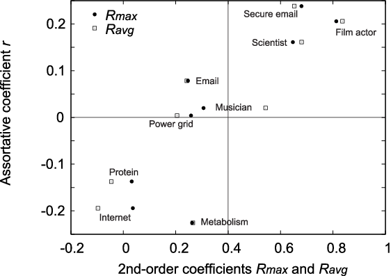
3.7 Relation Between First and Second-Order Mixing Coefficients
Figue 5 compares the assortative coefficient and the second-order coefficients and for the networks under study. They are seemingly loosely related.
However, there are exceptions. Consider the Metabolic network and the Email network, the former is strongly disassortative with , whereas the later is assortative with . Yet both networks exhibit similar values of the second-order mixing coefficients.
4 Conclusion
Our experimental results demonstrated very strong-second order assortative mixing in social networks where human are in charge of forming connections; but weaker, or even negative values for biological and technological networks where there is a lack of social preference.
We examined a larger variety of other network properties in an effort to establish whether second-order assortative mixing was induced from other network properties such as its power law distribution, cluster coefficient, and bipartite graphs. However, although some of them might be a contributing factor, none of these properties was found to provide an adequate explanation. We therefore conclude that second-order assortative mixing is a new property, which reveals a new dimension to the hierarchical structure present in social networks.
For social networks, the degree of a node is often considered a proxy for the prominence or importance of a person. First order assortative mixing has then been interpreted as indicating that if two people interact in a social network then they are likely to have similar prominence. The much stronger second-order assortative mixing suggests that there could be an even stronger social parity when measuring the prominence of a person’s contacts. Whether our most prominent contacts serve to introduce us or we simply prefer to mix with people who know similarly important people, remains an open question.
We expect that our work will provide new clues for studying the structure and evolution of social networks as well as complex networks in general.
Acknowledgments
The authors thank Ole Winther and Sune Lehmann of DTU, Denmark for discussions relating to the clustering coefficient.
References
- [1] Barabási, A. & Albert, R. (1999) Emergence of Scaling in Random Networks. Science, 286, 509.
- [2] Barabási, A. L. (2002) Linked: The New Science of Networks. Perseus Publishing.
- [3] Boguñá, M., Pastor-Satorras, R. & Vespignani, A. (2004) Cut-offs and finite size effects in scale-free networks. Eur. Phys. J. B, 38, 205–210.
- [4] Bornholdt, S. & Schuster, H. G. (2002) Handbook of Graphs and Networks - From the Genome to the Internet. Wiley-VCH, Weinheim Germany.
- [5] Colizza, V., Flammini, A., Maritan, A. & Vespignani, A. (2005) Characterization and modeling of protein–protein interaction networks. Physica A, 352, 1–27.
- [6] Dorogovtsev, S. N., Goltsev, A. V. & Mendes, J. F. F. (2002) Pseudofractal scale-free web. Physical Review E, 65, 066122.
- [7] Dorogovtsev, S. N. & Mendes, J. F. F. (2003) Evolution of Networks - From Biological Nets to the Internet and WWW. Oxford University Press, Oxford.
- [8] Efron, B. (1979) Computers and the theory of statistics thinking the unthinkable. SIAM Rev., 21, 460–480.
- [9] Erdös, P. & Rényi, A. (1959) On random graphs. Publ. Math. Debrecen, 6, 290.
- [10] Gleiser, P. & Danon, L. (2003) Community structure in jazz. Adv. Complex Syst., 6, 565–573.
- [11] Guimera, R., Danon, L., Diaz-Guilera, A., Giralt, F. & Arenas, A. (2003) Self-similar community structure in a network of human interactions. Phys. Rev. E, 68, 065103.
- [12] Jeong, H., Tombor, B., Albert, R., Oltvai, Z. N. & Barabási, A.-L. (2000) The large-scale organization of metabolic networks. Nature, 407, 651654.
- [13] Mahadevan, P., Krioukov, D., Fall, K. & Vahdat, A. (2006) Systematic Topology Analysis and Generation Using Degree Correlations. ACM SIGCOMM Comp. Comm. Revi., 36(4), 135–146.
- [14] Maslov, S. & Sneppen, K. (2002) Specificity and Stability in Topology of Protein Networks. Science, 296(5569), 910–913.
- [15] Maslov, S., Sneppenb, K. & Zaliznyaka, A. (2004) Detection of topological patterns in complex networks: correlation profile of the internet. Physica A, 333, 529–540.
- [16] Newman, M. (2001) Scientific collaboration networks. I. Network construction and fundamental results. Phys. Rev. E, 64(016131), 016131.
- [17] Newman, M. E. J. (2002) Assortative mixing in networks. Phys. Rev. Lett., 89(208701), 208701.
- [18] Pastor-Satorras, R., Vázquez, A. & Vespignani, A. (2001) Dynamical and correlation properties of the Internet. Phys. Rev. Lett., 87(258701), 258701.
- [19] Pastor-Satorras, R. & Vespignani, A. (2004) Evolution and Structure of the Internet - A Statistical Physics Approach. Cambridge University Press, Cambridge.
- [20] Ravasz, E. & Barabási, A.-L. (2003) Hierarchical organization in complex networks. Physical Review E, 67, 026112.
- [21] Wasserman, S. & Faust, K. (1994) Social Network Analysis. Cambridge University Press, Cambridge.
- [22] Watts, D. J. & Strogatz, S. H. (1998) Collective dynamics of ‘small-world’ networks. Nature, 393, 440.
- [23] Watts, J. (1999) Small Worlds: The Dynamics of Networks between Order and Randomness. Princeton Univeristy Press, New Jersey, USA.
- [24] Zhou, S. & Mondragón, R. (2007) Structural constraints in complex networks. New Journal of Physics, 9(173), 1–11.