跳到论文正文
W Papers独立论文阅读器 arXiv:0903.0649 论文正文 计算阅读时间 · 0%
引用这篇论文根据当前论文元数据生成,正式投稿前建议核对。


License: arXiv.org perpetual non-exclusive license
arXiv:0903.0649v1 [stat.ML] 03 Mar 2009

The Nonparanormal: Semiparametric Estimation of High Dimensional Undirected Graphs

Han Liu, John Lafferty, Larry Wasserman
Department of Statistics and
School of Computer Science
Carnegie Mellon University
Pittsburgh, PA 15213 USA
August 24, 2026
Abstract

Recent methods for estimating sparse undirected graphs for real-valued data in high dimensional problems rely heavily on the assumption of normality. We show how to use a semiparametric Gaussian copula—or “nonparanormal”—for high dimensional inference. Just as additive models extend linear models by replacing linear functions with a set of one-dimensional smooth functions, the nonparanormal extends the normal by transforming the variables by smooth functions. We derive a method for estimating the nonparanormal, study the method’s theoretical properties, and show that it works well in many examples.

  • Keywords:

    Graphical models, Gaussian copula, high dimensional inference, sparsity, ℓ1\ell_{1} regularization, graphical lasso, paranormal, occult

1 Introduction

The linear model is a mainstay of statistical inference that has been extended in several important ways. An extension to high dimensions was achieved by adding a sparsity constraint, leading to the lasso (Tibshirani, 1996). An extension to nonparametric models was achieved by replacing linear functions with smooth functions, leading to additive models (Hastie and Tibshirani, 1999). These two ideas were recently combined, leading to an extension called sparse additive models (SpAM) (Ravikumar et al., 2008b; Ravikumar et al., 2008a). In this paper we consider a similar nonparametric extension of undirected graphical models based on multivariate Gaussian distributions in the high dimensional setting. Specifically, we use a high dimensional Gaussian copula with nonparametric marginals, which we refer to as a nonparanormal distribution.

If XX is a pp-dimensional random vector distributed according to a multivariate Gaussian distribution with covariance matrix Σ\Sigma, the conditional independence relations between the random variables X1,X2,…,XpX_{1},X_{2},\ldots,X_{p} are encoded in a graph formed from the precision matrix Ω=Σ−1\Omega=\Sigma^{-1}. Specifically, missing edges in the graph correspond to zeroes of Ω\Omega. To estimate the graph from a sample of size nn, it is only necessary to estimate Σ\Sigma, which is easy if nn is much larger than pp. However, when pp is larger than nn, the problem is more challenging. Recent work has focused on the problem of estimating the graph in this high dimensional setting, which becomes feasible if GG is sparse. Yuan and Lin (2007) and Banerjee et al. (2008) propose an estimator based on regularized maximum likelihood using an ℓ1\ell_{1} constraint on the entries of Ω\Omega, and Friedman et al. (2007) develop an efficient algorithm for computing the estimator using a graphical version of the lasso. The resulting estimation procedure has excellent theoretical properties, as shown recently by Rothman et al. (2008) and Ravikumar et al. (2009).

While Gaussian graphical models can be useful, a reliance on exact normality is limiting. Our goal in this paper is to weaken this assumption. Our approach parallels the ideas behind sparse additive models for regression (Ravikumar et al., 2008b; Ravikumar et al., 2008a). Specifically, we replace the Gaussian with a semiparametric Gaussian copula. This means that we replace the random variable X=(X1,…,Xp)X=(X_{1},\ldots,X_{p}) by the transformed random variable f⁡(X)=(f1​(X1),…,fp​(Xp))f(X)=\left(f_{1}(X_{1}),\ldots,f_{p}(X_{p})\right), and assume that f⁡(X)f(X) is multivariate Gaussian. This semiparametric copula results in a nonparametric extension of the normal that we call the nonparanormal distribution. The nonparanormal depends on the functions {fj}\{f_{j}\}, and a mean μ\mu and covariance matrix Σ\Sigma, all of which are to be estimated from data. While the resulting family of distributions is much richer than the standard parametric normal (the paranormal), the independence relations among the variables are still encoded in the precision matrix Ω=Σ−1\Omega=\Sigma^{-1}. We propose a nonparametric estimator for the functions {fj}\{f_{j}\}, and show how the graphical lasso can be used to estimate the graph in the high dimensional setting. The relationship between linear regression models, Gaussian graphical models, and their extensions to nonparametric and high dimensional models is summarized in Figure 1.

Most theoretical results on semiparametric copulas focus on low or at least finite dimensional models (Tsukahara, 2005). Models with increasing dimension require a more delicate analysis; in particular, simply plugging in the usual empirical distribution of the marginals does not lead to accurate inference. Instead we use a truncated empirical distribution. We give a theoretical analysis of this estimator, proving consistency results with respect to risk, model selection, and estimation of Ω\Omega in the Frobenius norm.

In the following section we review the basic notion of the graph corresponding to a multivariate Gaussian, and formulate different criteria for evaluating estimators of the covariance or inverse covariance. In Section 3 we present the nonparanormal, and in Section 4 we discuss estimation of the model. We present a theoretical analysis of the estimation method in Section 5, with the detailed proofs collected in an appendix. In Section 6 we present experiments with both simulated data and gene microarray data, where the problem is to construct the isoprenoid biosynthetic pathway.

Assumptions Dimension Regression Graphical Models
parametric low linear model multivariate normal
high lasso graphical lasso
nonparametric low additive model nonparanormal
high sparse additive model ℓ1\ell_{1}-regularized nonparanormal
Figure 1: Comparison of regression and graphical models. The nonparanormal extends additive models to the graphical model setting. Regularizing the inverse covariance leads to an extension to high dimensions, which parallels sparse additive models for regression.

2 Estimating Undirected Graphs

Let X=(X1,…,Xp)X=(X_{1},\ldots,X_{p}) denote a random vector with distribution P=N⁡(μ,Σ)P=N(\mu,\Sigma). The undirected graph G=(V,E)G=(V,E) corresponding to PP consists of a vertex set VV and an edge set EE. The set VV has pp elements, one for each component of XX. The edge set EE consists of ordered pairs (i,j)(i,j) where (i,j)∈E(i,j)\in E if there is a edge between XiX_{i} and XjX_{j}. The edge between (i,j)(i,j) is excluded from EE if and only if XiX_{i} is independent of XjX_{j} given the other variables O\{i,j}≡(Xs: 1≤s≤p,s≠i,j)O_{\backslash\{i,j\}}\equiv(X_{s}:\ 1\leq s\leq p,\ \ s\neq i,j), written

Xi∐Xj|O\{i,j}.X_{i}\amalg X_{j}\Bigm|O_{\backslash\{i,j\}}. (1)

It is well-known that, for multivariate Gaussian distributions, (1) holds if and only if Ωi​j=0\Omega_{ij}=0 where Ω=Σ−1\Omega=\Sigma^{-1}.

Let X(1),X(2),…,X(n)X^{(1)},X^{(2)},\ldots,X^{(n)} be a random sample from PP, where X(i)∈ℝpX^{(i)}\in{\mathbb{R}}^{p}. If nn is much larger than pp, then we can estimate Σ\Sigma using maximum likelihood, leading to the estimate Ω^=S−1\widehat{\Omega}=S^{-1}, where

S=1n​∑i=1n(X(i)−X¯)​(X(i)−X¯)TS=\frac{1}{n}\sum_{i=1}^{n}\left(X^{(i)}-\overline{X}\right)\left(X^{(i)}-\overline{X}\right)^{T}

is the sample covariance, with X¯\overline{X} the sample mean. The zeroes of Ω\Omega can then be estimated by applying hypothesis testing to Ω^\widehat{\Omega} (Drton and Perlman, 2007; Drton and Perlman, 2008).

When p>np>n, maximum likelihood is no longer useful; in particular, the estimate Σ^\widehat{\Sigma} is not positive definite, having rank no greater than nn. Inspired by the success of the lasso for linear models, several authors have suggested estimating Σ\Sigma by minimizing

−ℓ⁡(μ,Ω)+λ​∑j≠k|Ωj​k|-\ell(\mu,\Omega)+\lambda\sum_{j\neq k}|\Omega_{jk}| (2)

where

ℓ⁡(μ,Ω)=12​(log⁡|Ω|−tr​(Ω​S)−p​log⁡(2​π))\ell(\mu,\Omega)=\frac{1}{2}\left(\log|\Omega|-\text{tr}(\Omega S)-p\log(2\pi)\right) (3)

is the average log-likelihood and SS is the sample covariance matrix. The estimator Ω^\widehat{\Omega} can be computed efficiently using the glasso algorithm (Friedman et al., 2007), which is a block coordinate descent algorithm that uses the standard lasso to estimate a single row and column of Ω\Omega in each iteration. Under appropriate sparsity conditions, the resulting estimator Ω^\widehat{\Omega} has been shown to have good theoretical properties (Rothman et al., 2008; Ravikumar et al., 2009).

There are several different ways to judge the quality of an estimator Σ^\widehat{\Sigma} of the covariance or inverse covariance Ω^\widehat{\Omega}. We discuss three in this paper, persistency, norm consistency, and sparsistency. Persistency means consistency in risk, when the model is not assumed to be correct. Suppose the true distribution is PP has mean μ0\mu_{0}, and that we use a multivariate normal p⁡(x,μ0,Σ)p(x;\mu_{0},\Sigma) for prediction. We do not assume that PP is normal. We observe a new vector X∼PX\sim P and define the prediction risk to be

R(Σ)=−𝔼logp(X;μ0,Σ)=−∫logp(x;μ0,Σ)dP(x).R(\Sigma)=-\mathbb{E}\log p(X;\mu_{0},\Sigma)=-\int\log p(x;\mu_{0},\Sigma)\,dP(x).

It follows that

R⁡(Σ)=12​(tr​(Σ−1​Σ0)+log⁡|Σ|−p​log⁡(2​π))R(\Sigma)=\frac{1}{2}\left(\text{tr}(\Sigma^{-1}\Sigma_{0})+\log|\Sigma|-p\log(2\pi)\right)

where Σ0\Sigma_{0} is the covariance of XX under PP. If 𝒮{\cal S} is a set of covariance matrices, the oracle is defined to be the covariance matrix Σ∗\Sigma_{*} that minimizes R⁡(Σ)R(\Sigma) over 𝒮{\cal S}:

Σ∗=arg minΣ∈𝒮⁡R⁡(Σ).\Sigma_{*}={\mathop{\text{arg\,min}}}_{\Sigma\in{\cal S}}R(\Sigma).

Thus p⁡(x,μ0,Σ∗)p(x;\mu_{0},\Sigma_{*}) is the best predictor of a new observation among all distributions in {p⁡(x,μ0,Σ):Σ∈𝒮}\{p(x;\mu_{0},\Sigma):\ \Sigma\in{\cal S}\}. In particular, if 𝒮{\cal S} consists of covariance matrices with sparse graphs, then p⁡(x,μ0,Σ∗)p(x;\mu_{0},\Sigma_{*}) is, in some sense, the best sparse predictor. An estimator Σ^n\widehat{\Sigma}_{n} is persistent if

R⁡(Σ^n)−R⁡(Σ∗)→P0R(\widehat{\Sigma}_{n})-R(\Sigma_{*})\stackrel{{\scriptstyle P}}{{\rightarrow}}0

as the sample size nn increases to infinity. Thus, a persistent estimator approximates the best estimator over the class 𝒮{\cal S}, but we do not assume that the true distribution has a covariance matrix in 𝒮{\cal S}, or even that it is Gaussian. Moreover, we allow the dimension p=pnp=p_{n} to increase with nn. On the other hand, norm consistency and sparsistency require that the true distribution is Gaussian. In this case, let Σ0\Sigma_{0} denote the true covariance matrix. An estimator is norm consistent if

‖Σ^n−Σ‖→P0\|\widehat{\Sigma}_{n}-\Sigma\|\stackrel{{\scriptstyle P}}{{\to}}0

where ∥⋅∥\|\cdot\| is a norm. If E⁡(Ω)E(\Omega) denotes the edge set corresponding to Ω\Omega. An estimator is sparsistent if

ℙ⁡(E⁡(Ω)≠E⁡(Ω^n))→0.\mathbb{P}\Bigl(E(\Omega)\neq E(\widehat{\Omega}_{n})\Bigr)\rightarrow 0.

Thus, a sparsistent estimator identifies the correct graph consistently. We summarize known results on these properties for the multivariate normal in Section 5, before presenting our theoretical analysis of the nonparanormal.

3 The Nonparanormal

We say that a random vector X=(X1,…,Xp)TX=(X_{1},\ldots,X_{p})^{T} has a nonparanormal distribution if there exist functions {fj}j=1p\{f_{j}\}_{j=1}^{p} such that Z≡f⁡(X)∼N⁡(μ,Σ)Z\equiv f(X)\sim N(\mu,\Sigma), where f⁡(X)=(f1​(X1),…,fp​(Xp))f(X)=(f_{1}(X_{1}),\ldots,f_{p}(X_{p})). We then write

X∼NPN ⁡(μ,Σ,f).X\sim\mathop{\textit{NPN\,}}(\mu,\Sigma,f).

When the fjf_{j}’s are monotone and differentiable, the joint probability density function of XX is given by

pX​(x)=1(2​π)p/2​|Σ|1/2​exp⁡{−12​(f⁡(x)−μ)T​Σ−1​(f⁡(x)−μ)}​∏j=1p|fj′​(xj)|.p_{X}(x)=\frac{1}{(2\pi)^{p/2}|\Sigma|^{1/2}}\exp\left\{-\frac{1}{2}\left(f(x)-\mu\right)^{T}{\Sigma}^{-1}\left(f(x)-\mu\right)\right\}\prod_{j=1}^{p}|f^{\prime}_{j}(x_{j})|. (4)
Lemma 3.1

.  The nonparanormal distribution NPN ⁡(μ,Σ,f)\mathop{\textit{NPN\,}}(\mu,\Sigma,f) is a Gaussian copula when the fjf_{j}’s are monotone and differentiable.

Proof. By Sklar’s theorem (Sklar, 1959), any joint distribution can be written as

F⁡(x1,…,xp)=C⁡{F1​(x1),…,Fp​(xp)}F(x_{1},\ldots,x_{p})=C\{F_{1}(x_{1}),\ldots,F_{p}(x_{p})\}

where the function CC is called a copula. For the nonparanormal we have

F⁡(x1,…,xp)=Φμ,Σ​(Φ−1​(F1​(x1)),…,Φ−1​(Fp​(xp)))F(x_{1},\ldots,x_{p})=\Phi_{\mu,\Sigma}(\Phi^{-1}(F_{1}(x_{1})),\ldots,\Phi^{-1}(F_{p}(x_{p})))

where Φμ,Σ\Phi_{\mu,\Sigma} is the multivariate Gaussian cdf and Φ\Phi is the univariate standard Gaussian cdf. Thus, the corresponding copula is

C⁡(u1,…,up)=Φμ,Σ​(Φ−1​(u1),…,Φ−1​(up)).C(u_{1},\ldots,u_{p})=\Phi_{\mu,\Sigma}(\Phi^{-1}(u_{1}),\ldots,\Phi^{-1}(u_{p})).

This is exactly a Gaussian copula with parameters μ\mu and Σ\Sigma. If each fjf_{j} is differentiable then the density of XX has the same form as (4).  □\;\;\scriptstyle\Box

Note that the density in (4) is not identifiable; to make the family identifiable we demand that fjf_{j} preserve means and variances:

μj=𝔼⁡(Zj)=𝔼⁡(Xj)​and​σj2≡Σj​j=Var⁡(Zj)=Var⁡(Xj).\mu_{j}=\mathbb{E}(Z_{j})=\mathbb{E}(X_{j})~~\mathrm{and}~~\sigma^{2}_{j}\equiv\Sigma_{jj}=\mathrm{Var}\left(Z_{j}\right)=\mathrm{Var}\left(X_{j}\right). (5)

Note that these conditions only depend on diag⁡(Σ)\mathrm{diag}(\Sigma) but not the full covariance matrix.

Let Fj​(x)F_{j}(x) denote the marginal distribution function of XjX_{j}. Then

Fj​(x)=ℙ⁡(Xj≤x)=ℙ⁡(Zj≤fj​(x))=Φ⁡(fj​(x)−μjσj)F_{j}(x)=\mathbb{P}\left(X_{j}\leq x\right)=\mathbb{P}\left(Z_{j}\leq f_{j}(x)\right)=\Phi\left(\frac{f_{j}(x)-\mu_{j}}{\sigma_{j}}\right)

which implies that

fj​(x)=μj+σj​Φ−1​(Fj​(x)).f_{j}(x)=\mu_{j}+\sigma_{j}\Phi^{-1}\left(F_{j}(x)\right).

The following basic fact says that the independence graph of the nonparanormal is encoded in Ω=Σ−1\Omega=\Sigma^{-1}, as for the parametric normal.

Lemma 3.2

.  If X∼NPN ⁡(μ,Σ,f)X\sim\mathop{\textit{NPN\,}}(\mu,\Sigma,f) is nonparanormal and each fjf_{j} is differentiable, then Xi∐Xj|O\{i,j}X_{i}\amalg X_{j}{\,|\,}O_{\backslash\{i,j\}} if and only if Ωi​j=0\Omega_{ij}=0, where Ω=Σ−1\Omega=\Sigma^{-1}.

Proof. From the form of the density (4), it follows that the density factors with respect to the graph of Ω\Omega, and therefore obeys the global Markov property of the graph.  □\;\;\scriptstyle\Box

Refer to caption Refer to caption Refer to caption
Figure 2: Densities of three 2-dimensional nonparanormals. The component functions have the form fj​(x)=sign​(x)​|x|αjf_{j}(x)=\text{sign}(x)|x|^{\alpha_{j}}. Left: α1=0.9\alpha_{1}=0.9, α2=0.8\alpha_{2}=0.8; center: α1=1.2\alpha_{1}=1.2, α2=0.8\alpha_{2}=0.8; right α1=2\alpha_{1}=2, α2=3\alpha_{2}=3. In each case μ=(0,0)\mu=(0,0) and Σ=(1 .5.5 1)\Sigma=\binom{1\ .5}{.5\ 1}.

Next we show that the above is true for any choice of identification restrictions.

Lemma 3.3

.  Define

hj​(x)=Φ−1​(Fj​(x))h_{j}(x)=\Phi^{-1}(F_{j}(x)) (6)

and let Λ\Lambda be the covariance matrix of h⁡(X)h(X). Then Xj∐Xk|O\{j,k}X_{j}\amalg X_{k}{\,|\,}O_{\backslash\{j,k\}} if and only if Λj​k−1=0\Lambda_{jk}^{-1}=0.

Proof. We can rewrite the covariance matrix as

Σj​k=Cov⁡(Zj,Zk)=σj​σk​Cov​(hj​(Xj),hk​(Xk)).\Sigma_{jk}={\rm Cov}(Z_{j},Z_{k})=\sigma_{j}\sigma_{k}{\rm Cov}(h_{j}(X_{j}),h_{k}(X_{k})).

Hence Σ=D​Λ​D\Sigma=D\Lambda D and

Σ−1=D−1​Λ−1​D−1.\Sigma^{-1}=D^{-1}\Lambda^{-1}D^{-1}.

where DD is the diagonal matrix with diag​(D)=σ\text{diag}(D)=\sigma. The zero pattern of Λ−1\Lambda^{-1} is therefore identical to the zero pattern of Σ−1\Sigma^{-1}.  □\;\;\scriptstyle\Box

Thus, it is not necessary to estimate μ\mu or σ\sigma to estimate the graph.

Figure 2 shows three examples of 2-dimensional nonparanormal densities. In each case, the component functions fj​(x)f_{j}(x) take the form

fj​(x)=aj​sign​(x)​|x|αj+bjf_{j}(x)=a_{j}\text{sign}(x)|x|^{\alpha_{j}}+b_{j}

where the constants aja_{j} and bjb_{j} are set to enforce the identifiability constraints (5). The covariance in each case is Σ=(1 .5.5 1)\Sigma=\binom{1\ .5}{.5\ 1} and the mean is μ=(0,0)\mu=(0,0). The exponent αj\alpha_{j} determines the nonlinearity. It can be seen how the concavity of the density changes with the exponent α\alpha, and that α>1\alpha>1 can result in multiple modes.

The assumption that f⁡(X)=(f1​(X1),…,fp​(Xp)CLOSEf(X)=(f_{1}(X_{1}),\ldots,f_{p}(X_{p}) is normal leads to a semiparametric model where only one dimensional functions need to be estimated. But the monotonicity of the functions fjf_{j}, which map onto ℝ{\mathbb{R}}, enables computational tractability of the nonparanormal. For more general functions ff, the normalizing constant for the density

pX​(x)∝exp⁡{−12​(f⁡(x)−μ)T​Σ−1​(f⁡(x)−μ)}p_{X}(x)\propto\exp\left\{-\frac{1}{2}\left(f(x)-\mu\right)^{T}{\Sigma}^{-1}\left(f(x)-\mu\right)\right\}

cannot be computed in closed form.

4 Estimation Method

Let X(1),…,X(n)X^{(1)},\ldots,X^{(n)} be a sample of size nn where X(i)=(X1(i),…,Xp(i))T∈ℝpX^{(i)}=(X^{(i)}_{1},\ldots,X^{(i)}_{p})^{T}\in\mathbb{R}^{p}. In light of (6) we define

h^j​(x)=Φ−1​(F~j​(x))\widehat{h}_{j}(x)=\Phi^{-1}(\widetilde{F}_{j}(x))

where F~j\widetilde{F}_{j} is an estimator of FjF_{j}. A natural candidate for F~j\widetilde{F}_{j} is the marginal empirical distribution function

F^j(t)≡1n∑i=1n𝟏{X(i)j≤t}.\widehat{F}_{j}(t)\equiv\frac{1}{n}\sum_{i=1}^{n}\mathbf{1}_{\left\{X^{(i)}_{j}\leq t\right\}}.

Now, let θ\theta denote the parameters of the copula. Tsukahara (2005) suggests taking θ^\widehat{\theta} to be the solution of

∑i=1nϕ⁡(F~1​(X1(i)),…,F~p​(Xp(i)),θ)=0\sum_{i=1}^{n}\phi\left(\widetilde{F}_{1}(X_{1}^{(i)}),\ldots,\widetilde{F}_{p}(X_{p}^{(i)}),\theta\right)=0

where ϕ\phi is an estimating equation and F~j​(t)=n​F^j​(t)/(n+1)\widetilde{F}_{j}(t)=n\widehat{F}_{j}(t)/(n+1). In our case, θ\theta corresponds to the covariance matrix. The resulting estimator θ^\widehat{\theta}, called a rank approximate ZZ-estimator, has excellent theoretical properties. However, we are interested in the high dimensional scenario where the dimension pp is allowed to increase with nn; the variance of F^j​(t)\widehat{F}_{j}(t) is too large in this case. Instead, we use the following truncated or Winsorized11 1 After Charles P. Winsor, whom John Tukey credited with converting him from topology to statistics (Mallows, 1990). estimator:

F~j​(x)={δnif F^j​(x)<δnF^j​(x)if δn≤F^j​(x)≤1−δn(1−δn)if F^j​(x)>1−δn,\widetilde{F}_{j}(x)=\begin{cases}\delta_{n}&\text{if $\widehat{F}_{j}(x)<\delta_{n}$}\\ \widehat{F}_{j}(x)&\text{if $\delta_{n}\leq\widehat{F}_{j}(x)\leq 1-\delta_{n}$}\\ (1-\delta_{n})&\text{if $\widehat{F}_{j}(x)>1-\delta_{n}$},\end{cases} (7)

where δn\delta_{n} is a truncation parameter. Clearly, there is a bias-variance tradeoff in choosing δn\delta_{n}. In what follows we use

δn≡14​n1/4​π​log⁡n.\delta_{n}\equiv\frac{1}{4n^{1/4}\sqrt{\pi\log n}}. (8)

This provides the right balance so that we can achieve the desired rate of convergence in our estimate of Ω\Omega and the associated undirected graph GG.

Given this estimate of the distribution of variable XjX_{j}, we then estimate the transformation function fjf_{j} by

f~j​(x)≡μ^j+σ^j​h~j​(x)\displaystyle\widetilde{f}_{j}(x)\equiv\widehat{\mu}_{j}+\widehat{\sigma}_{j}\widetilde{h}_{j}(x) (9)

where

h~j​(x)=Φ−1​(F~j​(x))\widetilde{h}_{j}(x)=\Phi^{-1}\left(\widetilde{F}_{j}(x)\right)

and μ^j\widehat{\mu}_{j} and σ^j\widehat{\sigma}_{j} are the sample mean and the standard deviation:

μ^j≡1n​∑i=1nXj(i)​and​σ^j=1n​∑i=1n(Xj(i)−μ^j)2.\widehat{\mu}_{j}\equiv\frac{1}{n}\sum_{i=1}^{n}X^{(i)}_{j}~~\mathrm{and}~~\widehat{\sigma}_{j}=\sqrt{\frac{1}{n}\sum_{i=1}^{n}\left(X^{(i)}_{j}-\widehat{\mu}_{j}\right)^{2}}.

Now, let Sn​(f~)S_{n}(\widetilde{f}) be the sample covariance matrix of f~​(X(1)),…,f~​(X(n))\widetilde{f}(X^{(1)}),\ldots,\widetilde{f}(X^{(n)}); that is,

Sn​(f~)\displaystyle S_{n}(\widetilde{f}) ≡\displaystyle\equiv 1n​∑i=1n(f~​(X(i))−μn​(f~))​(f~​(X(i))−μn​(f~))T\displaystyle\frac{1}{n}\sum_{i=1}^{n}\left(\widetilde{f}(X^{(i)})-\mu_{n}(\widetilde{f})\right)\left(\widetilde{f}(X^{(i)})-\mu_{n}(\widetilde{f})\right)^{T} (10)
μn​(f~)\displaystyle\mu_{n}(\widetilde{f}) ≡\displaystyle\equiv 1n​∑i=1nf~​(X(i)).\displaystyle\frac{1}{n}\sum_{i=1}^{n}\widetilde{f}(X^{(i)}).

We then estimate Ω\Omega using Sn​(f~)S_{n}(\widetilde{f}). For instance, the maximum likelihood estimator is Ω^n=Sn​(f~)−1\widehat{\Omega}_{n}=S_{n}(\widetilde{f})^{-1}. The ℓ1\ell_{1}-regularized estimator is

Ω^n=arg minΩ⁡{tr​(Ω​Sn​(f~))−log⁡|Ω|+λ​‖Ω‖1}\widehat{\Omega}_{n}=\mathop{\text{arg\,min}}_{\Omega}\left\{\text{tr}\left(\Omega S_{n}(\widetilde{f})\right)-\log|\Omega|+\lambda\|\Omega\|_{1}\right\} (11)

where λ\lambda is a regularization parameter, and ‖Ω‖1=∑j≠k|Ωj​k|\|\Omega\|_{1}=\sum_{j\neq k}|\Omega_{jk}|. The estimated graph is then E^n={(j,k):Ω^j​k≠0}\widehat{E}_{n}=\{(j,k):\ \widehat{\Omega}_{jk}\neq 0\}. In the following section we analyze the theoretical properties of this ℓ1\ell_{1}-regularized estimator.

5 Theoretical Results

In this section we present our theoretical results on risk consistency, model selection consistency, and norm consistency of the covariance Σ\Sigma and inverse covariance Ω\Omega. From Lemma 3.3, the estimate of the graph does not depend on σj,j∈{1,…,p}\sigma_{j},\;j\in\{1,\ldots,p\} and μ\mu, so we assume that σj=1\sigma_{j}=1 and μ=0\mu=0. Our key technical result is an analysis of covariance of the Winsorized estimator defined in (7), (9), and (10). In particular, we show that under appropriate conditions,

maxj,k⁡|Sn​(f~)j​k−Sn​(f)j​k|=OP​(log⁡p​log2​nn1/2)\max_{j,k}\left|S_{n}(\widetilde{f})_{jk}-S_{n}(f)_{jk}\right|=O_{P}\left(\sqrt{\frac{\log p\log^{2}n}{n^{1/2}}}\right)

where Sn​(f~)j​kS_{n}(\widetilde{f})_{jk} denotes the (j,k)(j,k) entry of the matrix. This result allows us to leverage the recent analysis of Rothman et al. (2008) and Ravikumar et al. (2009) in the Gaussian case to obtain consistency results for the nonparanormal. More precisely, our main theorem is the following.

Theorem 5.1

.  Suppose that p=nξp=n^{\xi} and let f~\widetilde{f} be the Winsorized estimator defined in (9) with δn=14​n1/4​π​log⁡n\delta_{n}=\displaystyle\frac{1}{4n^{1/4}\sqrt{\pi\log n}}. Define

C⁡(M,ξ)≡48π​ξ​(2​M−1)​(M+2)\displaystyle C(M,\xi)\equiv\frac{48}{\sqrt{\pi\xi}}\left(\sqrt{2M}-1\right)(M+2)

for M,ξ>0M,\xi>0. Then for any ϵ≥C⁡(M,ξ)​log⁡p​log2​nn1/2\displaystyle\epsilon\geq C(M,\xi)\sqrt{\frac{\log p\log^{2}n}{n^{1/2}}} and sufficiently large nn, we have

ℙ⁡(maxj​k⁡|Sn​(f~)j​k−Sn​(f)j​k|>ϵ)≤c1​p(n​ϵ2)2​ξ+c2​pnM​ξ−1+c3​exp⁡(−c4​n1/2​ϵ2log⁡p​log2​n),\displaystyle\mathbb{P}\left(\max_{jk}\left|S_{n}(\widetilde{f})_{jk}-S_{n}(f)_{jk}\right|>\epsilon\right)\leq\frac{c_{1}p}{(n\epsilon^{2})^{2\xi}}+\frac{c_{2}p}{n^{M\xi-1}}+c_{3}\exp\left(-\frac{c_{4}n^{1/2}\epsilon^{2}}{\log p\log^{2}n}\right),

where c1,c2,c3,c4c_{1},c_{2},c_{3},c_{4} are positive constants.

The proof of the above theorem is given in Section 7. The following corollary is immediate, which specifies the scaling of the dimension in terms of sample size.

Corollary 5.2

.  Let M>1+1ξM>\displaystyle 1+\frac{1}{\xi}. Then

ℙ⁡(maxj​k⁡|Sn​(f~)j​k−Sn​(f)j​k|>C⁡(M,ξ)​log⁡p​log2​nn1/2)=o⁡(1)+c3​exp⁡(−c4​C2​(M,ξ)).\displaystyle\mathbb{P}\left(\max_{jk}\left|S_{n}(\widetilde{f})_{jk}-S_{n}(f)_{jk}\right|>C(M,\xi)\sqrt{\frac{\log p\log^{2}n}{n^{1/2}}}\right)=o(1)+c_{3}\exp\left(-c_{4}C^{2}(M,\xi)\right).

Hence,

maxj,k⁡|Sn​(f~)j​k−Sn​(f)j​k|=OP​(log⁡p​log2​nn1/2).\displaystyle\max_{j,k}\left|S_{n}(\widetilde{f})_{jk}-S_{n}(f)_{jk}\right|=O_{P}\left(\sqrt{\frac{\log p\log^{2}n}{n^{1/2}}}\right). (12)

The following corollary yields estimation consistency in both the Frobenius norm and the ℓ2\ell_{2}-operator norm. The proof follows the same arguments as the proof of Theorem 1 and Theorem 2 from Rothman et al. (2008), replacing their Lemma 1 with our Theorem 5.1.

For a matrix A=(ai​j)A=(a_{ij}), the Frobenius norm ∥⋅∥F\|\cdot\|_{F} is defined as ‖A‖F≡∑i,jai​j2\|A\|_{\rm F}\equiv\sqrt{\sum_{i,j}a^{2}_{ij}}. The ℓ2\ell_{2}-operator norm ∥⋅∥2\|\cdot\|_{2} is defined as the magnitude of the largest eigenvalue of the matrix, ‖A‖2≡max‖x‖2=1⁡‖A​x‖2\|A\|_{2}\equiv\max_{\|x\|_{2}=1}\|Ax\|_{2}. In the following, we write an≍bna_{n}\asymp b_{n} if there are positive constants cc and CC independent of nn such that c≤an/bn≤Cc\leq{a_{n}}/{b_{n}}\leq C.

Corollary 5.3

.  Suppose that the data are generated as X(i)∼NPN ⁡(μ0,Σ0,f0)X^{(i)}\sim\mathop{\textit{NPN\,}}(\mu_{0},\Sigma_{0},f_{0}), and let Ω0=Σ0−1\Omega_{0}=\Sigma_{0}^{-1}. If the regularization parameter λn\lambda_{n} is chosen as

λn≍log⁡p​log2​nn1/2\displaystyle\lambda_{n}\asymp\sqrt{\frac{\log p\log^{2}n}{n^{1/2}}}

then the nonparanormal estimator Ω^n\widehat{\Omega}_{n} of (11) satisfies

‖Ω^n−Ω0‖F=OP​((s+p)​log⁡p​log2​nn1/2)\displaystyle\|\widehat{\Omega}_{n}-\Omega_{0}\|_{\rm F}=O_{P}\left(\sqrt{\frac{(s+p)\log p\log^{2}n}{n^{1/2}}}\right)

and

‖Ω^n−Ω0‖2=OP​(s​log⁡p​log2​nn1/2),\displaystyle\|\widehat{\Omega}_{n}-\Omega_{0}\|_{2}=O_{P}\left(\sqrt{\frac{s\log p\log^{2}n}{n^{1/2}}}\right),

where

s≡Card({(i,j)∈{1,…,p}×{1,…,p}|Ω0(i,j)≠0,i≠j})\displaystyle s\equiv\mathrm{Card}\left(\left\{(i,j)\in\{1,\ldots,p\}\times\{1,\ldots,p\}{\,|\,}{{\Omega_{0}}(i,j)}\neq 0,~i\neq j\right\}\right)

is the number of nonzero off-diagonal elements of the true precision matrix.

To prove the model selection consistency result, we need further assumptions. We follow Ravikumar (2009) and let the p2×p2p^{2}\times p^{2} Fisher information matrix of Σ0\Sigma_{0} be Γ≡Σ0⊗Σ0\Gamma\equiv\Sigma_{0}\otimes\Sigma_{0} where ⊗\otimes is the Kronecker matrix product, and define the support set SS of Ω0=Σ0−1\Omega_{0}=\Sigma_{0}^{-1} as

S≡{(i,j)∈{1,…,p}×{1,…,p}|Ω0​(i,j)≠0}.\displaystyle S\equiv\left\{(i,j)\in\{1,\ldots,p\}\times\{1,\ldots,p\}{\,|\,}\Omega_{0}(i,j)\neq 0\right\}.

We use ScS^{c} to denote the complement of SS in the set {1,…,p}×{1,…,p}\{1,\ldots,p\}\times\{1,\ldots,p\}, and for any two subsets TT and T′T^{\prime} of {1,…,p}×{1,…,p}\{1,\ldots,p\}\times\{1,\ldots,p\}, we use ΓT​T′\Gamma_{TT^{\prime}} to denote the sub-matrix with rows and columns of Γ\Gamma indexed by TT and T′T^{\prime} respectively.

Assumption 5.4

.  There exists some α∈(0,1]\alpha\in(0,1], such that ‖ΓSc​S​(ΓS​S)−1‖∞≤1−α.\left\|\Gamma_{S^{c}S}(\Gamma_{SS})^{-1}\right\|_{\infty}\leq 1-\alpha.

As in Ravikumar et al. (2009), we define two quantities KΣ0≡‖Σ0‖∞K_{\Sigma_{0}}\equiv\|\Sigma_{0}\|_{\infty} and KΓ≡‖(ΓS​S)−1‖∞K_{\Gamma}\equiv\|(\Gamma_{SS})^{-1}\|_{\infty}. Further, we define the maximum row degree as

d≡maxi=1,…,pCard({j∈1,…,p|Ω0(i,j)≠0}).\displaystyle d\equiv\max_{i=1,\ldots,p}\mathrm{Card}\left(\{j\in{1,\ldots,p}{\,|\,}\Omega_{0}(i,j)\neq 0\}\right).
Assumption 5.5

.  The quantities KΣ0K_{\Sigma^{0}} and KΓK_{\Gamma} are bounded, and there are positive constants C1C_{1} and C2C_{2} such that

min(j,k)∈S⁡|Ω0​(j,k)|≥C1​log⁡nn​and​n≥C2​d2​log⁡p\displaystyle\min_{(j,k)\in S}\left|\Omega_{0}(j,k)\right|\geq C_{1}\sqrt{\frac{\log n}{n}}~~\mathrm{and}~~n\geq C_{2}d^{2}\log p

for large enough nn.

The proof of the following uses our Theorem 5.1 in place of equation (12) in the analysis of Ravikumar et al. (2009),

Corollary 5.6

.  Suppose the regularization parameter is chosen as

λn≍log⁡p​log2​nn1/2.\displaystyle\lambda_{n}\asymp\sqrt{\frac{\log p\log^{2}n}{n^{1/2}}}.

Then the nonparanormal estimator Ω^n\widehat{\Omega}_{n} satisfies

ℙ⁡(𝒢⁡(Ω^n,Ω0))≥1−o⁡(1)\displaystyle\mathbb{P}\left({\mathcal{G}}\left(\widehat{\Omega}_{n},\Omega_{0}\right)\right)\geq 1-o(1)

where 𝒢⁡(Ω^n,Ω0){\mathcal{G}}(\widehat{\Omega}_{n},\Omega_{0}) is the event

{sign⁡(Ω^n​(j,k))=sign⁡(Ω0−1​(j,k)),∀j,k∈S}.\displaystyle\left\{\mathrm{sign}\left(\widehat{\Omega}_{n}(j,k)\right)=\mathrm{sign}\left(\Omega_{0}^{-1}(j,k)\right),~~~\forall j,k\in S\right\}.

Our persistency (risk consistency) result parallels the persistency result for additive models given in Ravikumar et al. (2008a), and allows model dimension that grows exponentially with sample size. The definition in this theorem uses the fact (from Lemma 7.1) that supxΦ−1​(F~j​(x))≤2​log⁡n\sup_{x}\Phi^{-1}\left(\widetilde{F}_{j}(x)\right)\leq\sqrt{2\log n} when δn=1/(4​n1/4​π​log⁡n)\delta_{n}=1/(4n^{1/4}\sqrt{\pi\log n}).

In the next theorem, we do not assume the true model is nonparanormal and define the population and sample risks as

R⁡(f,Ω)\displaystyle R(f,\Omega) =\displaystyle= 12{tr[Ω𝔼(f(X)f(X)T]−log|Ω|−plog(2π)}\displaystyle\frac{1}{2}\left\{\mathop{\text{tr}}\left[\Omega{\mathbb{E}}(f(X)f(X)^{T}\right]-\log|\Omega|-p\log(2\pi)\right\}
R^​(f,Ω)\displaystyle\widehat{R}(f,\Omega) =\displaystyle= 12​{tr⁡[Ω​Sn​(f)]−log⁡|Ω|−p​log⁡(2​π)}.\displaystyle\frac{1}{2}\left\{\mathop{\text{tr}}\left[\Omega S_{n}(f)\right]-\log|\Omega|-p\log(2\pi)\right\}.
Theorem 5.7

.  Suppose that p≤enξp\leq e^{n^{\xi}} for some ξ<1\xi<1, and define the classes

ℳn\displaystyle{\mathcal{M}}_{n} =\displaystyle= {f:f is monotone with ‖f‖∞≤C​log⁡n}\displaystyle\left\{f\,:\,\text{$f$ is monotone with $\|f\|_{\infty}\leq C\sqrt{\log n}$}\right\}
𝒞n\displaystyle{\mathcal{C}}_{n} =\displaystyle= {Ω:‖Ω−1‖1≤Ln}.\displaystyle\left\{\Omega\,:\,\|\Omega^{-1}\|_{1}\leq L_{n}\right\}.

Let Ω^n{\widehat{\Omega}_{n}} be given by

Ω^n=arg minΩ∈𝒞n⁡{tr​(Ω​Sn​(f~))−log⁡|Ω|}.\widehat{\Omega}_{n}=\mathop{\text{arg\,min}}_{\Omega\in{\mathcal{C}}_{n}}\left\{\text{tr}\left(\Omega S_{n}(\widetilde{f})\right)-\log|\Omega|\right\}.

Then

R⁡(f~n,Ω^n)−inf(f,Ω)∈ℳnp⊕𝒞nR⁡(f,Ω)=OP​(Ln​log⁡nn1−ξ).R(\widetilde{f}_{n},\widehat{\Omega}_{n})-\inf_{(f,\Omega)\in{\mathcal{M}}_{n}^{p}\oplus{\mathcal{C}}_{n}}R(f,\Omega)=O_{P}\left(L_{n}\sqrt{\frac{\log n}{n^{1-\xi}}}\right).

Hence the Winsorized estimator of (f,Ω)(f,\Omega) with δn=1/(4​n1/4​π​log⁡n)\delta_{n}=1/(4n^{1/4}\sqrt{\pi\log n}) is persistent over 𝒞n{\mathcal{C}}_{n} when Ln=o⁡(n(1−ξ)/2/log⁡n)L_{n}=o\left(n^{(1-\xi)/2}/\sqrt{\log n}\right).

The proofs of Theorems 5.1 and 5.7 are given in Section 7.

6 Experimental Results

In this section, we report experimental results on synthetic and real datasets. We mainly compare the ℓ1\ell_{1}-regularized nonparanormal and Gaussian (paranormal) models, computed using the graphical lasso algorithm (glasso) of Friedman et al. (2007). The primary conclusions are: (i) When the data are multivariate Gaussian, the performance of the two methods is comparable; (ii) when the model is correct, the nonparanormal performs much better than the graphical lasso in many cases; (iii) even for distributions that are not nonparanormal, the new method often performs better; (iv) for gene microarray data, our method behaves differently from the graphical lasso, and may support different biological conclusions.

Note that we can reuse the glasso implementation to fit a sparse nonparanormal. In particular, after computing the Winsorized sample covariance Sn​(f~)S_{n}(\widetilde{f}), we pass this matrix to the glasso routine to carry out the optimization

Ω^n=arg minΩ⁡{tr​(Ω​Sn​(f~))−log⁡|Ω|+λn​‖Ω‖1}.\widehat{\Omega}_{n}=\mathop{\text{arg\,min}}_{\Omega}\left\{\text{tr}\left(\Omega S_{n}(\widetilde{f})\right)-\log|\Omega|+\lambda_{n}\|\Omega\|_{1}\right\}.

6.A Neighborhood graphs

We begin by describing a procedure to generate graphs as in (Meinshausen and Bühlmann, 2006), with respect to which several distributions can then be defined. We generate a pp-dimensional sparse graph G≡(V,E)G\equiv(V,E) as follows: Let V={1,…,p}V=\{1,\ldots,p\} corresponding to variables X=(X1,…,Xp)X=(X_{1},\ldots,X_{p}). We associate each index jj with a point (Yj(1),Yj(2))∈[0,1]2(Y_{j}^{(1)},Y_{j}^{(2)})\in[0,1]^{2} where

Y1(k),…,Yn(k)∼Uniform⁡[0,1]Y^{(k)}_{1},\ldots,Y^{(k)}_{n}\sim\mathrm{Uniform}[0,1]

for k=1,2k=1,2. Each pair of nodes (i,j)(i,j) is included in the edge set EE with probability

ℙ⁡((i,j)∈E)=12​π​exp⁡(−‖yi−yj‖n22​s)\displaystyle\mathbb{P}\biggl((i,j)\in E\biggr)=\frac{1}{\sqrt{2\pi}}\exp\left(-\frac{\|y_{i}-y_{j}\|^{2}_{n}}{2s}\right)

where yi≡(yi(1),yi(2))y_{i}\equiv(y^{(1)}_{i},y^{(2)}_{i}) is the observation of (Yi(1),Yi(2))(Y^{(1)}_{i},Y^{(2)}_{i}) and ∥⋅∥n\|\cdot\|_{n} represents the Euclidean distance. Here, s=0.125s=0.125 is a parameter that controls the sparsity level of the generated graph. We restrict the maximum degree of the graph to be four and build the inverse covariance matrix Ω0\Omega_{0} according to

Ω0​(i,j)={1if​i=j0.245if⁡(i,j)∈E0otherwise,\displaystyle\Omega_{0}(i,j)=\left\{\begin{array}[]{lr}1&\mathrm{if}~i=j\\ 0.245&\mathrm{if}~(i,j)\in E\\ 0&\mathrm{otherwise,}\end{array}\right.

where the value 0.2450.245 guarantees positive definiteness of the inverse covariance matrix.

Given Ω0\Omega_{0}, nn data points are sampled from

X(1),…,X(n)∼N​P​N​(μ0,Σ0,f0)\displaystyle X^{(1)},\ldots,X^{(n)}\sim NPN(\mu_{0},\Sigma_{0},f_{0}) (17)

where μ0=(1.5,…,1.5)\mu_{0}=(1.5,\ldots,1.5), Σ0=Ω0−1\Sigma_{0}=\Omega^{-1}_{0}. For simplicity, the transformations functions for all dimensions are the same f1=…=fp=f0f_{1}=\ldots=f_{p}=f_{0}. To sample data from the nonparanormal distribution, we also need g0≡f0−1g_{0}\equiv f^{-1}_{0}, two different transformations g0g_{0} are employed:

Next, we define the following two transformation families:

Definition 6.1

. (Gaussian CDF Transformation) Let g0g_{0} be a one-dimensional Gaussian cumulative distribution function with mean μg0\mu_{g_{0}} and the standard deviation σg0\sigma_{g_{0}}, i.e.,

g0​(t)≡Φ⁡(t−μg0σg0).\displaystyle g_{0}(t)\equiv\Phi\left(\frac{t-\mu_{g_{0}}}{\sigma_{g_{0}}}\right).

We define the transformation function gj=fj−1g_{j}=f_{j}^{-1} for the jj-th dimension as

gj​(zj)≡σj​(g0​(zj)−∫g0​(t)​ϕ​(t−μjσj)​𝑑t∫(g0​(y)−∫g0​(t)​ϕ​(t−μjσj)​𝑑t)2​ϕ​(y−μjσj)​𝑑y)+μj\displaystyle g_{j}(z_{j})\equiv\sigma_{j}\left(\frac{g_{0}(z_{j})-{\displaystyle\int}g_{0}(t)\phi\left(\frac{t-\mu_{j}}{\sigma_{j}}\right)dt}{\sqrt{{\displaystyle\int}\left(g_{0}(y)-{\displaystyle\int}g_{0}(t)\phi\left(\frac{t-\mu_{j}}{\sigma_{j}}\right)dt\right)^{2}\phi\left(\frac{y-\mu_{j}}{\sigma_{j}}\right)dy}}\right)+\mu_{j}

where σj=Σ0​(j,j)\sigma_{j}=\Sigma_{0}(j,j).

Definition 6.2

. (Symmetric Power Transformation) Let g0g_{0} be the symmetric and odd transformation given by

g0​(t)=sign⁡(t)​|t|α\displaystyle g_{0}(t)=\mathrm{sign}(t)|t|^{\alpha}

where α>0\alpha>0 is a parameter. We define the power transformation for the jj-th dimension as

gj​(zj)≡σj​(g0​(zj−μj)∫g02​(t−μj)​ϕ​(t−μjσj)​𝑑t)+μj.\displaystyle g_{j}(z_{j})\equiv\displaystyle\sigma_{j}\left(\frac{\displaystyle g_{0}(z_{j}-\mu_{j})}{\sqrt{{\displaystyle\int}g^{2}_{0}(t-\mu_{j})\phi\left(\frac{t-\mu_{j}}{\sigma_{j}}\right)dt}}\right)+\mu_{j}.

These transformation are constructed to preserve the marginal mean and standard deviation. In the following experiments, we refer to them as the cdf transformation and the power transformation, respectively. For the cdf transformation, we set μg0=0.05\mu_{g_{0}}=0.05 and σg0=0.4\sigma_{g_{0}}=0.4. For the power transformation, we set α=3\alpha=3.

Refer to caption
Figure 3: The power and cdf transformations. The densities are estimated using kernel density estimator with bandwidths selected by unbiased cross-validation.

To visualize these two transformations, we sample 50005000 data points from a one-dimensional normal distribution N⁡(0.5,1.0){N}(0.5,1.0) and then apply the above two transformations; the results are shown in Figure 3. It can be seen how the cdf and power transformations map a univariate normal distribution into a highly skewed and a bi-modal distribution, respectively.

To generate synthetic data, we set p=40p=40, resulting in (402)+40=820\binom{40}{2}+40=820 parameters to be estimated, and vary the sample sizes from n=200n=200 to n=1000n=1000. Three conditions are considered, corresponding to using the cdf transform, the power transform, or no transformation. In each case, both the glasso and the nonparanormal are applied to estimate the graph.

6.A.1 Comparison of regularization paths

We choose a set of regularization parameters Λ\Lambda; for each λ∈Λ\lambda\in\Lambda, we obtain an estimate Ω^n\widehat{\Omega}_{n} which is a 40×4040\times 40 matrix. The upper triangular matrix has 780 parameters; we can vectorize it to get a 780-dimensional parameter vector. A regularization path is trace of these parameters over all the regularization parameters within Λ\Lambda. The regularization paths for both methods are plotted in Figure 4. For the cdf transformation and the power transformation, the nonparanormal separates the relevant and the irrelevant dimensions very well. For the glasso, relevant variables are mixed with irrelevant variables. If no transformation is applied, the paths for both methods are almost the same.

cdf power linear
Refer to caption Refer to caption Refer to caption
n=500n=500
cdf power linear
Refer to caption Refer to caption Refer to caption
n=200n=200
Figure 4: Regularization paths for the glasso and nonparanormal with n=500n=500 (top) and n=200n=200 (bottom). The paths for the relevant variables (nonzero inverse covariance entries) are plotted as solid (black) lines; the paths for the irrelevant variables are plotted as dashed (red) lines.

6.A.2 Estimated transformations

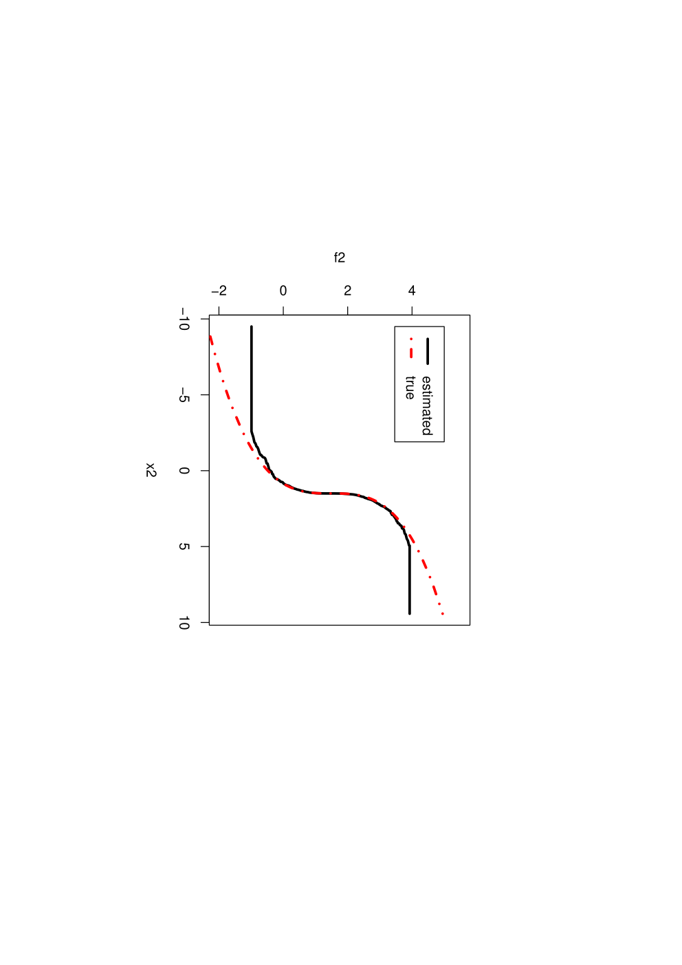
For sample size n=1000n=1000, we plot the estimated transformations for three of the variables in Figure 5. It is clear that Winsorization plays a significant role for the power transformation. This is intuitive due to the high skewness of the nonparanormal distribution resulting from the power transformations.

cdf power linear
Refer to caption Refer to caption Refer to caption
Figure 5: Estimated transformations for the first three variables.
cdf power linear
Refer to caption Refer to caption Refer to caption
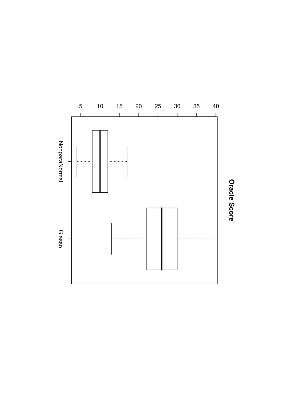
Figure 6: Boxplots of the oracle scores for n=1000,500,200n=1000,500,200 (top, center, bottom).

6.A.3 Quantitative comparison

To evaluate the performance for structure estimation quantitatively, we use false positive and false negative rates. Let G=(V,E)G=(V,E) be a pp-dimensional graph (which has at most (p2)\binom{p}{2} edges) in which there are |E|=r|E|=r edges, and let G^λ=(V,E^λ)\widehat{G}^{\lambda}=(V,\widehat{E}^{\lambda}) be an estimated graph using the regularization parameter λ\lambda. The number of false positives at λ\lambda is

FP(λ)≡number of edges in E^λ not in E\displaystyle\mathrm{FP(\lambda)}\equiv\text{number of edges in $\widehat{E}^{\lambda}$ not in $E$}

The number of false negatives at λ\lambda is defined as

FN(λ)≡number of edges in E not in E^λ.\displaystyle\mathrm{FN(\lambda)}\equiv\text{number of edges in $E$ not in $\widehat{E}^{\lambda}$}.

The oracle regularization level λ∗\lambda^{*} is then

λ∗=arg minλ∈Λ⁡{FP⁡(λ)+FN⁡(λ)}.\displaystyle\lambda^{*}=\mathop{\text{arg\,min}}_{\lambda\in\Lambda}\left\{\mathrm{FP(\lambda)}+\mathrm{FN(\lambda)}\right\}.

The oracle score is FP⁡(λ∗)+FN⁡(λ∗)\mathrm{FP}(\lambda^{*})+\mathrm{FN}(\lambda^{*}). Figure 6 shows boxplots of the oracle scores for the two methods, calculated using 100 simulations.

To illustrate the overall performance of these two methods over the full paths, ROC curves are shown in Figure 7, using

(1−FN⁡(λ)r,1−FP⁡(λ)(p2)−r).\displaystyle\left(1-\frac{\mathrm{FN}(\lambda)}{r},1-\frac{\mathrm{FP}(\lambda)}{\binom{p}{2}-r}\right).

The curves clearly show how the performance of both methods improves with sample size, and that the nonparanormal is superior to the Gaussian model in most cases.

cdf power linear
Refer to caption Refer to caption Refer to caption
Figure 7: ROC curves for sample sizes n=1000,500,200n=1000,500,200 (top, middle, bottom).

Let FPE≡FP⁡(λ∗)\mathrm{FPE}\equiv\mathrm{FP}(\lambda^{*}) and FNE≡FN⁡(λ∗)\mathrm{FNE}\equiv\mathrm{FN}(\lambda^{*}), Tables 1, 2, and 3 provide numerical comparisons of both methods on datasets with different transformations, where we repeat the experiments 100 times and report the average FPE and FNE\mathrm{FNE} values with the corresponding standard deviations. It’s clear from the tables that the nonparanormal achieves significantly smaller errors than the glasso if the true distribution of the data is not multivariate Gaussian and achieves comparable performance as the glasso when the true distribution is exactly multivariate Gaussian.

Table 1: Quantitative comparison on the dataset using the cdf transformation
Nonparanormal    glasso
n\displaystyle n FPE{\rm FPE} (sd⁡(FPE)){\rm(sd(FPE))} FNE{\rm FNE} (sd⁡(FNE)){\rm(sd(FNE))} FPE{\rm FPE} (sd⁡(FPE)){\rm(sd(FPE))} FNE{\rm FNE} (sd⁡(FNE)){\rm(sd(FNE))}
1000\displaystyle 1000 0.100.10 (0.3333)(0.3333) 0.050.05 (0.2190)(0.2190) 3.733.73 (2.3904)(2.3904) 7.247.24 (3.2910)(3.2910)
900\displaystyle 900 0.180.18 (0.5389)(0.5389) 0.160.16 (0.4197)(0.4197) 3.313.31 (2.4358)(2.4358) 8.948.94 (3.2808)(3.2808)
800\displaystyle 800 0.160.16 (0.5069)(0.5069) 0.230.23 (0.5659)(0.5659) 3.803.80 (2.9439)(2.9439) 9.919.91 (3.4789)(3.4789)
700\displaystyle 700 0.260.26 (0.6295)(0.6295) 0.430.43 (0.7420)(0.7420) 3.453.45 (2.5519)(2.5519) 12.2612.26 (3.5862)(3.5862)
600\displaystyle 600 0.330.33 (0.6039)(0.6039) 0.410.41 (0.6371)(0.6371) 3.313.31 (2.8804)(2.8804) 14.2514.25 (4.0735)(4.0735)
500\displaystyle 500 0.580.58 (0.9658)(0.9658) 1.101.10 (1.0396)(1.0396) 3.183.18 (2.9211)(2.9211) 17.5417.54 (4.4368)(4.4368)
400\displaystyle 400 0.710.71 (1.0569)(1.0569) 1.521.52 (1.2016)(1.2016) 1.581.58 (2.3535)(2.3535) 21.1821.18 (4.9855)(4.9855)
300\displaystyle 300 1.371.37 (1.4470)(1.4470) 2.972.97 (2.0123)(2.0123) 0.670.67 (1.6940)(1.6940) 23.1423.14 (5.0232)(5.0232)
200\displaystyle 200 2.032.03 (1.9356)(1.9356) 7.137.13 (3.4514)(3.4514) 0.010.01 (0.1000)(0.1000) 24.0324.03 (4.9816)(4.9816)
Table 2: Quantitative comparison on the dataset using the power transformation
Nonparanormal    glasso
n\displaystyle n FPE{\rm FPE} (sd⁡(FPE)){\rm(sd(FPE))} FNE{\rm FNE} (sd⁡(FNE)){\rm(sd(FNE))} FPE{\rm FPE} (sd⁡(FPE)){\rm(sd(FPE))} FNE{\rm FNE} (sd⁡(FNE)){\rm(sd(FNE))}
1000\displaystyle 1000 0.270.27 (0.7086)(0.7086) 0.350.35 (0.6571)(0.6571) 2.892.89 (1.9482)(1.9482) 4.974.97 (2.9213)(2.9213)
900\displaystyle 900 0.380.38 (0.6783)(0.6783) 0.410.41 (0.6210)(0.6210) 2.982.98 (2.3697)(2.3697) 5.995.99 (3.0467)(3.0467)
800\displaystyle 800 0.250.25 (0.5751)(0.5751) 0.730.73 (0.8270)(0.8270) 4.104.10 (2.7834)(2.7834) 6.396.39 (3.3571)(3.3571)
700\displaystyle 700 0.690.69 (0.9067)(0.9067) 0.900.90 (1.0200)(1.0200) 4.424.42 (2.8891)(2.8891) 8.808.80 (3.9848)(3.9848)
600\displaystyle 600 0.920.92 (1.2282)(1.2282) 1.591.59 (1.5314)(1.5314) 4.644.64 (3.3830)(3.3830) 10.5810.58 (4.2168)(4.2168)
500\displaystyle 500 1.171.17 (1.3413)(1.3413) 2.562.56 (2.3325)(2.3325) 4.004.00 (2.9644)(2.9644) 13.0913.09 (4.4903)(4.4903)
400\displaystyle 400 1.881.88 (1.6470)(1.6470) 4.974.97 (2.7687)(2.7687) 3.143.14 (3.4699)(3.4699) 17.8717.87 (4.7750)(4.7750)
300\displaystyle 300 2.972.97 (2.4181)(2.4181) 7.857.85 (3.5572)(3.5572) 1.361.36 (2.3805)(2.3805) 21.2421.24 (4.7505)(4.7505)
200\displaystyle 200 2.822.82 (2.6184)(2.6184) 14.5314.53 (4.3378)(4.3378) 0.370.37 (0.9914)(0.9914) 24.0124.01 (5.0940)(5.0940)
Table 3: Quantitative comparison on the dataset without any transformation
Nonparanormal    glasso
n\displaystyle n FPE{\rm FPE} (sd⁡(FPE)){\rm(sd(FPE))} FNE{\rm FNE} (sd⁡(FNE)){\rm(sd(FNE))} FPE{\rm FPE} (sd⁡(FPE)){\rm(sd(FPE))} FNE{\rm FNE} (sd⁡(FNE)){\rm(sd(FNE))}
1000\displaystyle 1000 0.100.10 (0.3333)(0.3333) 0.050.05 (0.2190)(0.2190) 0.090.09 (0.3208)(0.3208) 0.060.06 (0.2386)(0.2386)
900\displaystyle 900 0.240.24 (0.7537)(0.7537) 0.140.14 (0.4025)(0.4025) 0.220.22 (0.6447)(0.6447) 0.150.15 (0.4113)(0.4113)
800\displaystyle 800 0.170.17 (0.4277)(0.4277) 0.160.16 (0.3949)(0.3949) 0.160.16 (0.4431)(0.4431) 0.190.19 (0.4191)(0.4191)
700\displaystyle 700 0.250.25 (0.6871)(0.6871) 0.330.33 (0.8534)(0.8534) 0.290.29 (0.8201)(0.8201) 0.270.27 (0.7501)(0.7501)
600\displaystyle 600 0.370.37 (0.7740)(0.7740) 0.360.36 (0.7456)(0.7456) 0.360.36 (0.7722)(0.7722) 0.370.37 (0.6459)(0.6459)
500\displaystyle 500 0.280.28 (0.5874)(0.5874) 0.460.46 (0.7442)(0.7442) 0.250.25 (0.5573)(0.5573) 0.450.45 (0.6571)(0.6571)
400\displaystyle 400 0.550.55 (0.8453)(0.8453) 1.371.37 (1.2605)(1.2605) 0.470.47 (0.7713)(0.7713) 1.351.35 (1.2502)(1.2502)
300\displaystyle 300 1.241.24 (1.3715)(1.3715) 3.073.07 (1.7306)(1.7306) 0.980.98 (1.2058)(1.2058) 3.043.04 (1.8905)(1.8905)
200\displaystyle 200 1.621.62 (1.7219)(1.7219) 5.895.89 (2.7373)(2.7373) 1.551.55 (1.6779)(1.6779) 5.625.62 (2.6620)(2.6620)

6.A.4 Visualization of typical runs

Figure 8 shows typical runs for the cdf and power transformations. It’s clear that when the glasso estimates the graph incorrectly, the mistakes include both false positives and negatives.

cdf power
Refer to caption Refer to caption
Figure 8: Typical runs for the two methods for n=1000n=1000 using the cdf and power transformations. The dashed (black) lines in the symmetric difference plots indicate edges found by the glasso but not the nonparanormal, and vice-versa for the solid (red) lines.

6.B Gene microarray data

In this study, we consider a dataset based on Affymetrix GeneChip microarrays for the plant Arabidopsis thaliana, (Wille, 2004). The sample size is n=118n=118. The expression levels for each chip are pre-processed by log-transformation and standardization. A subset of 40 genes from the isoprenoid pathway are chosen, and we study the associations among them using both the paranormal and nonparanormal models. Even though these data are generally treated as multivariate Gaussian in the previous analysis (Wille, 2004), our study shows that the results of the nonparanormal and the glasso are very different over a wide range of regularization parameters. This suggests the nonparanormal could support different scientific conclusions.

6.B.1 Comparison of the regularization paths

We first compare the regularization paths of the two methods, in Figure 9. To generate the paths, we select 50 regularization parameters on an evenly spaced grid in the interval [0.16,1.2][0.16,1.2]. Although the paths for the two methods look similar, there are some subtle differences. In particular, variables become nonzero in a different order, especially when the regularization parameter is in the range λ∈[0.2,0.3]\lambda\in[0.2,0.3]. As shown below, these subtle differences in the paths lead to different model selection behaviors.

Refer to caption Refer to caption
Figure 9: The regularization paths of both methods on the microarray dataset.

6.B.2 Comparison of the selected graphs

Figure 11 compares the estimated graphs for the two methods at several values of the regularization parameter λ\lambda in the range [0.16,0.37][0.16,0.37]. For each λ\lambda, we show the estimated graph from the nonparanormal in the first column. In the second column we show the graph obtained by scanning the full regularization path of the glasso fit and finding the graph having the smallest symmetric difference with the nonparanormal graph. The symmetric difference graph is shown in in the third column. The closest glasso fit is different, with edges selected by the glasso not selected by the nonparanormal, and vice-versa. Several estimated transformations are plotted in Figure 11, which are are nonlinear. Interestingly, several of the differences between the fitted graphs are related to these variables.

Refer to caption Refer to caption Refer to caption
Figure 10: The nonparanormal estimated graph for three values of λ=0.2448,0.2661,0.30857\lambda=0.2448,0.2661,0.30857 (left column), the glasso estimated graph (middle) and the symmetric difference graph (right).
Refer to caption Refer to caption Refer to caption Refer to caption
Figure 11: Estimated transformations for the microarray dataset, indicating non-Gaussian marginals. The corresponding genes are among the nodes appearing in the symmetric difference graphs of Figure 11.

7 Proofs

We assume, without loss of generality from Lemma 3.3, that μj=0\mu_{j}=0 and σj=1\sigma_{j}=1 for all j=1,…,pj=1,\ldots,p. Thus, define f~j​(x)≡Φ−1​(F~j​(x))\widetilde{f}_{j}(x)\equiv\Phi^{-1}(\widetilde{F}_{j}(x)) and fj​(x)≡Φ−1​(Fj​(x)){f}_{j}(x)\equiv\Phi^{-1}({F}_{j}(x)), and let gj≡fj−1g_{j}\equiv f_{j}^{-1}.

7.A Proof of Theorem 5.1

We start with some useful lemmas; the first is from Abramovich et al. (2006).

Lemma 7.1

. ​(Gaussian Distribution function vs. Quantile function) Let Φ\Phi and ϕ\phi denote the distribution and density functions of a standard Gaussian random variable. Then

ϕ⁡(t)2​t≤1−Φ⁡(t)≤ϕ⁡(t)t​if​t≥1\displaystyle\frac{\phi(t)}{2t}\leq 1-\Phi(t)\leq\frac{\phi(t)}{t}~~\mathrm{if}~t\geq 1 (18)

and

(Φ−1)′​(η)=1ϕ​(Φ−1​(η)).\displaystyle(\Phi^{-1})^{\prime}(\eta)=\frac{1}{\phi\left(\Phi^{-1}(\eta)\right)}. (19)

Also, for η≥0.99\eta\geq 0.99, we have

Φ−1​(η)=2​log⁡(11−η)−r⁡(η)\displaystyle\Phi^{-1}(\eta)=\displaystyle\sqrt{2\log\left(\frac{1}{1-\eta}\right)}-r(\eta) (20)

where r⁡(η)∈[0,1.5]r(\eta)\in[0,1.5].

Lemma 7.2

. ​(Distribution function of the transformed random variable) For any α∈(−∞,∞)\alpha\in(-\infty,\infty)

Φ−1​(Fj​(gj​(α​log⁡n)))=α​log⁡n.\displaystyle\Phi^{-1}\left(F_{j}\left(g_{j}(\alpha\sqrt{\log n})\right)\right)=\alpha\sqrt{\log n}.

Proof. The statement follows from

Fj​(t)=ℙ⁡(Xj≤t)=ℙ⁡(gj​(Zj)≤t)=ℙ⁡(Zj≤gj−1​(t))=Φ⁡(gj−1​(t)).\displaystyle F_{j}(t)=\mathbb{P}(X_{j}\leq t)=\mathbb{P}(g_{j}(Z_{j})\leq t)=\mathbb{P}(Z_{j}\leq g^{-1}_{j}(t))=\Phi\left(g_{j}^{-1}(t)\right). (21)

which holds for any tt.  □\;\;\scriptstyle\Box

Lemma 7.3

. ​(Gaussian maximal inequality) Let W1,…,WnW_{1},\ldots,W_{n} be independently and identically distributed standard Gaussian random variables. Then for any α>0\alpha>0

ℙ⁡(max1≤i≤n⁡Wi>α​log⁡n)≤1nα/2−1.\displaystyle\mathbb{P}\left(\max_{1\leq i\leq n}W_{i}>\sqrt{\alpha\log n}\right)\leq\frac{1}{n^{\alpha/2-1}}.

Proof. Using Mill’s inequality, we have

ℙ⁡(max1≤i≤n⁡Wi>α​log⁡n)≤∑i=1nℙ⁡(Wi>α​log⁡n)≤n​ϕ⁡(α​log⁡n)α​log⁡n=1nα/2−1​2​π​α​log⁡n,\displaystyle\mathbb{P}\left(\max_{1\leq i\leq n}W_{i}>\sqrt{\alpha\log n}\right)\leq\sum_{i=1}^{n}\mathbb{P}\left(W_{i}>\sqrt{\alpha\log n}\right)\leq n\frac{\phi(\sqrt{\alpha\log n})}{\sqrt{\alpha\log n}}=\frac{1}{n^{\alpha/2-1}\sqrt{2\pi\alpha\log n}},

from which the result follows.  □\;\;\scriptstyle\Box

Lemma 7.4

.  For any α>0\alpha>0 that satisfies 1−δn−Φ⁡(α​log⁡n)>01-\delta_{n}-\Phi\left(\sqrt{\alpha\log n}\right)>0 for all nn, we have

ℙ[F^j(gj(α​log⁡n))>1−δn]≤exp{−2n(1−δn−Φ(α​log⁡n))2}.\displaystyle\mathbb{P}\left[\widehat{F}_{j}\left(g_{j}\left(\sqrt{\alpha\log n}\right)\right)>1-\delta_{n}\right]\leq\exp\left\{-2n\left(1-\delta_{n}-\Phi\left(\sqrt{\alpha\log n}\right)\right)^{2}\right\}. (22)

and

ℙ[F^j(gj(−α​log⁡n))<δn]≤exp{−2n(1−δn−Φ(α​log⁡n))2}.\displaystyle\mathbb{P}\left[\widehat{F}_{j}\left(g_{j}\left(-\sqrt{\alpha\log n}\right)\right)<\delta_{n}\right]\leq\exp\left\{-2n\left(1-\delta_{n}-\Phi\left(\sqrt{\alpha\log n}\right)\right)^{2}\right\}. (23)

Proof. Using Hoeffding’s inequality,

ℙ[F^j(gj(α​log⁡n))>1−δn]\displaystyle{\mathbb{P}}\left[\widehat{F}_{j}\left(g_{j}\left(\sqrt{\alpha\log n}\right)\right)>1-\delta_{n}\right]
=\displaystyle= ℙ[F^j(gj(α​log⁡n))−Fj(gj(α​log⁡n))>1−δn−Fj(gj(α​log⁡n))]\displaystyle{\mathbb{P}}\left[\widehat{F}_{j}\left(g_{j}\left(\sqrt{\alpha\log n}\right)\right)-{F}_{j}\left(g_{j}\left(\sqrt{\alpha\log n}\right)\right)>1-\delta_{n}-{F}_{j}\left(g_{j}\left(\sqrt{\alpha\log n}\right)\right)\right]
≤\displaystyle\leq exp⁡{−2​n​(1−δn−Fj​(gj​(α​log⁡n)))2}.\displaystyle\exp\left\{-2n\left(1-\delta_{n}-{F}_{j}\left(g_{j}\left(\sqrt{\alpha\log n}\right)\right)\right)^{2}\right\}.

Equation (22) then follows from equation (21). The proof of equation (23) uses the same argument.  □\;\;\scriptstyle\Box

Now let M>2M>2 be some constant and set β=12\displaystyle\beta=\frac{1}{2}. We split the interval

[gj​(−M​log⁡n),gj​(M​log⁡n)]\left[g_{j}(-\sqrt{M\log n}),g_{j}(\sqrt{M\log n})\right]

into two parts, the middle

ℳn≡(gj​(−β​log⁡n),gj​(β​log⁡n))\displaystyle{\mathcal{M}}_{n}\equiv\left(g_{j}\left(-\sqrt{\beta\log n}\right),g_{j}\left(\sqrt{\beta\log n}\right)\right)

and ends

ℰn≡[gj​(−M​log⁡n),gj​(−β​log⁡n)]∪[gj​(β​log⁡n),gj​(M​log⁡n)].\displaystyle{\mathcal{E}}_{n}\equiv\left[g_{j}\left(-\sqrt{M\log n}\right),g_{j}\left(-\sqrt{\beta\log n}\right)\right]\cup\left[g_{j}\left(\sqrt{\beta\log n}\right),g_{j}\left(\sqrt{M\log n}\right)\right].

The behaviors of the function estimates in these two regions is different, and so we first establish bounds on the probability that a sample can fall in the end region ℰn{\mathcal{E}}_{n}.

Lemma 7.5

.  Let A≡2π​(M−β)\displaystyle A\equiv\sqrt{\frac{2}{\pi}}(\sqrt{M}-\sqrt{\beta}). Then

ℙ⁡(X1​j∈ℰn)≤A​log⁡nnβ,∀j∈{1,…,p}.\displaystyle\mathbb{P}\left(X_{1j}\in{\mathcal{E}}_{n}\right)\leq A\sqrt{\frac{\log n}{n^{\beta}}},~~\forall j\in\{1,\ldots,p\}.

Proof. Using equation (21) and the mean value theorem, we have

ℙ⁡(X1​j∈ℰn)\displaystyle\mathbb{P}\left(X_{1j}\in{\mathcal{E}}_{n}\right)
=\displaystyle= ℙ⁡(X1​j∈[gj​(β​log⁡n),gj​(M​log⁡n)])+ℙ⁡(X1​j∈[gj​(−M​log⁡n),gj​(−β​log⁡n)])\displaystyle\mathbb{P}\left(X_{1j}\in\left[g_{j}(\sqrt{\beta\log n}),g_{j}(\sqrt{M\log n})\right]\right)+\mathbb{P}\left(X_{1j}\in\left[g_{j}(-\sqrt{M\log n}),g_{j}(-\sqrt{\beta\log n})\right]\right)
=\displaystyle= Fj​(gj​(M​log⁡n))−Fj​(gj​(β​log⁡n))+Fj​(gj​(−β​log⁡n))−Fj​(gj​(−M​log⁡n))\displaystyle F_{j}\left(g_{j}(\sqrt{M\log n})\right)-F_{j}\left(g_{j}(\sqrt{\beta\log n})\right)+F_{j}\left(g_{j}(-\sqrt{\beta\log n})\right)-F_{j}\left(g_{j}(-\sqrt{M\log n})\right)
=\displaystyle= 2​(Φ​(M​log⁡n)−Φ​(β​log⁡n))\displaystyle 2\left(\Phi(\sqrt{M\log n})-\Phi(\sqrt{\beta\log n})\right)
≤\displaystyle\leq 2​ϕ​(β​log⁡n)​(M​log⁡n−β​log⁡n).\displaystyle 2\phi\left(\sqrt{\beta\log n}\right)\left(\sqrt{M\log n}-\sqrt{\beta\log n}\right).

The result of the lemma follows directly.  □\;\;\scriptstyle\Box

We next bound the error of the Winsorized estimate of a component function over the end region.

Lemma 7.6

.  For all nn, we have

supt∈ℰn|Φ−1​(F~j​(t))−Φ−1​(Fj​(t))|<2​(M+2)​log⁡n,∀j∈{1,…,p}.\displaystyle\sup_{t\in{\mathcal{E}}_{n}}\left|\Phi^{-1}(\widetilde{F}_{j}(t))-\Phi^{-1}\left(F_{j}(t)\right)\right|<\sqrt{2(M+2)\log n},~~\forall j\in\{1,\ldots,p\}.

Proof. From Lemma 7.2 and the definition of ℰn{\mathcal{E}}_{n}, we have

supt∈ℰn|Φ−1​(Fj​(t))|∈[0,M​log⁡n].\sup_{t\in{\mathcal{E}}_{n}}\left|\Phi^{-1}\left(F_{j}(t)\right)\right|\in\left[0,\sqrt{M\log n}\right].

Given the fact that δn=14​n1/4​π​log⁡n\delta_{n}=\displaystyle\frac{1}{4n^{1/4}\sqrt{\pi\log n}}, we have F~j​(t)∈(1n,1−1n)\widetilde{F}_{j}(t)\in\displaystyle\left(\frac{1}{n},1-\frac{1}{n}\right). Therefore, from equation (20),

supt∈ℰn|Φ−1​(F~j​(t))|∈[0,2​log⁡n).\displaystyle\sup_{t\in{\mathcal{E}}_{n}}\left|\Phi^{-1}\left(\widetilde{F}_{j}(t)\right)\right|\in\left[0,\sqrt{2\log n}\right).

The result follows from the triangle inequality and M+2≤2​(M+2)\sqrt{M}+\sqrt{2}\leq\sqrt{2(M+2)}.  □\;\;\scriptstyle\Box

Now for any ϵ>0\epsilon>0, we have

ℙ⁡(maxj,k⁡|Sn​(f~)j​k−Sn​(f)j​k|>ϵ)\displaystyle\mathbb{P}\left(\max_{j,k}\left|S_{n}(\widetilde{f})_{jk}-S_{n}(f)_{jk}\right|>\epsilon\right)
=\displaystyle= ℙ⁡(maxj,k⁡|1n​∑i=1n{f~j​(Xi​j)​f~k​(Xi​k)−fj​(Xi​j)​fk​(Xi​k)−μn​(f~j)​μn​(f~k)+μn​(fj)​μn​(fk)}|>ϵ)\displaystyle\mathbb{P}\left(\max_{j,k}\left|\frac{1}{n}\sum_{i=1}^{n}\left\{\widetilde{f}_{j}(X_{ij})\widetilde{f}_{k}(X_{ik})-f_{j}(X_{ij})f_{k}(X_{ik})-\mu_{n}(\widetilde{f}_{j})\mu_{n}(\widetilde{f}_{k})+\mu_{n}(f_{j})\mu_{n}(f_{k})\right\}\right|>\epsilon\right)
≤\displaystyle\leq ℙ⁡(maxj,k⁡|1n​∑i=1n(f~j​(Xi​j)​f~k​(Xi​k)−fj​(Xi​j)​fk​(Xi​k))|>ϵ2)\displaystyle\mathbb{P}\left(\max_{j,k}\left|\frac{1}{n}\sum_{i=1}^{n}\left(\widetilde{f}_{j}(X_{ij})\widetilde{f}_{k}(X_{ik})-f_{j}(X_{ij})f_{k}(X_{ik})\right)\right|>\frac{\epsilon}{2}\right)
+ℙ⁡(maxj,k⁡|μn​(f~j)​μn​(f~k)−μn​(fj)​μn​(fk)|>ϵ2).\displaystyle+\;\mathbb{P}\left(\max_{j,k}\left|\mu_{n}(\widetilde{f}_{j})\mu_{n}(\widetilde{f}_{k})-\mu_{n}(f_{j})\mu_{n}(f_{k})\right|>\frac{\epsilon}{2}\right).

We only need to analyze the rate for the first term above, since the second one is of higher order (Cai et al., 2008). Let

Δi​(j,k)≡f~j​(Xi​j)​f~k​(Xi​k)−fj​(Xi​j)​fk​(Xi​k)\displaystyle\Delta_{i}(j,k)\equiv\widetilde{f}_{j}(X_{ij})\widetilde{f}_{k}(X_{ik})-f_{j}(X_{ij})f_{k}(X_{ik})

and

Θt,s​(j,k)≡f~j​(t)​f~k​(s)−fj​(t)​fk​(s).\displaystyle\Theta_{t,s}(j,k)\equiv\widetilde{f}_{j}(t)\widetilde{f}_{k}(s)-f_{j}(t)f_{k}(s).

We define the event 𝒜n\mathcal{A}_{n} as

𝒜n≡{gj​(−M​log⁡n)≤X1​j,…,Xn​j≤gj​(M​log⁡n),j=1,…,p}.\displaystyle\mathcal{A}_{n}\equiv\left\{g_{j}\left(-\sqrt{M\log n}\right)\leq X_{1j},\ldots,X_{nj}\leq g_{j}\left(\sqrt{M\log n}\right),j=1,\ldots,p\right\}.

Then

ℙ⁡(𝒜nc)≤p​ℙ​(mini⁡fj​(Xi​j)<−M​log⁡n)+p​ℙ​(maxi⁡fj​(Xi​j)>M​log⁡n)≤c1​nξnM/2−1.\displaystyle\mathbb{P}(\mathcal{A}_{n}^{c})\leq p\mathbb{P}\left(\min_{i}f_{j}\left(X_{ij}\right)<-\sqrt{M\log n}\right)+p\mathbb{P}\left(\max_{i}f_{j}\left(X_{ij}\right)>\sqrt{M\log n}\right)\leq\frac{c_{1}n^{\xi}}{n^{M/2-1}}.

with c1c_{1} as a generic positive constant. Therefore

ℙ⁡(maxj,k⁡|1n​∑i=1nΔi​(j,k)|>ϵ)≤ℙ⁡(maxj,k⁡|1n​∑i=1nΔi​(j,k)|>ϵ,𝒜n)\displaystyle\mathbb{P}\left(\max_{j,k}\left|\frac{1}{n}\sum_{i=1}^{n}\Delta_{i}(j,k)\right|>\epsilon\right)\leq\mathbb{P}\left(\max_{j,k}\left|\frac{1}{n}\sum_{i=1}^{n}\Delta_{i}(j,k)\right|>\epsilon,\mathcal{A}_{n}\right) +\displaystyle+ ℙ⁡(𝒜nc)\displaystyle\mathbb{P}(\mathcal{A}_{n}^{c})
≤ℙ⁡(maxj,k⁡|1n​∑i=1nΔi​(j,k)|>ϵ,𝒜n)\displaystyle\leq\mathbb{P}\left(\max_{j,k}\left|\frac{1}{n}\sum_{i=1}^{n}\Delta_{i}(j,k)\right|>\epsilon,\mathcal{A}_{n}\right) +\displaystyle+ c1​nξnM/2−1.\displaystyle\frac{c_{1}n^{\xi}}{n^{M/2-1}}.

Thus, we only need to carry out our analysis on the event 𝒜n\mathcal{A}_{n}. On this event, we have the following decomposition:

ℙ⁡(maxj,k⁡|1n​∑i=1nΔi​(j,k)|>ϵ,𝒜n)\displaystyle\mathbb{P}\left(\max_{j,k}\left|\frac{1}{n}\sum_{i=1}^{n}\Delta_{i}(j,k)\right|>\epsilon,\,\mathcal{A}_{n}\right)
≤\displaystyle\leq ℙ⁡(maxj,k⁡1n​∑Xi​j∈ℳn,Xi​k∈ℳn|Δi​(j,k)|>ϵ4)+ℙ⁡(maxj,k⁡1n​∑Xi​j∈ℰn,Xi​k∈ℰn|Δi​(j,k)|>ϵ4)\displaystyle\mathbb{P}\left(\max_{j,k}\frac{1}{n}\sum_{X_{ij}\in{\mathcal{M}}_{n},X_{ik}\in{\mathcal{M}}_{n}}\left|\Delta_{i}(j,k)\right|>\frac{\epsilon}{4}\right)+\mathbb{P}\left(\max_{j,k}\frac{1}{n}\sum_{X_{ij}\in{\mathcal{E}}_{n},X_{ik}\in{\mathcal{E}}_{n}}\left|\Delta_{i}(j,k)\right|>\frac{\epsilon}{4}\right)
+ 2​ℙ​(maxj,k⁡1n​∑Xi​j∈ℳn,Xi​k∈ℰn|Δi​(j,k)|>ϵ4).\displaystyle+\;2\mathbb{P}\left(\max_{j,k}\frac{1}{n}\sum_{X_{ij}\in{\mathcal{M}}_{n},X_{ik}\in{\mathcal{E}}_{n}}\left|\Delta_{i}(j,k)\right|>\frac{\epsilon}{4}\right).

We now analyze each of these terms separately.

Lemma 7.7

.  On the event 𝒜n\mathcal{A}_{n}, let β=1/2\beta=1/2 and ϵ≥C⁡(M,ξ)​log⁡p​log2​nn1/2\displaystyle\epsilon\geq C(M,\xi)\sqrt{\frac{\log p\log^{2}n}{n^{1/2}}}, then

ℙ⁡(maxj,k⁡1n​∑Xi​j∈ℰn,Xi​k∈ℰn|Δi​(j,k)|>ϵ4)=o⁡(1).\displaystyle\mathbb{P}\left(\max_{j,k}\frac{1}{n}\sum_{X_{ij}\in{\mathcal{E}}_{n},X_{ik}\in{\mathcal{E}}_{n}}\left|\Delta_{i}(j,k)\right|>\frac{\epsilon}{4}\right)=o(1).

Proof. We define

θ1≡nβ/2​ϵ8​A​log⁡n\displaystyle\theta_{1}\equiv\frac{n^{\beta/2}\epsilon}{8A\sqrt{\log n}}

with the same parameter AA as in Lemma 7.5. Such a θ1\theta_{1} guarantees that

n​ϵ4​θ1−n​A​log⁡nnβ=n​A​log⁡nnβ>0.\displaystyle\frac{n\epsilon}{4\theta_{1}}-nA\sqrt{\frac{\log n}{n^{\beta}}}=nA\sqrt{\frac{\log n}{n^{\beta}}}>0.

By Lemma 7.5, we have

ℙ(1n∑i=1n𝟏{Xi​j∈ℰn,Xi​k∈ℰn}>ϵ4​θ1)≤ℙ(∑i=1n𝟏{Xi​j∈ℰn}>n​ϵ4​θ1)\displaystyle\mathbb{P}\left(\frac{1}{n}\sum_{i=1}^{n}\mathbf{1}_{\{X_{ij}\in{\mathcal{E}}_{n},X_{ik}\in{\mathcal{E}}_{n}\}}>\frac{\epsilon}{4\theta_{1}}\right)\;\leq\;\mathbb{P}\left(\sum_{i=1}^{n}\mathbf{1}_{\{X_{ij}\in{\mathcal{E}}_{n}\}}>\frac{n\epsilon}{4\theta_{1}}\right)
=\displaystyle= ℙ(∑i=1n(𝟏{Xi​j∈ℰn}−ℙ(X1​j∈ℰn))>n​ϵ4​θ1−nℙ(X1​j∈ℰn))\displaystyle\mathbb{P}\left(\sum_{i=1}^{n}\left(\mathbf{1}_{\{X_{ij}\in{\mathcal{E}}_{n}\}}-\mathbb{P}\left(X_{1j}\in{\mathcal{E}}_{n}\right)\right)>\frac{n\epsilon}{4\theta_{1}}-n\mathbb{P}\left(X_{1j}\in{\mathcal{E}}_{n}\right)\right)
≤\displaystyle\leq ℙ(∑i=1n(𝟏{Xi​j∈ℰn}−ℙ(X1​j∈ℰn))>n​ϵ4​θ1−nAlog⁡nnβ).\displaystyle\mathbb{P}\left(\sum_{i=1}^{n}\left(\mathbf{1}_{\{X_{ij}\in{\mathcal{E}}_{n}\}}-\mathbb{P}\left(X_{1j}\in{\mathcal{E}}_{n}\right)\right)>\frac{n\epsilon}{4\theta_{1}}-nA\sqrt{\frac{\log n}{n^{\beta}}}\right).

Using the Bernstein’s inequality, for β=12\beta=\displaystyle\frac{1}{2},

ℙ⁡(1n​∑i=1n𝟏{Xi​j∈ℰn,Xi​k∈ℰn}>ϵ4​θ1)\displaystyle\mathbb{P}\left(\frac{1}{n}\sum_{i=1}^{n}\mathbf{1}_{\{X_{ij}\in{\mathcal{E}}_{n},X_{ik}\in{\mathcal{E}}_{n}\}}>\frac{\epsilon}{4\theta_{1}}\right) ≤\displaystyle\leq ℙ(∑i=1n(𝟏{Xi​j∈ℰn}−ℙ(X1​j∈ℰn))>nAlog⁡nnβ)\displaystyle\mathbb{P}\left(\sum_{i=1}^{n}\left(\mathbf{1}_{\{X_{ij}\in{\mathcal{E}}_{n}\}}-\mathbb{P}\left(X_{1j}\in{\mathcal{E}}_{n}\right)\right)>nA\sqrt{\frac{\log n}{n^{\beta}}}\right)
≤\displaystyle\leq exp⁡(−c1​n2−β​log⁡nc2​n1−β/2​log⁡n+c3​n1−β/2​log⁡n)=o⁡(1),\displaystyle\exp\left(-\frac{c_{1}n^{2-\beta}\log n}{c_{2}n^{1-\beta/2}\sqrt{\log n}+c_{3}n^{1-\beta/2}\sqrt{\log n}}\right)=o(1),

where c1,c2,c3>0c_{1},c_{2},c_{3}>0 are generic constants.

Therefore,

ℙ⁡(maxj,k⁡1n​∑Xi​j∈ℰn,Xi​k∈ℰn|Δi​(j,k)|>ϵ4)\displaystyle\mathbb{P}\left(\max_{j,k}\frac{1}{n}\sum_{X_{ij}\in{\mathcal{E}}_{n},X_{ik}\in{\mathcal{E}}_{n}}\left|\Delta_{i}(j,k)\right|>\frac{\epsilon}{4}\right)
=\displaystyle= ℙ(maxj,k1n∑Xi​j∈ℰn,Xi​k∈ℰn|Δi(j,k)|>ϵ4,maxj,ksupt∈ℰn,s∈ℰn|Θt,s(j,k)|>θ1)\displaystyle\mathbb{P}\left(\max_{j,k}\frac{1}{n}\sum_{X_{ij}\in{\mathcal{E}}_{n},X_{ik}\in{\mathcal{E}}_{n}}\left|\Delta_{i}(j,k)\right|>\frac{\epsilon}{4},\max_{j,k}\sup_{t\in{\mathcal{E}}_{n},s\in{\mathcal{E}}_{n}}\left|\Theta_{t,s}(j,k)\right|>\theta_{1}\right)
+ℙ(maxj,k1n∑Xi​j∈ℰn,Xi​k∈ℰn|Δi(j,k)|>ϵ4,maxj,ksupt∈ℰn,s∈ℰn|Θt,s(j,k)|≤θ1)\displaystyle~+\mathbb{P}\left(\max_{j,k}\frac{1}{n}\sum_{X_{ij}\in{\mathcal{E}}_{n},X_{ik}\in{\mathcal{E}}_{n}}\left|\Delta_{i}(j,k)\right|>\frac{\epsilon}{4},\max_{j,k}\sup_{t\in{\mathcal{E}}_{n},s\in{\mathcal{E}}_{n}}\left|\Theta_{t,s}(j,k)\right|\leq\theta_{1}\right)
≤\displaystyle\leq ℙ⁡(max⁡supt∈ℰn,s∈ℰnj,k⁡|Θt,s​(j,k)|>θ1)+ℙ⁡(1n​∑i=1n𝟏{Xi​j∈ℰn,Xi​k∈ℰn}>ϵ4​θ1)\displaystyle\mathbb{P}\left(\max_{j,k}\sup_{t\in{\mathcal{E}}_{n},s\in{\mathcal{E}}_{n}}\left|\Theta_{t,s}(j,k)\right|>\theta_{1}\right)+\mathbb{P}\left(\frac{1}{n}\sum_{i=1}^{n}\mathbf{1}_{\{X_{ij}\in{\mathcal{E}}_{n},X_{ik}\in{\mathcal{E}}_{n}\}}>\frac{\epsilon}{4\theta_{1}}\right)
=\displaystyle= ℙ⁡(max⁡supt∈ℰn,s∈ℰnj,k⁡|Θt,s​(j,k)|>θ1)+o⁡(1).\displaystyle\mathbb{P}\left(\max_{j,k}\sup_{t\in{\mathcal{E}}_{n},s\in{\mathcal{E}}_{n}}\left|\Theta_{t,s}(j,k)\right|>\theta_{1}\right)+o(1).

Now, we analyze the first term

ℙ⁡(max⁡supt∈ℰn,s∈ℰnj,k⁡|Θt,s​(j,k)|>θ1)\displaystyle\mathbb{P}\left(\max_{j,k}\sup_{t\in{\mathcal{E}}_{n},s\in{\mathcal{E}}_{n}}\left|\Theta_{t,s}(j,k)\right|>\theta_{1}\right) ≤\displaystyle\leq p2​ℙ​(supt∈ℰn,s∈ℰn|Θt,s​(j,k)|>θ1)\displaystyle p^{2}\mathbb{P}\left(\sup_{t\in{\mathcal{E}}_{n},s\in{\mathcal{E}}_{n}}\left|\Theta_{t,s}(j,k)\right|>\theta_{1}\right)
=\displaystyle= p2​ℙ​(supt∈ℰn,s∈ℰn|f~j​(t)​f~k​(s)−fj​(t)​fk​(s)|>θ1).\displaystyle p^{2}\mathbb{P}\left(\sup_{t\in{\mathcal{E}}_{n},s\in{\mathcal{E}}_{n}}|\widetilde{f}_{j}(t)\widetilde{f}_{k}(s)-f_{j}(t)f_{k}(s)|>\theta_{1}\right).

By adding and subtracting terms fj​(t)f_{j}(t) and fs​(t)f_{s}(t), we have

ℙ⁡(supt∈ℰn,s∈ℰn|f~j​(t)​f~k​(s)−fj​(t)​fk​(s)|>θ1)\displaystyle\mathbb{P}\left(\sup_{t\in{\mathcal{E}}_{n},s\in{\mathcal{E}}_{n}}|\widetilde{f}_{j}(t)\widetilde{f}_{k}(s)-f_{j}(t)f_{k}(s)|>\theta_{1}\right)
≤\displaystyle\leq ℙ⁡(supt∈ℰn,s∈ℰn|(f~j​(t)−fj​(t))​(f~k​(s)−fk​(s))|>θ13)\displaystyle\mathbb{P}\left(\sup_{t\in{\mathcal{E}}_{n},s\in{\mathcal{E}}_{n}}|(\widetilde{f}_{j}(t)-f_{j}(t))(\widetilde{f}_{k}(s)-f_{k}(s))|>\frac{\theta_{1}}{3}\right)
+ℙ⁡(supt∈ℰn,s∈ℰn|(f~j​(t)−fj​(t))|⋅|fk​(s)|>θ13)\displaystyle+~\mathbb{P}\left(\sup_{t\in{\mathcal{E}}_{n},s\in{\mathcal{E}}_{n}}|(\widetilde{f}_{j}(t)-f_{j}(t))|\cdot|f_{k}(s)|>\frac{\theta_{1}}{3}\right)
+ℙ⁡(supt∈ℰn,s∈ℰn|(f~k​(s)−fk​(s))|⋅|fj​(t)|>θ13).\displaystyle+~\mathbb{P}\left(\sup_{t\in{\mathcal{E}}_{n},s\in{\mathcal{E}}_{n}}|(\widetilde{f}_{k}(s)-f_{k}(s))|\cdot|f_{j}(t)|>\frac{\theta_{1}}{3}\right).

The first term can further be decomposed to be

ℙ⁡(supt∈ℰn,s∈ℰn|(f~j​(t)−fj​(t))​(f~k​(s)−fk​(s))|>θ13)\displaystyle\mathbb{P}\left(\sup_{t\in{\mathcal{E}}_{n},s\in{\mathcal{E}}_{n}}|(\widetilde{f}_{j}(t)-f_{j}(t))(\widetilde{f}_{k}(s)-f_{k}(s))|>\frac{\theta_{1}}{3}\right)
≤\displaystyle\leq ℙ⁡(supt∈ℰn|(f~j​(t)−fj​(t))|>θ13)+ℙ⁡(sups∈ℰn|(f~k​(s)−fk​(s))|>θ13).\displaystyle\mathbb{P}\left(\sup_{t\in{\mathcal{E}}_{n}}|(\widetilde{f}_{j}(t)-f_{j}(t))|>\sqrt{\frac{\theta_{1}}{3}}\right)+\mathbb{P}\left(\sup_{s\in{\mathcal{E}}_{n}}|(\widetilde{f}_{k}(s)-f_{k}(s))|>\sqrt{\frac{\theta_{1}}{3}}\right).

Also, from the definition of ℰn\mathcal{E}_{n}, we have

supt∈ℰn|fj​(t)|=supt∈ℰn|gj−1​(t)|≤M​log⁡n.\displaystyle\sup_{t\in{\mathcal{E}}_{n}}|f_{j}(t)|=\sup_{t\in{\mathcal{E}}_{n}}\left|g_{j}^{-1}(t)\right|\leq\sqrt{M\log n}.

Since ϵ≥C⁡(M,ξ)​log⁡p​log2​nn1/2\displaystyle\epsilon\geq C(M,\xi)\sqrt{\frac{\log p\log^{2}n}{n^{1/2}}}, we have

θ13=nβ/2​ϵ24​A​log⁡n≥C⁡(M,ξ)​log⁡p​log2​n24​A​log⁡n=2​(M+2)​log⁡n.\displaystyle\frac{\theta_{1}}{3}=\frac{n^{\beta/2}\epsilon}{24A\sqrt{\log n}}\geq\frac{C(M,\xi)\sqrt{\log p\log^{2}n}}{24A\sqrt{\log n}}=2(M+2)\log n.

This implies that

θ13≥2​(M+2)​log⁡n​and​θ13​M​log⁡n≥2​(M+2)​log⁡n.\displaystyle\sqrt{\frac{\theta_{1}}{3}}\geq\sqrt{2(M+2)\log n}~~\mathrm{and}~~\frac{\theta_{1}}{3\sqrt{M\log n}}\geq\sqrt{2(M+2)\log n}.

Then, from Lemma 7.6, we get

ℙ⁡(supt∈ℰn|(f~j​(t)−fj​(t))|>θ13)=0\displaystyle\mathbb{P}\left(\sup_{t\in{\mathcal{E}}_{n}}|(\widetilde{f}_{j}(t)-f_{j}(t))|>\sqrt{\frac{\theta_{1}}{3}}\right)=0

and

ℙ⁡(supt∈ℰn,s∈ℰn|(f~j​(t)−fj​(t))|⋅|fk​(s)|>θ13)=0.\displaystyle\mathbb{P}\left(\sup_{t\in{\mathcal{E}}_{n},s\in{\mathcal{E}}_{n}}|(\widetilde{f}_{j}(t)-f_{j}(t))|\cdot|f_{k}(s)|>\frac{\theta_{1}}{3}\right)=0.

The claim of the lemma then follows directly.  □\;\;\scriptstyle\Box

Remark 7.8

.  From the above analysis, we see that the data in the tails doesn’t affect the rate. Using exactly the same argument, we can also show that

ℙ⁡(maxj,k⁡1n​∑Xi​j∈ℳn,Xi​k∈ℰn|Δi​(j,k)|>ϵ4)=o⁡(1).\displaystyle\mathbb{P}\left(\max_{j,k}\frac{1}{n}\sum_{X_{ij}\in{\mathcal{M}}_{n},X_{ik}\in{\mathcal{E}}_{n}}\left|\Delta_{i}(j,k)\right|>\frac{\epsilon}{4}\right)=o(1).
Lemma 7.9

.  On the event 𝒜n\mathcal{A}_{n}, let β=1/2\beta=1/2 and ϵ≥C⁡(M,ξ)​log⁡p​log2​nn1/2\displaystyle\epsilon\geq C(M,\xi)\sqrt{\frac{\log p\log^{2}n}{n^{1/2}}}. There exist generic constants c1,c2,c3,c4c_{1},c_{2},c_{3},c_{4}, such that

ℙ⁡(maxj,k⁡1n​∑Xi​j∈ℳn,Xi​k∈ℳn|Δi​(j,k)|>ϵ4)≤c2​exp⁡(−c1​n1−β​ϵ2log⁡p​log2​n)+c3​exp⁡(−c4​n1−βlog⁡p⁡(log⁡n)).\displaystyle\mathbb{P}\left(\max_{j,k}\frac{1}{n}\sum_{X_{ij}\in{\mathcal{M}}_{n},X_{ik}\in{\mathcal{M}}_{n}}\hskip-10.0pt\left|\Delta_{i}(j,k)\right|>\frac{\epsilon}{4}\right)\leq c_{2}\exp\left(-\frac{c_{1}n^{1-\beta}\epsilon^{2}}{\log p\log^{2}n}\right)+c_{3}\exp\left(-\frac{c_{4}n^{1-\beta}}{\log p(\log n)}\right).

Proof. We have

ℙ⁡(maxj,k⁡1n​∑Xi​j∈ℳn,Xi​k∈ℳn|Δi​(j,k)|>ϵ4)≤p2​ℙ​(supt∈ℳn,s∈ℳn|f~j​(t)​f~k​(s)−fj​(t)​fk​(s)|>ϵ4)\displaystyle\mathbb{P}\left(\max_{j,k}\frac{1}{n}\sum_{X_{ij}\in{\mathcal{M}}_{n},X_{ik}\in{\mathcal{M}}_{n}}\left|\Delta_{i}(j,k)\right|>\frac{\epsilon}{4}\right)\leq p^{2}\mathbb{P}\left(\sup_{t\in{\mathcal{M}}_{n},s\in{\mathcal{M}}_{n}}|\widetilde{f}_{j}(t)\widetilde{f}_{k}(s)-f_{j}(t)f_{k}(s)|>\frac{\epsilon}{4}\right)
≤p2​ℙ​(supt∈ℳn,s∈ℳn|(f~j​(t)−fj​(t))​(f~k​(s)−fk​(s))|>ϵ12)\displaystyle\leq p^{2}\mathbb{P}\left(\sup_{t\in{\mathcal{M}}_{n},s\in{\mathcal{M}}_{n}}|(\widetilde{f}_{j}(t)-f_{j}(t))(\widetilde{f}_{k}(s)-f_{k}(s))|>\frac{\epsilon}{12}\right)
+2​p2​ℙ​(supt∈ℳn,s∈ℳn|(f~j​(t)−fj​(t))|⋅|fk​(s)|>ϵ12).\displaystyle+~2p^{2}\mathbb{P}\left(\sup_{t\in{\mathcal{M}}_{n},s\in{\mathcal{M}}_{n}}|(\widetilde{f}_{j}(t)-f_{j}(t))|\cdot|f_{k}(s)|>\frac{\epsilon}{12}\right).

Further, since

supt∈ℳn|fj​(t)|=supt∈ℳn|gj−1​(t)|=β​log⁡n\displaystyle\sup_{t\in{\mathcal{M}}_{n}}|f_{j}(t)|=\sup_{t\in{\mathcal{M}}_{n}}\left|g_{j}^{-1}(t)\right|=\sqrt{\beta\log n}

and supt∈ℳn,s∈ℳn|(f~j​(t)−fj​(t))​(f~k​(s)−fk​(s))|\displaystyle\sup_{t\in{\mathcal{M}}_{n},s\in{\mathcal{M}}_{n}}|(\widetilde{f}_{j}(t)-f_{j}(t))(\widetilde{f}_{k}(s)-f_{k}(s))| is of higher order than supt∈ℳn,s∈ℳn|(f~j​(t)−fj​(t))|⋅|fk​(s)|\sup_{t\in{\mathcal{M}}_{n},s\in{\mathcal{M}}_{n}}|(\widetilde{f}_{j}(t)-f_{j}(t))|\cdot|f_{k}(s)|, we only need to analyze the term ℙ⁡(supt∈ℳn|(f~j​(t)−fj​(t))|>ϵ12​β​log⁡n)\mathbb{P}\left(\sup_{t\in{\mathcal{M}}_{n}}|(\widetilde{f}_{j}(t)-f_{j}(t))|>\displaystyle\frac{\epsilon}{12\sqrt{\beta\log n}}\right).

Since δn=14​nβ/2​2​π​β​log⁡n\delta_{n}=\displaystyle\frac{1}{4n^{\beta/2}\sqrt{2\pi\beta\log n}}, using Mill’s inequality we have

2​δn=ϕ⁡(β​log⁡n)2​β​log⁡n≤1−Φ⁡(β​log⁡n).\displaystyle 2\delta_{n}=\frac{\phi(\sqrt{\beta\log n})}{2\sqrt{\beta\log n}}\leq 1-\Phi(\sqrt{\beta\log n}).

This implies that

1−δn−Φ⁡(β​log⁡n)≥δn>0.\displaystyle 1-\delta_{n}-\Phi(\sqrt{\beta\log n})\geq\delta_{n}>0.

Using Lemma 7.4, we have

p2​ℙ​(F^j​(gj​(β​log⁡n))>1−δn)≤exp⁡(−n​δn22​log⁡p)=exp⁡(−n1−βlog⁡p⁡(64​π​β​log⁡n))\displaystyle p^{2}\mathbb{P}\left(\widehat{F}_{j}\left(g_{j}\left(\sqrt{\beta\log n}\right)\right)>1-\delta_{n}\right)\leq\exp\left(-\frac{n\delta_{n}^{2}}{2\log p}\right)=\exp\left(-\frac{n^{1-\beta}}{\log p(64\pi\beta\log n)}\right) (24)

and

p2​ℙ​(F^j​(gj​(−β​log⁡n))<δn)≤exp⁡(−n1−βlog⁡p⁡(64​π​β​log⁡n)).\displaystyle p^{2}\mathbb{P}\left(\widehat{F}_{j}\left(g_{j}\left(-\sqrt{\beta\log n}\right)\right)<\delta_{n}\right)\leq\exp\left(-\frac{n^{1-\beta}}{\log p(64\pi\beta\log n)}\right). (25)

Define an event ℬn\mathcal{B}_{n} as

ℬn≡{δn≤F^j(gj(β​log⁡n))≤1−δn,j=1,…,p}.\displaystyle\mathcal{B}_{n}\equiv\left\{\delta_{n}\leq\widehat{F}_{j}\left(g_{j}\left(\sqrt{\beta\log n}\right)\right)\leq 1-\delta_{n},j=1,\ldots,p\right\}.

From (24) and (25), it is easy to see that

ℙ⁡(ℬnc)≤c3​exp⁡(−c4​n1−βlog⁡p⁡(log⁡n))\displaystyle\mathbb{P}\left(\mathcal{B}_{n}^{c}\right)\leq c_{3}\exp\left(-\frac{c_{4}n^{1-\beta}}{\log p(\log n)}\right)

where c3c_{3} and c4c_{4} are generic positive constants.

From the definition of F~j\widetilde{F}_{j}, we have

p2​ℙ​(supt∈ℳn|(f~j​(t)−fj​(t))|>ϵ12​β​log⁡n)\displaystyle p^{2}\mathbb{P}\left(\sup_{t\in{\mathcal{M}}_{n}}|(\widetilde{f}_{j}(t)-f_{j}(t))|>\frac{\epsilon}{12\sqrt{\beta\log n}}\right)
≤\displaystyle\leq p2ℙ(supt∈ℳn|Φ−1(F~j(t))−Φ−1(Fj(t))|>ϵ12​β​log⁡n,ℬn)+ℙ(ℬnc).\displaystyle p^{2}\mathbb{P}\left(\sup_{t\in{\mathcal{M}}_{n}}\left|\Phi^{-1}\left(\widetilde{F}_{j}(t)\right)-\Phi^{-1}\left(F_{j}(t)\right)\right|>\frac{\epsilon}{12\sqrt{\beta\log n}},\mathcal{B}_{n}\right)+\mathbb{P}\left(\mathcal{B}_{n}^{c}\right).
≤\displaystyle\leq p2​ℙ​(supt∈ℳn|Φ−1​(F^j​(t))−Φ−1​(Fj​(t))|>ϵ12​β​log⁡n)+c3​exp⁡(−c4​n1−βlog⁡p⁡(log⁡n)).\displaystyle p^{2}\mathbb{P}\left(\sup_{t\in{\mathcal{M}}_{n}}\left|\Phi^{-1}\left(\widehat{F}_{j}(t)\right)-\Phi^{-1}\left(F_{j}(t)\right)\right|>\frac{\epsilon}{12\sqrt{\beta\log n}}\right)+c_{3}\exp\left(-\frac{c_{4}n^{1-\beta}}{\log p(\log n)}\right).

Define

T1​n≡max⁡{Fj​(gj​(β​log⁡n)),1−δn}​and​T2​n≡1−min⁡{Fj​(gj​(−β​log⁡n)),δn}.\displaystyle T_{1n}\equiv\max\left\{F_{j}\left(g_{j}\left(\sqrt{\beta\log n}\right)\right),1-\delta_{n}\right\}~~\mathrm{and}~~T_{2n}\equiv 1-\min\left\{F_{j}\left(g_{j}\left(-\sqrt{\beta\log n}\right)\right),\delta_{n}\right\}.

From equation (21) and the fact that 1−δn≥Φ⁡(β​log⁡n)1-\delta_{n}\geq\Phi\left(\sqrt{\beta\log n}\right), we have that

T1​n=T2​n=1−δn.\displaystyle T_{1n}=T_{2n}=1-\delta_{n}.

Thus, by the mean value theorem,

ℙ⁡(supt∈ℳn|Φ−1​(F^j​(t))−Φ−1​(Fj​(t))|>ϵ12​β​log⁡n)\displaystyle\mathbb{P}\left(\sup_{t\in{\mathcal{M}}_{n}}\left|\Phi^{-1}\left(\widehat{F}_{j}(t)\right)-\Phi^{-1}\left(F_{j}(t)\right)\right|>\frac{\epsilon}{12\sqrt{\beta\log n}}\right)
≤\displaystyle\leq ℙ⁡((Φ−1)′​(max⁡{T1​n,T2​n})​supt∈ℳn|F^j​(t)−Fj​(t)|>ϵ12​β​log⁡n)\displaystyle\mathbb{P}\left((\Phi^{-1})^{\prime}\left(\max\left\{T_{1n},T_{2n}\right\}\right)\sup_{t\in{\mathcal{M}}_{n}}\left|\widehat{F}_{j}(t)-F_{j}(t)\right|>\frac{\epsilon}{12\sqrt{\beta\log n}}\right)
=\displaystyle= ℙ⁡((Φ−1)′​(1−δn)​supt∈ℳn|F^j​(t)−Fj​(t)|>ϵ12​β​log⁡n).\displaystyle\mathbb{P}\left((\Phi^{-1})^{\prime}\left(1-\delta_{n}\right)\sup_{t\in{\mathcal{M}}_{n}}\left|\widehat{F}_{j}(t)-F_{j}(t)\right|>\frac{\epsilon}{12\sqrt{\beta\log n}}\right).

Finally, using the Dvoretzky-Kiefer-Wolfowitz inequality,

ℙ⁡(supt∈ℳn|Φ−1​(F^j​(t))−Φ−1​(Fj​(t))|>ϵ12​β​log⁡n)\displaystyle\mathbb{P}\left(\sup_{t\in{\mathcal{M}}_{n}}\left|\Phi^{-1}\left(\widehat{F}_{j}(t)\right)-\Phi^{-1}\left(F_{j}(t)\right)\right|>\frac{\epsilon}{12\sqrt{\beta\log n}}\right)
≤\displaystyle\leq ℙ⁡(supt∈ℳn|F^j​(t)−Fj​(t)|>ϵ(Φ−1)′​(1−δn)​12​β​log⁡n)\displaystyle\mathbb{P}\left(\sup_{t\in{\mathcal{M}}_{n}}\left|\widehat{F}_{j}(t)-F_{j}(t)\right|>\frac{\epsilon}{(\Phi^{-1})^{\prime}\left(1-\delta_{n}\right)12\sqrt{\beta\log n}}\right)
≤\displaystyle\leq 2​exp⁡(−2​n​ϵ2144​β​log⁡n​[(Φ−1)′​(1−δn)]2).\displaystyle 2\exp\left(-2\frac{n\epsilon^{2}}{144\beta\log n\left[(\Phi^{-1})^{\prime}\left(1-\delta_{n}\right)\right]^{2}}\right).

Furthermore, by Lemma 7.1,

(Φ−1)′​(1−δn)=1ϕ⁡(Φ−1​(1−δn))≤1ϕ⁡(2​log⁡1δn)=2​π​(1δn)=8​π​nβ/2​β​log⁡n.\displaystyle(\Phi^{-1})^{\prime}\left(1-\delta_{n}\right)=\frac{1}{\phi\left(\Phi^{-1}(1-\delta_{n})\right)}\leq\frac{1}{\phi\left(\sqrt{2\log\displaystyle\frac{1}{\delta_{n}}}\right)}=\sqrt{2\pi}\left(\frac{1}{\delta_{n}}\right)=8\pi n^{\beta/2}\sqrt{\beta\log n}.

This implies that

p2​ℙ​(supt∈ℳn|Φ−1​(F^j​(t))−Φ−1​(Fj​(t))|>ϵ12​β​log⁡n)≤2​exp⁡(−c1​n1−β​ϵ2log⁡p​log2​n)\displaystyle p^{2}\mathbb{P}\left(\sup_{t\in{\mathcal{M}}_{n}}\left|\Phi^{-1}\left(\widehat{F}_{j}(t)\right)-\Phi^{-1}\left(F_{j}(t)\right)\right|>\frac{\epsilon}{12\sqrt{\beta\log n}}\right)\leq 2\exp\left(-\frac{c_{1}n^{1-\beta}\epsilon^{2}}{\log p\log^{2}n}\right)

where c1c_{1} is a generic constant.

In summary, we have

ℙ⁡(maxj,k⁡1n​∑Xi​j∈ℳn,Xi​k∈ℰn|Δi​(j,k)|>ϵ4)≤c2​exp⁡(−c1​n1−β​ϵ2log⁡p​log2​n)+c3​exp⁡(−c4​n1−βlog⁡p⁡(log⁡n))\displaystyle\mathbb{P}\left(\max_{j,k}\frac{1}{n}\sum_{X_{ij}\in{\mathcal{M}}_{n},X_{ik}\in{\mathcal{E}}_{n}}\!\left|\Delta_{i}(j,k)\right|>\frac{\epsilon}{4}\right)\leq c_{2}\exp\left(-\frac{c_{1}n^{1-\beta}\epsilon^{2}}{\log p\log^{2}n}\right)+c_{3}\exp\left(-\frac{c_{4}n^{1-\beta}}{\log p(\log n)}\right)

where c1,c2,c3,c4c_{1},c_{2},c_{3},c_{4} are generic constants.  □\;\;\scriptstyle\Box

The conclusion of Theorem 5.1 follows from Lemma 7.7 and Lemma 7.9.

7.B Proof of Theorem 5.7

Proof. First note that the population and sample risks are

R⁡(f,Ω)\displaystyle R(f,\Omega) =\displaystyle= 12{tr[Ω𝔼(f(X)f(X)T]−log|Ω|−plog(2π)}\displaystyle\frac{1}{2}\left\{\mathop{\text{tr}}\left[\Omega\mathbb{E}(f(X)f(X)^{T}\right]-\log|\Omega|-p\log(2\pi)\right\}
R^​(f,Ω)\displaystyle\widehat{R}(f,\Omega) =\displaystyle= 12​{tr⁡[Ω​Sn​(f)]−log⁡|Ω|−p​log⁡(2​π)}.\displaystyle\frac{1}{2}\left\{\mathop{\text{tr}}\left[\Omega S_{n}(f)\right]-\log|\Omega|-p\log(2\pi)\right\}.

Therefore, for all (f,Ω)∈ℳnp⊕𝒞n(f,\Omega)\in{\mathcal{M}}_{n}^{p}\oplus{\mathcal{C}}_{n}, we have

|R^​(f,Ω)−R​(f,Ω)|\displaystyle|\widehat{R}(f,\Omega)-R(f,\Omega)| =\displaystyle= 12​|tr⁡[Ω⁡(𝔼⁡[f​fT]−Sn​(f))]|\displaystyle\frac{1}{2}\left|\mathop{\text{tr}}\left[\Omega\left(\mathbb{E}[ff^{T}]-S_{n}(f)\right)\right]\right|
≤\displaystyle\leq 12‖Ω‖1maxj​ksupfj,fk∈ℳn|𝔼(fj(Xj)fk(Xk)−Sn(f)j​k|\displaystyle\frac{1}{2}\left\|\Omega\right\|_{1}\max_{jk}\sup_{f_{j},f_{k}\in{\mathcal{M}}_{n}}|\mathbb{E}(f_{j}(X_{j})f_{k}(X_{k})-S_{n}(f)_{jk}|
≤\displaystyle\leq Ln2maxj​ksupfj,fk∈ℳn|𝔼(fj(Xj)fk(Xk)−Sn(f)j​k|.\displaystyle\frac{L_{n}}{2}\max_{jk}\sup_{f_{j},f_{k}\in{\mathcal{M}}_{n}}|\mathbb{E}(f_{j}(X_{j})f_{k}(X_{k})-S_{n}(f)_{jk}|.

Now, if ℱ{\mathcal{F}} is a class of functions, we have

𝔼⁡(supg∈ℱ|μ^​(g)−μ⁡(g)|)≤C​J[]​(‖F‖∞,ℱ)n\mathbb{E}\Biggl(\sup_{g\in{\mathcal{F}}}|\widehat{\mu}(g)-\mu(g)|\Biggr)\leq\frac{C\,J_{[\,]}(\left\|F\right\|_{\infty},{\mathcal{F}})}{\sqrt{n}} (26)

for some C>0C>0, where F⁡(x)=supg∈c​F|g⁡(x)|F(x)=\sup_{g\in cF}|g(x)|, μ⁡(g)=𝔼⁡(g⁡(X))\mu(g)=\mathbb{E}(g(X)) and μ^​(g)=n−1​∑i=1ng⁡(Xi)\widehat{\mu}(g)=n^{-1}\sum_{i=1}^{n}g(X_{i}) (see Corollary 19.35 of van der Vaart (1998)). Here the bracketing integral is defined to be

J[]​(δ,ℱ)=∫0δlog⁡N[]​(u,ℱ)​𝑑uJ_{[\,]}(\delta,{\mathcal{F}})=\int_{0}^{\delta}\sqrt{\log N_{[\,]}(u,{\mathcal{F}})}\,du

where log⁡N[]​(ϵ,ℱ)\log N_{[\,]}(\epsilon,{\mathcal{F}}) is the bracketing entropy. For the class of one dimensional, bounded and monotone functions, the bracketing entropy satisfies

log⁡N[]​(ϵ,ℳ)≤K⁡(1ϵ)\log N_{[\,]}(\epsilon,{\mathcal{M}})\leq K\left(\frac{1}{\epsilon}\right)

for some K>0K>0 (van der Vaart and Wellner, 1996).

Now, let 𝒫n,p{\mathcal{P}}_{n,p} be the class of all functions of the form m⁡(x)=fj​(xj)​fk​(xk)m(x)=f_{j}(x_{j})f_{k}(x_{k}) for j,k∈{1,…,p}j,k\in\{1,\ldots,p\}, where fj∈ℳnf_{j}\in{\mathcal{M}}_{n} for each jj. Then the bracketing entropy satisfies

log⁡N[]​(C​log⁡n,𝒫n,p)≤2​log⁡p+K⁡(1ϵ)\log N_{[\,]}(C\sqrt{\log n},{\mathcal{P}}_{n,p})\leq 2\log p+K\left(\frac{1}{\epsilon}\right)

and the bracketing integral satisfies J[]​(C​log⁡n,𝒫n,p)=O⁡(log⁡n​log⁡p)J_{[\,]}(C\sqrt{\log n},{\mathcal{P}}_{n,p})=O(\sqrt{\log n\log p}). It follows from (26) and Markov’s inequality that

maxj​ksupfj,fk∈ℳn|Sn(f)j​k−𝔼(fj(Xj)fk(Xk)|=OP(log⁡n​log⁡pn)=OP(log⁡nn1−ξ).\max_{jk}\sup_{f_{j},f_{k}\in{\mathcal{M}}_{n}}|S_{n}(f)_{jk}-\mathbb{E}(f_{j}(X_{j})f_{k}(X_{k})|=O_{P}\left(\sqrt{\frac{\log n\log p}{n}}\right)=O_{P}\left(\sqrt{\frac{\log n}{n^{1-\xi}}}\right).

Therefore,

sup(f,Ω)∈ℳnp⊕𝒞n|R^​(f,Ω)−R⁡(f,Ω)|=OP​(Ln​log⁡nn(1−ξ)/2).\sup_{(f,\Omega)\in{\mathcal{M}}_{n}^{p}\oplus{\mathcal{C}}_{n}}|\widehat{R}(f,\Omega)-R(f,\Omega)|=O_{P}\left(\frac{L_{n}\sqrt{\log n}}{n^{(1-\xi)/2}}\right).

As a consequence, we have

R⁡(f∗,Ω∗)\displaystyle R(f^{*},\Omega^{*}) ≤\displaystyle\leq R⁡(f~n,Ω^n)\displaystyle R(\widetilde{f}_{n},\widehat{\Omega}_{n})
≤\displaystyle\leq R^​(f~n,Ω^n)+OP​(Ln​log⁡nn(1−ξ)/2)\displaystyle\widehat{R}(\widetilde{f}_{n},\widehat{\Omega}_{n})+O_{P}\left(\frac{L_{n}\sqrt{\log n}}{n^{(1-\xi)/2}}\right)
≤\displaystyle\leq R^​(f∗,Ω∗)+OP​(Ln​log⁡nn(1−ξ)/2)\displaystyle\widehat{R}(f^{*},\Omega^{*})+O_{P}\left(\frac{L_{n}\sqrt{\log n}}{n^{(1-\xi)/2}}\right)
≤\displaystyle\leq R⁡(f∗,Ω∗)+OP​(Ln​log⁡nn(1−ξ)/2)\displaystyle R(f^{*},\Omega^{*})+O_{P}\left(\frac{L_{n}\sqrt{\log n}}{n^{(1-\xi)/2}}\right)

and the conclusion follows.  □\;\;\scriptstyle\Box

8 Concluding Remarks

In this paper we have introduced the nonparanormal, a type of Gaussian copula with nonparametric marginals that is suitable for estimating high dimensional undirected graphs. The nonparanormal can be viewed as an extension of sparse additive models to the setting of graphical models. We proposed an estimator for the component functions that is based on thresholding the tails of the empirical distribution function at appropriate levels. A theoretical analysis was given to bound the difference between the sample covariance with respect to these estimated functions and the true sample covariance. This analysis was leveraged with the recent work of Ravikumar et al. (2009) and Rothman et al. (2008) to obtain consistency results for the nonparanormal. Computationally, fitting a high dimensional nonparanormal is no more difficult than estimating a multivariate Gaussian, and indeed one can exploit existing software for the graphical lasso. Our experimental results indicate that the sparse nonparanormal can give very different results than a sparse Gaussian graphical model, suggesting that it may be a useful tool for relaxing the normality assumption, which is often made only for convenience.

References

  • Abramovich et al. (2006) Abramovich, F., Benjamini, Y., Donoho, D. L. and Johnstone, I. M. (2006). Adapting to unknown sparsity by controlling the false discovery rate. The Annals of Statistics 34 584–653.
  • Banerjee et al. (2008) Banerjee, O., Ghaoui, L. E. and d’Aspremont, A. (2008). Model selection through sparse maximum likelihood estimation. Journal of Machine Learning Research 9 485–516.
  • Cai et al. (2008) Cai, T., Zhang, C.-H. and Zhou, H. H. (2008). Optimal rates of convergence for covariance matrix estimation. Tech. rep., Wharton School, Statistics Department, University of Pennsylvania.
  • Drton and Perlman (2007) Drton, M. and Perlman, M. D. (2007). Multiple testing and error control in Gaussian graphical model selection. Statistical Science 22 430–449.
  • Drton and Perlman (2008) Drton, M. and Perlman, M. D. (2008). A SINful approach to Gaussian graphical model selection. Journal of Statistical Planning and Inference 138 1179–1200.
  • Friedman et al. (2007) Friedman, J., Hastie, T. and Tibshirani, R. (2007). Sparse inverse covariance estimation with the graphical lasso. Biostatistics 9 432–441.
  • Hastie and Tibshirani (1999) Hastie, T. and Tibshirani, R. (1999). Generalized additive models. Chapman & Hall Ltd.
  • Mallows (1990) Mallows, C. L. (ed.) (1990). The collected works of John W. Tukey. Volume VI: More mathematical, 1938–1984. Wadsworth & Brooks/Cole.
  • Meinshausen and Bühlmann (2006) Meinshausen, N. and Bühlmann, P. (2006). High dimensional graphs and variable selection with the Lasso. The Annals of Statistics 34 1436–1462.
  • Ravikumar et al. (2008a) Ravikumar, P., Lafferty, J., Liu, H. and Wasserman, L. (2008a). Sparse additive models. Journal of the Royal Statistical Society, Series B, Methodological To appear.
  • Ravikumar et al. (2008b) Ravikumar, P., Liu, H., Lafferty, J. and Wasserman, L. (2008b). SpAM: Sparse additive models. In Advances in Neural Information Processing Systems 20. MIT Press, Cambridge, MA, 1201–1208.
  • Ravikumar et al. (2009) Ravikumar, P., Wainwright, M., Raskutti, G. and Yu, B. (2009). Model selection in Gaussian graphical models: High-dimensional consistency of ℓ1\ell_{1}-regularized MLE. In Advances in Neural Information Processing Systems 22. MIT Press, Cambridge, MA.
  • Rothman et al. (2008) Rothman, A. J., Bickel, P. J., Levina, E. and Zhu, J. (2008). Sparse permutation invariant covariance estimation. Electronic Journal of Statistics 2 494–515.
  • Sklar (1959) Sklar, A. (1959). Fonctions de répartition à nn dimensions et leurs marges. Publications de l’Institut de Statistique de L’Université de Paris 8 229–231.
  • Tibshirani (1996) Tibshirani, R. (1996). Regression shrinkage and selection via the lasso. Journal of the Royal Statistical Society, Series B, Methodological 58 267–288.
  • Tsukahara (2005) Tsukahara, H. (2005). Semiparametric estimation in copula models. Canadian Journal of Statistics 33 357–375.
  • van der Vaart (1998) van der Vaart, A. W. (1998). Asymptotic Statistics. Cambridge University Press.
  • van der Vaart and Wellner (1996) van der Vaart, A. W. and Wellner, J. A. (1996). Weak Convergence and Empirical Processes: With Applications to Statistics. Springer-Verlag.
  • Wille (2004) Wille, A. (2004). Sparse Gaussian graphical modelling of the isoprenoid gene network in Arabidopsis thaliana. Genome Biology 5 R92.
  • Yuan and Lin (2007) Yuan, M. and Lin, Y. (2007). Model selection and estimation in the Gaussian graphical model. Biometrika 94 19–35.