跳到论文正文
W Papers独立论文阅读器 arXiv:0903.0510 论文正文 计算阅读时间 · 0%
引用这篇论文根据当前论文元数据生成,正式投稿前建议核对。


License: arXiv.org perpetual non-exclusive license
arXiv:0903.0510v2 [hep-th] 16 Oct 2009

Physical Combinatorics and Quasiparticles

Paul A. Pearce    Nicholas S. Witte
Abstract

We consider the physical combinatorics of critical lattice models and their associated conformal field theories arising in the continuum scaling limit. As examples, we consider AA-type unitary minimal models and the level-11 s​ℓ​(2)s\ell(2) Wess-Zumino-Witten (WZW) model. The Hamiltonian of the WZW model is the Uq​(s​ℓ​(2))U_{q}(s\ell(2)) invariant XXX quantum spin chain. For simplicity, we consider these theories only in their vacuum sectors on the strip. Combinatorially, fermionic particles are introduced as certain features of RSOS paths. They are composites of dual-particles and exhibit the properties of quasiparticles. The particles and dual-particles are identified, through a conjectured energy preserving bijection, with patterns of zeros of the eigenvalues of the fused transfer matrices in their analyticity strips. The associated (m,n)(m,n) systems arise as geometric packing constraints on the particles. The analyticity encoded in the patterns of zeros is the key to the analytic calculation of the excitation energies through the Thermodynamic Bethe Ansatz (TBA). As a by-product of our study, in the case of the WZW or XXX model, we find a relation between the location of the Bethe root strings and the location of the transfer matrix 2-strings.

LAPTH–1293/08

Laboratoire de Physique Théorique LAPTH
CNRS, UMR 5108, associé à l’Université de Savoie
9, Chemin de Bellevue, BP 110, 74941, Annecy-le-Vieux Cedex, France

Department of Mathematics and Statistics
University of Melbourne, Parkville, Victoria 3010, Australia

1 Introduction

The phrase physical combinatorics [1, 2] was termed in 2000 to refer to a new body of results appearing at the intersection of solvable lattice models [3], representation theory of Conformal Field Theory (CFT) and combinatorics. The term quasiparticle takes somewhat different meanings according to the field, but we use (fermionic) quasiparticles in the sense described by McCoy and his collaborators [4] in the early nineties. Quasiparticles have properties usually associated with particles but may not correspond to real physical particles. More specifically, physical combinatorics is the combinatorial realization of finitized conformal characters [5, 6, 7] (or more generally conformal partition functions built from such characters) as generating functions of diagrammatic objects weighted by an energy statistic E∈ℕE\in{\mathbb{N}} for system size NN

χΔ(N)(q)=q−c/24+Δ∑o​b​j​e​c​tqE⁡(o​b​j​e​c​t),χΔ(q)=limN→∞χΔ(N)(q)\displaystyle\chi^{(N)}_{\Delta}(q)=q^{-c/24+\Delta}\sum_{object}q^{E(object)},\qquad\chi_{\Delta}(q)=\lim_{N\to\infty}\chi^{(N)}_{\Delta}(q) (1.1)

where cc is the central charge. In the thermodynamic limit N→∞N\to\infty, this leads to fermionic expressions for the conformal characters χΔ​(q)\chi_{\Delta}(q) as positive term series in the modular nome q=eπ​i​τq=e^{\pi i\tau} where τ\tau is the modular parameter. In the limit q→1q\to 1, the finitized character χΔ(N)​(q)\chi^{(N)}_{\Delta}(q) counts the number of states for system of size NN. The diagrammatic objects can be strings, lattice paths, rigged configurations, Young tableaux or other suitable combinatorial construct. Ultimately, these combinatorial objects should manifest the nature of the constituent fermionic quasiparticles.

Historically, physical combinatorics first appeared in the context of the string hypothesis [8] of Bethe’s solution [9] of the Heisenberg (spin-12\textstyle{1\over 2} XXX) quantum spin chain. For each allowed eigenvalue of the commuting family 𝑻⁡(u)\mbox{\boldmath$T$}(u) of finite-size transfer matrices, Takahashi’s string hypothesis posits the allowed patterns of zeros in the complex plane of the spectral parameter uu. More correctly, the hypothesis specifies the zero patterns of the eigenvalues of Baxter’s auxiliary matrices 𝑸⁡(u)\mbox{\boldmath$Q$}(u) but the eigenvalues T⁡(u)T(u) are easily reconstructed from the eigenvalues Q⁡(u)Q(u) through the Bethe ansatz [9], or equivalently, Baxter’s TT-QQ relation [10]. In the intervening years, there have many works [11, 12, 13, 14, 15, 16, 17, 18, 19, 20, 21, 22, 23] developing the enumeration and study of Bethe states in terms of strings, rigged configurations and Young tableaux. Most notably, in the case of the XXZ spin chain with periodic boundary conditions, there is still some debate about whether the set of Bethe states given by the string hypothesis is complete [24, 25, 26].

A major advance in the methods of physical combinatorics came with the advent of Baxter’s one-dimensional configurational sums X(N)​(q^)X^{(N)}(\hat{q}) which derive from off-critical Corner Transfer Matrices (CTMs) [3]. The one-dimensional configurational sums are generating functions for one-dimensional lattice paths weighted by an energy statistic. In the prototypical example of the minimal models [27] with central charges

c=1−6L⁡(L+1)c=1-\frac{6}{L(L+1)} (1.2)

the conformal characters exactly coincide [5] with the N→∞N\to\infty limit of the one-dimensional configurational sums of the Andrews-Baxter-Forrester (ABF) Restricted-Solid-On-Solid (RSOS) models [28] in the off-critical regime III. This correspondence principle further extends [29, 6, 7] to finitized conformal characters

χ(N)(q)=q^−c/24X(N)(q^)|q^=q\chi^{(N)}(q)={\hat{q}}^{-c/24}X^{(N)}(\hat{q})\Big|_{\hat{q}=q} (1.3)

In applying physical combinatorics, some form of this correspondence principle is invariably invoked to introduce RSOS lattice paths through the one-dimensional configurational sums. However, substituting qq with q^\hat{q} is surprising and even logically inconsistent. Specifically, the modular nome qq in the finitized characters is related to the aspect ratio and conformal geometry, and only makes sense at criticality, whereas the elliptic nome q^\hat{q} in the one-dimensional configurational sums measures the departure from criticality in off-critical models. Reinterpreting q^\hat{q} as qq does not substitute for understanding how the structure of RSOS paths actually arises in integrable critical lattice models. While the approach based on CTMs and the correspondence principle has proved very successful [1, 2], it is natural to ask whether this approach to physical combinatorics really is physical. This approach also has the inherent limitation that it can only be applied with fixed and not periodic boundary conditions. There have been many subsequent works studying the eigenvalues and physical combinatorics of the RSOS models both with periodic [30, 31, 32] and fixed [33, 34, 35, 36, 37] boundary conditions but perhaps the RSOS lattice path approach to the physical combinatorics of the RSOS is best typified by the work of Warnaar [38, 39]. For some recent reviews see [40].

The aim of this paper is twofold — first, to present a conjectured energy-preserving bijection between RSOS paths and string patterns of the transfer matrices at the critical point and, second, to give complete derivations of the conformal energies in the vacuum sectors of the RSOS minimal and XXX models by solving the Thermodynamic Bethe Ansatz (TBA) [41, 32]. Since the solution of the TBA equations relies only on the string patterns, it is independent of the conjectured bijection with RSOS paths. Following initial work in [42], the approach we adopt in this paper removes the logical inconsistency of invoking properties of off-critical models to study the physical combinatorics of critical RSOS models. It points the way to a stronger unification of the approaches based on string patterns and RSOS lattice paths. Moreover, our methods can be applied to larger classes of boundary conditions, including models with periodic boundaries which are not tractable by previous RSOS lattice path methods.

In this paper we consider the ABF RSOS ALA_{L} models and the s​ℓ​(2)1s\ell(2)_{1} WZW lattice model in their vacuum sectors. The WZW model is a six-vertex model with rational Boltzmann weights which reduces, in the Hamiltonian limit, to the Uq​(s​ℓ​(2))U_{q}(s\ell(2))-invariant XXX quantum spin chain. In the sequel, we will always refer to this case as the XXX model. The layout of the paper is as follows. Quasiparticles are introduced combinatorially by decomposing one-dimensional RSOS lattice paths into particles decorated by dual-particles in Section 2. It is shown that the geometric packing constraints of these decorated particles encode the (m,n)(m,n) systems. Moreover, it is argued that the RSOS lattice paths actually encode string patterns through the locations of the quasiparticles (particles and dual-particles). This is argued on the basis of a conjectured energy-preserving bijection between the RSOS paths and the string patterns. The energy statistics are associated with the string patterns through finitized characters (involving integer string quantum numbers and the Cartan matrix) and with RSOS paths through one-dimensional configurational sums (having their origins in off-critical Corner Transfer Matrix calculations). In Section 3, we consider the example of the vacuum sector of the minimal RSOS lattice models. Using the commuting family of fused transfer matrices, we show how the eigenvalues are completely classified by string patterns consisting of 1- and 2-strings in L−2L-2 analyticity strips. The allowed numbers of 1- and 2-strings in these strips (particle content) is subject to the (m,n)(m,n) system. The relative positions of the 1- and 2- strings in each strip (integer string quantum numbers) uniquely specifies the analyticity input required to analytically solve the TBA equations. The detailed solution of the TBA presented in this section finally leads to the general conformal energy expression (3.136) including the central charge term. This is the first complete derivation of this general result from the TBA. In Section 4, we consider the vacuum sector of the XXX model. Although this model has not previously been analysed using RSOS paths, we show that this model is amenable to our new approach. Considering the commuting family of fused transfer matrices again shows that the eigenvalues are completely classified by string patterns consisting of 1- and 2-strings in L=⌊N/2⌋+1L=\lfloor N/2\rfloor+1 analyticity strips. In this case the fusion hierarchy is infinite and does not truncate. This is the reason that LL grows with the system size NN. The allowed numbers of 1- and 2-strings in these strips (particle content) is again subject to the (m,n)(m,n) system given in Section 2. The relative positions of the 1- and 2- strings in each strip (integer string quantum numbers) uniquely specifies the analyticity input required to analytically solve the TBA equations. The detailed solution of the TBA finally leads to the general conformal energy expression (4.71) including the central charge term. Again this is the first complete derivation of this general result from the TBA. We conclude with a discussion in Section 5. Details on dilogarithm identities [32, 43, 44] are relegated to an Appendix.

2 Combinatorial Quasiparticles

In this section we introduce quasiparticles [4] of two kinds in a purely combinatorial manner and refer to them as particles and dual-particles even though they are all in fact quasiparticles. The connection with various lattice models is established in the next section.

Combinatorially, quasiparticles are introduced via features of Restricted Solid-On-Solid (RSOS) paths. In principle, the paths can be arbitrary paths on Dynkin diagrams of AA-DD-EE-TT or more general type, but here we only consider ALA_{L} (linear) and TLT_{L} (tadpole) diagrams with LL nodes (Figure 1). We denote by TLT_{L} the tadpole diagram with a single loop at node j=1j=1 and by TL′T_{L}^{\prime} the tadpole diagram with a single loop at node j=Lj=L. On the Dynkin diagram ALA_{L} with LL fixed, an NN-step path a={a0,a1,a2,…,aN}a=\{a_{0},a_{1},a_{2},\ldots,a_{N}\} satisfies the RSOS constraint aj−1−aj=±1a_{j-1}-a_{j}=\pm 1 with aj−1∈{1,2,…,L}a_{j-1}\in\{1,2,\ldots,L\} for j=1,2,…,Nj=1,2,\ldots,N. On the tadpole diagram TLT_{L} paths with steps along the baseline with aj−1=aj=1a_{j-1}=a_{j}=1 are also allowed. In this case, we take L=⌊N/2⌋+1L=\lfloor N/2\rfloor+1 corresponding to the maximum height occurring in an NN-step path. We stress that this means, in the XXX case, LL grows with the system size NN. We will only consider the vacuum sector with boundary conditions given by a0=aN=1a_{0}=a_{N}=1, aN+1=2a_{N+1}=2.

AL minimal:0,-.125)(6,.4)         0,-.125)(6,.4)         s​ℓ​(2)1 XXX:0,-.125)(6,.2)         0,-.125)(6,.2)         \displaystyle\begin{array}[]{rcccc}\mbox{$A_{L}$ minimal:}&\mbox{}\hskip 51.21547pt\mbox{}&\mbox{\begin{pspicture}[(]0,-.125)(6,.4) \put(0.0,0.0){}\put(1.0,0.0){}\put(2.0,0.0){}\put(3.0,0.0){}\put(4.0,0.0){}\put(5.0,0.0){}\put(6.0,0.0){} \end{pspicture}}&\mbox{}\hskip 85.35912pt\mbox{}&\mbox{\begin{pspicture}[(]0,-.125)(6,.4) \put(0.0,0.0){}\put(1.0,0.0){}\put(2.0,0.0){}\put(3.0,0.0){}\put(4.0,0.0){}\put(5.0,0.0){}\put(6.0,0.0){} \end{pspicture}}\\[28.90755pt] \mbox{$s\ell(2)_{1}$ XXX:}&\mbox{}\hskip 51.21547pt\mbox{}&\mbox{\begin{pspicture}[(]0,-.125)(6,.2) \put(0.0,0.0){}\put(1.0,0.0){}\put(2.0,0.0){}\put(3.0,0.0){}\put(4.0,0.0){}\put(5.0,0.0){}\put(6.0,0.0){} \end{pspicture}}&\mbox{}\hskip 85.35912pt\mbox{}&\mbox{\begin{pspicture}[(]0,-.125)(6,.2) \put(0.0,0.0){}\put(1.0,0.0){}\put(2.0,0.0){}\put(3.0,0.0){}\put(4.0,0.0){}\put(5.0,0.0){}\put(6.0,0.0){} \end{pspicture}}\\[12.0pt] \end{array}
Figure 1: Dynkin diagrams G=AL,TLG=A_{L},T_{L} and their respective duals G∗=AL−2,TL−1′G^{*}=A_{L-2},T_{L-1}^{\prime}. The particles live on GG and the dual-particles live on G∗G^{*}. In the ALA_{L} minimal case LL is fixed. In the XXX case L=⌊N/2⌋+1L=\lfloor N/2\rfloor+1 grows with the system size NN.

2.1 Pure particles

On ALA_{L}, pure particles [38, 39] of type aa correspond to upright two-dimensional pyramids (triangles) of height aa and baseline width 2​a2a. We use the name pyramid to emphasize that there is a distinguished base (baseline). There are thus L−1L-1 types of pyramid particles. In addition, on TLT_{L}, we allow tower particles consisting of a single step along the baseline with aj−1=aj=1a_{j-1}=a_{j}=1. A typical path can contain many particles. Let nan_{a} with a=1,2,…,L−1a=1,2,\ldots,L-1 be the number of pyramid particles of type aa and let n0n_{0} denote the number of tower particles. Since there can only be 00 or 11 particle of a given type at a given jj, there is an exclusion principle and the particles are fermionic in nature.

1 2 3 4 5 0 1 2 3 4 5 6 7 8 9 10 11 12 13 14 15 16 17 18 19 20 21 22 n 4 n 3 n 2 n 1 n 0 ⋮ ⋮   

Figure 2: Illustration of the different types of pure particles that can occur in an NN-step path. There are L−1L-1 types of pyramid particles of different heights. Their positions (peaks) are indicated by a solid coloured dot according to their type: ∙\bullet ∙\bullet ∙\bullet ∙\bullet ∙\bullet ⋯\cdots A pyramid particle of type aa is decorated by a⁡(a−1)a(a-1) dual-particles as shown. On ALA_{L}, there are L−2L-2 types of dual-particles with different relative heights above the particle baseline. On TLT_{L}, there is an additional dual-particle giving a total of L−1L-1 different types of dual-particles. The dual-particles are also indicated by solid coloured dots according to their type: ∙\bullet ∙\bullet ∙\bullet ∙\bullet ⋯\cdots In addition, on TLT_{L}, there are tower particles corresponding to single steps along the baseline with aj−1=aj=1a_{j-1}=a_{j}=1. These particles which are designated to be of type a=0a=0 are decorated by a complete tower of L−1=⌊N/2⌋L-1=\lfloor N/2\rfloor dual-particles.

2.2 Dual particles

On ALA_{L}, a particle of type aa is decorated by a⁡(a−1)a(a-1) dual-particles as indicated in Figure 2. In this sense particles are composites of dual-particles. On ALA_{L} and TLT_{L}, the type of the dual-particle is fixed by the relative height above the particle baseline. Specifically, a dual-particle of type aa appears at a height aa above the baseline of the particle which contains it. On ALA_{L}, there are L−2L-2 types of dual-particles whereas, on TLT_{L}, there are L−1L-1 different types. On TLT_{L}, the tower particles are decorated by a complete tower of L−1=⌊N/2⌋L-1=\lfloor N/2\rfloor dual-particles. A typical path can contain many dual-particles. Let mam_{a} with a=1,2,…,L−1a=1,2,\ldots,L-1 be the number of dual-particles of type aa. Since there can only be 00 or 11 dual-particle of a given type at a given lattice point jj, there is an exclusion principle and the dual-particles are also fermionic in nature.

2.3 Geometric packing and (m,n)(m,n) systems

The (m,n)(m,n) systems [6, 7] describe the possible particle contents. In our combinatorial framework, they arise from the geometric packing constraints of particles and dual-particles along an NN-step path. The adjacency matrices that appear in the (m,n)(m,n) systems differ from the adjacency matrices of G=AL,TLG=A_{L},T_{L} for the original paths and are in fact those of the dual graphs G∗G^{*}. Let AA denote the adjacency matrix of G∗=AL−2G^{*}=A_{L-2} or TL−1′T_{L-1}^{\prime} so that the corresponding Cartan matrix is

C=2​I−A\displaystyle C=2I-A (2.4)

ALA_{L}: The geometric packing constraints to accommodate nan_{a} particles of type aa and mam_{a} dual-particles of type aa along a path of NN steps on G=ALG=A_{L} are

N=2​n1+4​n2+6​n3+8​n4+⋯+2​(L−1)​nL−1m1=2​n2+4​n3+6​n4+⋯+2​(L−2)​nL−1m2=2​n3+4​n4+⋯+2​(L−3)​nL−1m3=2​n4+⋯+2​(L−4)​nL−1⋮mL−2=2​nL−1\displaystyle\begin{array}[]{rcl}N&=&2n_{1}+4n_{2}+6n_{3}+8n_{4}+\cdots+2(L-1)n_{L-1}\\ m_{1}&=&2n_{2}+4n_{3}+6n_{4}+\cdots+2(L-2)n_{L-1}\\ m_{2}&=&2n_{3}+4n_{4}+\cdots+2(L-3)n_{L-1}\\ m_{3}&=&2n_{4}+\cdots+2(L-4)n_{L-1}\\ &\vdots&\\ m_{L-2}&=&2n_{L-1}\end{array}

Rearranging yields an (m,n)(m,n) system of G∗=AL−2G^{*}=A_{L-2} type

ma+na=12Nδ(a,1)+12∑b=1L−2Aa,bmb,a=1,2,…,L−2\displaystyle m_{a}+n_{a}=\mbox{$\textstyle{1\over 2}$}N\,\delta(a,1)+\mbox{$\textstyle{1\over 2}$}\sum_{b=1}^{L-2}A_{a,b}m_{b},\qquad\quad a=1,2,\ldots,L-2 (2.12)

where

nL−1=N−2​n1−4​n2−6​n3−⋯−2​(L−2)​nL−22​(L−1)\displaystyle n_{L-1}={N-2n_{1}-4n_{2}-6n_{3}-\cdots-2(L-2)n_{L-2}\over 2(L-1)} (2.13)

and

N⩾m1⩾m2⩾⋯⩾mL−2⩾0\displaystyle N\geqslant m_{1}\geqslant m_{2}\geqslant\cdots\geqslant m_{L-2}\geqslant 0 (2.14)

Here AA is the AL−2A_{L-2} adjacency matrix. Notice that NN and mam_{a} must all be even.

Starting with the (m,n)(m,n) system, it is possible to eliminate the particle numbers nan_{a} in favour of the dual-particle numbers mam_{a} or vice-versa. It is this fact that underlies the duality between particles and dual-particles. Which is to be regarded as the more fundamental is a matter of choice. Explicitly, using column vectors, the (m,n)(m,n) system can be written in the alternative forms

𝒎+𝒏=12​(N​𝒆1+A​𝒎),𝒏=12​(N​𝒆1−C​𝒎),𝒎=C−1​(N​𝒆1−2​𝒏)\displaystyle\mbox{\boldmath$m$}+\mbox{\boldmath$n$}=\mbox{$\textstyle{1\over 2}$}(N\mbox{\boldmath$e$}_{1}+A\mbox{\boldmath$m$}),\qquad\mbox{\boldmath$n$}=\mbox{$\textstyle{1\over 2}$}(N\mbox{\boldmath$e$}_{1}-C\mbox{\boldmath$m$}),\qquad\mbox{\boldmath$m$}=C^{-1}(N\mbox{\boldmath$e$}_{1}-2\mbox{\boldmath$n$}) (2.15)

where

𝒎=(m1,m2,…,mL−2)T,𝒏=(n1,n2,…,nL−2)T,𝒆1=(1,0,0,…,0)T\displaystyle\mbox{\boldmath$m$}=(m_{1},m_{2},\ldots,m_{L-2})^{T},\quad\mbox{\boldmath$n$}=(n_{1},n_{2},\ldots,n_{L-2})^{T},\quad\mbox{\boldmath$e$}_{1}=(1,0,0,\ldots,0)^{T} (2.16)

and the inverse Cartan matrix of AL−2A_{L-2} is

Ca​b−1=1L−1​min​(a⁡(L−1−b),b⁡(L−1−a))\displaystyle C^{-1}_{ab}={1\over L-1}\,\mbox{min}\big(a(L-1-b),b(L-1-a)\big) (2.17)

TLT_{L}: Let L=⌊N/2⌋+1L=\lfloor N/2\rfloor+1 and let n0n_{0} be the number of tower particles. Then the geometric packing constraints to accommodate nan_{a} particles of type aa and mam_{a} dual-particles of type aa along a path of NN steps on G=TLG=T_{L} are

N=n0+2​n1+4​n2+6​n3+8​n4+⋯+2​(L−1)​nL−1m1=n0+2​n2+4​n3+⋯+2​(L−3)​nL−2+2​(L−2)​nL−1⋮mL−3=n0+2​nL−2+4​nL−1mL−2=n0+2​nL−1mL−1=n0\displaystyle\begin{array}[]{rcl}N&=&n_{0}+2n_{1}+4n_{2}+6n_{3}+8n_{4}+\cdots+2(L-1)n_{L-1}\\ m_{1}&=&n_{0}+2n_{2}+4n_{3}+\cdots+2(L-3)n_{L-2}+2(L-2)n_{L-1}\\ &\vdots&\\ m_{L-3}&=&n_{0}+2n_{L-2}+4n_{L-1}\\ m_{L-2}&=&n_{0}+2n_{L-1}\\ m_{L-1}&=&n_{0}\end{array}

Rearranging yields an (m,n)(m,n) system of G∗=TL−1′G^{*}=T_{L-1}^{\prime} type

ma+na=12Nδ(a,1)+12∑b=1L−1Aa,bmb,a=1,2,…,L−1\displaystyle m_{a}+n_{a}=\mbox{$\textstyle{1\over 2}$}N\,\delta(a,1)+\mbox{$\textstyle{1\over 2}$}\sum_{b=1}^{L-1}A_{a,b}m_{b},\qquad a=1,2,\ldots,L-1 (2.25)

where AA is the TL−1′T_{L-1}^{\prime} adjacency matrix. Explicitly this yields the inversion of (2.3) in the form

n1\displaystyle n_{1} =12​N+12​m2−m1\displaystyle=\tfrac{1}{2}N+\tfrac{1}{2}m_{2}-m_{1}
na\displaystyle n_{a} =12​ma−1+12​ma+1−ma,2≤a≤L−2\displaystyle=\tfrac{1}{2}m_{a-1}+\tfrac{1}{2}m_{a+1}-m_{a},\quad 2\leq a\leq L-2 (2.26)
nL−1\displaystyle n_{L-1} =12​mL−2−12​mL−1\displaystyle=\tfrac{1}{2}m_{L-2}-\tfrac{1}{2}m_{L-1}

Notice that for each aa, ma=Nm_{a}=N mod 2 and

N⩾m1⩾m2⩾⋯⩾mL−1⩾0\displaystyle N\geqslant m_{1}\geqslant m_{2}\geqslant\cdots\geqslant m_{L-1}\geqslant 0 (2.27)

This (m,n)(m,n) system can also be written in the alternative forms (2.15) where

𝒎=(m1,m2,…,mL−1)T,𝒏=(n1,n2,…,nL−1)T,𝒆1=(1,0,0,…,0)T\displaystyle\mbox{\boldmath$m$}=(m_{1},m_{2},\ldots,m_{L-1})^{T},\quad\mbox{\boldmath$n$}=(n_{1},n_{2},\ldots,n_{L-1})^{T},\quad\mbox{\boldmath$e$}_{1}=(1,0,0,\ldots,0)^{T} (2.28)

and, explicitly,

Ca​b−1=min​(a,b),C−1​𝒆1=𝒆=(1,1,…,1)T\displaystyle C^{-1}_{ab}=\mbox{min}(a,b),\qquad C^{-1}\mbox{\boldmath$e$}_{1}=\mbox{\boldmath$e$}=(1,1,\ldots,1)^{T} (2.29)

2.4 Decomposition of paths into particles

360,66) 1 2 3 4 0 1 2 3 4 5 6 7 8 9 10 11 12 13 14 15 16 17 18

Figure 3: An arbitrary path decomposes into pure particles and complexes of overlapping particles. In this way pure particles not only move (have different locations) but also can be cut apart and turned upside-down. Even though a particle can be cut into many pieces with other particles inserted, the area (shown shaded) of the pure particles (pyramids) is preserved along with the decorating dual-particles. In this example there are particles of type 1,1,2,2,31,1,2,2,3 at j=1,5,5,13,13j=1,5,5,13,13 and dual-particles of type 11 at j=3,7,9,10,12,14,16,17j=3,7,9,10,12,14,16,17 and type 22 at j=10,16j=10,16. Note that particles (dual-particles) of different types can occupy the same lattice site.

In addition to translational motion, pure particles can be cut into many pieces (with other particles inserted) and turned upside-down. To see the particle content of an arbitrary path, as in Figure 3, we need an algorithm to decompose the path into pure particles and complexes of overlapping particles. Since the particles are composites, the dual-particles must be carried along with the particles. Moreover, the algorithm is conjectured to yield a bijection so that it is possible to return to the original path given the configuration of particles and dual-particles.

The particle decomposition algorithm we use is based on the bijective decomposition of Warnaar [38, 39] but is modified to be more symmetric. This modification is required to make contact with the various lattice models in the next section. Explicitly, the algorithm to decompose an arbitrary ALA_{L} or TLT_{L} path to reveal the particle content and configurations of particles and dual-particles is as follows:

  1. 1.

    Identify any flat segments corresponding to tower particles and decorate them with dual-particles. These tower particles automatically separate the path into complexes with respect to the initial baseline at height 11. A complex with respect to the current baseline is any segment of the path, starting and ending at the baseline, that is not a pyramid.

  2. 2.

    For each current baseline, separate the pure particles (pyramids with respect to the current baseline) from the complexes and decorate these pyramids with particles and dual-particles.

  3. 3.

    If there are no remaining complexes then terminate the algorithm. For each remaining complex with respect to the current baseline, identify the left-most and right-most global maxima and connect these with a new baseline. The left-most and right-most global maxima may coincide and in this case no new baseline is drawn. Decorate the new baseline with a particle placed at the midpoint with a type appropriate to its height above the previous baseline.

  4. 4.

    From each left (right) maxima, follow the profile of the complex moving continuously down and to the left (right), and, where a valley is encountered, draw a further baseline at the height of the highest peak neighbouring the valley. This process thus introduces new baselines at the heights of secondary peaks as they are encountered. Decorate all sloping segments (not valleys or peaks) of the complex, outside or at the endpoints of the new baselines, with dual-particles.

  5. 5.

    For each of the new baselines generated reflect the path constrained within it about that baseline and identify each as a current baseline. Go to step 2.

The iterative stages of this particle decomposition algorithm are illustrated in Figure 4.

The pure particles are solitons in the sense that they can move together from far apart, interact and then re-emerge as unchanged pure particles. This holds generally for an arbitrary number of particles but is illustrated for particles of types 11 and 33 and particles of types 22 and 33 moving through each other in Figures 5 and 6 respectively.

Refer to caption

Refer to caption

Refer to caption

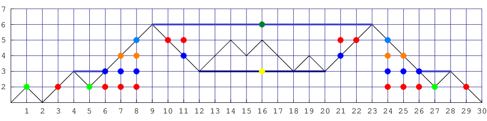
Figure 4: Illustrative example showing three iterative stages of the algorithm for decomposing a particular ALA_{L} path to reveal the particle content and configurations of particles and dual-particles. In the first stage, a new baseline is drawn at height 6. The profile is traced down and to the left and down and to the right. This introduces (upside down) particles of type 1 at positions 5 and 27 and the indicated decorations. In the second stage, a new baseline is drawn at height 3. The profile of the complex between sites 9 and 23 is traced out adding the indicated dual-particle decorations. In the third stage, a new baseline is added at height 5. The profile is traced out and the final decorations added.
Refer to caption
Refer to caption
Refer to caption
Figure 5: A particle of type 11 moving from right to left through a particle of type 33. The configurations as the particle of type 11 progresses further to the left are obtained by reflecting in the vertical. Like solitons, after the interaction, the particles maintain their integrity. On the right, the type 11 and 22 particle and dual-particle content is shown as a string pattern in two strips.
Refer to caption
Refer to caption
Refer to caption
Figure 6: A particle of type 22 moving through a particle of type 33. Like solitons, after the interaction, the particles maintain their integrity. On the right, the type 11 and 22 particle and dual-particle content is shown as a string pattern in two strips.

2.5 Particle content and string patterns

The content of particles and dual particles is conveniently encoded in a pattern of 11- and 22-strings in a number of physical strips as in Figures 5 and 6. The strips can be displayed horizontally or vertically as convenient. Anticipating the connection with lattice models, we call such patterns string patterns or zero patterns. A particle of type aa at position jj corresponds to a 22-string in strip aa at position jj, that is, a pair of zeros at the two edges of the strip with a common coordinate along the strip. A dual-particle of type aa at position jj corresponds to a 11-string in the center of strip aa at position jj. Although the positions jj are used to initially generate the string patterns, only the relative ordering of 11- and 22-strings in each separate strip is relevant. String patterns with the same relative orderings of 11- and 22-strings are regarded as equivalent.

We assert, without proof, that the particle decomposition provides a bijection between RSOS paths and distinct string patterns. The RSOS paths and string patterns are known to give the same finitized characters for arbitrary system size NN. In addition, we have checked this conjecture explicitly for sizes out to N=16N=16 by coding the decomposition algorithm in Mathematica [45]. We hope to give a proper proof of this conjectured bijection elsewhere.

2.6 qq-binomials and particle energies

The distinct string patterns in strip aa with nan_{a} 22-strings and mam_{a} 11-strings are enumerated combinatorially by a qq-binomial generating function [ma+nama]q\mbox{$[{m_{a}+n_{a}\atop m_{a}}]$}_{q} as illustrated in Figure 7. The strip configurations are assigned a weight qEq^{E} and graded by the energy EE. The lowest energy configuration, with all 11-strings above all 22-strings, is assigned the relative energy E=0E=0. Each time a 11-string is pushed down through a 22-string, the energy increases by one unit. This excitation energy is associated with the 1-strings or dual-particles.

→ → → → 1 q ⁢ 2 q 2 q 3 q 4 + + + +
Figure 7: Enumeration, by the qq-binomial [42]q=1+q+2​q2+q3+q4\mbox{$[{4\atop 2}]$}_{q}=1+q+2q^{2}+q^{3}+q^{4}, of distinct string patterns in strip aa with ma=na=2m_{a}=n_{a}=2. For convenience, the strips are displayed vertically with position j=1j=1 at the top.

Integer string quantum numbers

I(a)=(I1(a),I2(a),…,Ima(a))\displaystyle I^{(a)}=(I_{1}^{(a)},I_{2}^{(a)},\ldots,I_{m_{a}}^{(a)}) (2.30)

uniquely label the energy levels of dual-particles in each strip. These are defined by

Ij(a)\displaystyle I_{j}^{(a)} =\displaystyle= {number of 2-strings above the 1-string labelled j in strip a}\displaystyle\left\{\mbox{number of 2-strings above the 1-string labelled $j$ in strip $a$}\right\} (2.31)

Clearly,

na⩾I1(a)⩾I2(a)⩾⋯⩾Ima(a)⩾0\displaystyle n_{a}\geqslant I_{1}^{(a)}\geqslant I_{2}^{(a)}\geqslant\cdots\geqslant I_{m_{a}}^{(a)}\geqslant 0 (2.32)

In addition to the excitation energies described by qq-binomials, there is an energy associated with the creation of the particle content, that is, particles or equivalently dual-particles. In terms of dual-particles, this energy is given by the Cartan matrix. The total energy assigned to a string pattern is

E=−c24+14​𝒎T​C​𝒎+∑a∑jaIja(a)\displaystyle E=-\frac{c}{24}+{1\over 4}\,\mbox{\boldmath$m$}^{T}C\mbox{\boldmath$m$}+\sum_{a}\sum_{j_{a}}I_{j_{a}}^{(a)} (2.33)

where the first term involves the central charge cc given by (1.2) or c=1c=1, the second term is the creation energy of the particles and the third term is the excitation energies arising from the various strips as in Figure 7. The central charge term is added to make contact with finitized characters given by the generating function or configurational sum

χ0(N)​(q)=∑configqE\displaystyle\chi_{0}^{(N)}(q)=\sum_{\rm config}q^{E} (2.34)

where the configurations are enumerated by paths or string patterns. The total energies (2.33) including the central charge term are correctly recovered in the TBA calculations of Sections 3 and 4 based on the string patterns.

2.7 ALA_{L} finitized fermionic characters

In the ALA_{L} case, the generating function for the spectrum of energy (2.33) in the vacuum sector is [6, 7]

χ0,A(N)(q)=q−c/24∑(m,n)q14​𝒎T​C​𝒎∏a=1L−2[ma+nama]q\displaystyle\chi_{0,A}^{(N)}(q)=q^{-c/24}\sum_{(m,n)}q^{{1\over 4}\,\mbox{\scriptsize\boldmath$m$}^{T}C\mbox{\scriptsize\boldmath$m$}}\prod_{a=1}^{L-2}{\Big[{m_{a}+n_{a}\atop m_{a}}\Big]}_{q} (2.35)

where CC is the AL−2A_{L-2} Cartan matrix. This is precisely the finitized vacuum fermionic character of the unitary minimal model ℳ⁡(L,L+1){\cal M}(L,L+1) with central charge cc given by (1.2). In the limit N→∞N\to\infty, with NN even, one obtains the vacuum fermionic character

χ0,A(q)=q−c/24∑ma=0​(mod 2)m1⩾m2⩾…⩾mL−2⩾0q14​𝒎T​C​𝒎(q)m1∏a=2L−2[12​(ma−1+ma+1)ma]q\displaystyle\chi_{0,A}(q)=q^{-c/24}\sum_{m_{a}=0\;\text{(mod 2)}\atop m_{1}\geqslant m_{2}\geqslant\ldots\geqslant m_{L-2}\geqslant 0}{q^{{1\over 4}\,\mbox{\scriptsize\boldmath$m$}^{T}C\mbox{\scriptsize\boldmath$m$}}\over(q)_{m_{1}}}\prod_{a=2}^{L-2}{\Big[{{1\over 2}(m_{a-1}+m_{a+1})\atop m_{a}}\Big]}_{q} (2.36)

where mL−1=0m_{L-1}=0 and the qq-factorial is

(q)m=∏j=1m(1−qj)\displaystyle(q)_{m}=\prod_{j=1}^{m}(1-q^{j}) (2.37)

2.8 TLT_{L} finitized fermionic characters

Combinatorially, in the TLT_{L} case corresponding to the XXX model with central charge c=1c=1, the finitized TLT_{L} vacuum character admits several different forms related to spinons, Young tableaux and rigged configurations. We recall here the finitized [46] and infinite NN forms [47, 48] of this vacuum character.

In the spinon formulation, the finitized TLT_{L} vacuum character admits the fermionic form

χ0,T(N)(q,z)=q−1/24∑Sz=−N/2N/2qSz2z2​Sz[NN/2−Sz]q\chi^{(N)}_{0,T}(q,z)=q^{-1/24}\sum^{N/2}_{S_{z}=-N/2}q^{S_{z}^{2}}z^{2S_{z}}{\Big[{N\atop N/2-S_{z}}\Big]}_{q}

Setting q=z=1q=z=1 gives the counting of states

χ0,T(N)(1,1)=∑Sz=−N/2N/2(NN/2−Sz)= 2N\chi^{(N)}_{0,T}(1,1)\;=\sum^{N/2}_{S_{z}=-N/2}{{N}\choose{N/2-S_{z}}}\;=\;2^{N}

In the XXX spin chain language, N+N_{+}, N−N_{-} and SzS_{z} are quantum numbers. N+N_{+} is the number of up spins and N−N_{-} is the number of down spins so that the number of spins is N=N++N−N=N_{+}+N_{-} and the zz-component of spin is Sz=12​(N+−N−)S_{z}=\mbox{$\textstyle{1\over 2}$}(N_{+}-N_{-}). Defining the quantum-dimension

χn​(z)=zn−z−nz−z−1,n∈ℤ\displaystyle\chi_{n}(z)=\frac{z^{n}-z^{-n}}{z-z^{-1}},\quad n\in\mathbb{Z} (2.38)

there is also a bosonic formula for this character [47]

χ0,T(N)(q,z)=q−1/24∑N+=0⌊N/2⌋χN−2​N++1(z)(q(N/2−N+)2[NN+]q−q(N/2−N++1)2[NN+−1]q)\displaystyle\chi^{(N)}_{0,T}(q,z)=q^{-1/24}\sum^{\lfloor N/2\rfloor}_{N_{+}=0}\chi_{N-2N_{+}+1}(z)\bigg(q^{(N/2-N_{+})^{2}}{\Big[{N\atop N_{+}}\Big]}_{q}-q^{(N/2-N_{+}+1)^{2}}{\Big[{N\atop N_{+}-1}\Big]}_{q}\bigg) (2.39)

As a consequence we have

2N=χ0,T(N)​(1,1)=∑N+=0⌊N/2⌋(N−2​N++1)​Z​(N,N+),Z⁡(N,N+)=(NN+)−(NN+−1)\displaystyle 2^{N}=\chi^{(N)}_{0,T}(1,1)=\sum^{\lfloor N/2\rfloor}_{N_{+}=0}(N-2N_{+}+1)Z(N,N_{+}),\qquad Z(N,N_{+})={{N}\choose{N_{+}}}-{{N}\choose{N_{+}-1}} (2.40)

and N−2​N++1=2​S+1N-2N_{+}+1=2S+1 is the degeneracy of the spin sector with total spin SS.

An alternative fermionic representation of the TLT_{L} vacuum character is given by [47]

χ0,T(N)​(q,z)\displaystyle\chi^{(N)}_{0,T}(q,z) =\displaystyle= q−1/24∑(m,n)χm⌊N/2⌋+1(z)q14​𝒎T​C​𝒎∏a=1⌊N/2⌋[ma+nama]q\displaystyle q^{-1/24}\sum_{(m,n)}\chi_{m_{\lfloor N/2\rfloor}+1}(z)\,q^{{1\over 4}\,\mbox{\scriptsize\boldmath$m$}^{T}C\mbox{\scriptsize\boldmath$m$}}\prod_{a=1}^{\lfloor N/2\rfloor}{\Big[{m_{a}+n_{a}\atop m_{a}}\Big]}_{q} (2.41)

where CC is the TL−1′T_{L-1}^{\prime} Cartan matrix. Let us consider the projection of this character onto the z0z^{0} s​ℓ​(2)s\ell(2) charge sector (Sz=0S_{z}=0)

χ0,T(N)​(q)|z0\displaystyle\chi^{(N)}_{0,T}(q)\Big|_{z^{0}} =\displaystyle= q−1/24∑(m,n)q14​𝒎T​C​𝒎∏a=1⌊N/2⌋[ma+nama]q=q−1/24[NN/2]q\displaystyle q^{-1/24}\sum_{(m,n)}q^{{1\over 4}\,\mbox{\scriptsize\boldmath$m$}^{T}C\mbox{\scriptsize\boldmath$m$}}\prod_{a=1}^{\lfloor N/2\rfloor}{\Big[{m_{a}+n_{a}\atop m_{a}}\Big]}_{q}\;=\;q^{-1/24}{\Big[{N\atop N/2}\Big]}_{q} (2.42)
=\displaystyle= q−1/24∑(m,n)q14​𝒎T​C​𝒎∏a=1K[ma+nama]q\displaystyle q^{-1/24}\sum_{(m,n)}q^{{1\over 4}\,\mbox{\scriptsize\boldmath$m$}^{T}C\mbox{\scriptsize\boldmath$m$}}\prod_{a=1}^{K}{\Big[{m_{a}+n_{a}\atop m_{a}}\Big]}_{q} (2.43)

This is convenient since, from the lattice, this projected character contains all of the distinct eigenvalues (as Laurent polynomials) and removes the degeneracies. In the second formula we have taken an arbitrary integer K>⌊N/2⌋=L−1K>\lfloor N/2\rfloor=L-1 and extended the definitions of 𝒎m and 𝒏n by

na=0,ma=mL−1,a>L−1\displaystyle n_{a}=0,\quad m_{a}=m_{L-1},\qquad a>L-1 (2.44)

with C=TK′C=T^{\prime}_{K}. Taking the limit K→∞K\to\infty followed by N→∞N\to\infty, with NN even, we then obtain the projected vacuum fermionic character

χ0,T(q)|z0=q−1/24∑ma=0​(mod 2)m1⩾m2⩾…⩾0q14​𝒎T​C​𝒎(q)m1∏a=2∞[12​(ma−1+ma+1)ma]q\displaystyle\chi_{0,T}(q)\Big|_{z^{0}}=q^{-1/24}\sum_{m_{a}=0\;\text{(mod 2)}\atop m_{1}\geqslant m_{2}\geqslant\ldots\geqslant 0}{q^{{1\over 4}\,\mbox{\scriptsize\boldmath$m$}^{T}C\mbox{\scriptsize\boldmath$m$}}\over(q)_{m_{1}}}\prod_{a=2}^{\infty}{\Big[{{1\over 2}(m_{a-1}+m_{a+1})\atop m_{a}}\Big]}_{q} (2.45)

where CC is now the Cartan matrix of T∞′=A∞T^{\prime}_{\infty}=A_{\infty} and the sum is over asymptotically constant configurations 𝒎m for which there exists some finite K>0K>0 such that ma=mKm_{a}=m_{K} whenever a>Ka>K.

2.9 One-dimensional configurational sums

Typically, finitized characters can be expressed as one-dimensional configurational sums, that is, via an energy statistic applied directly to RSOS paths. These one-dimensional configurational sums first appeared in the work of Baxter [3] but in the context of off-critical Corner Transfer Matrices (CTMs) where the elliptic nome q^\hat{q} (1.3) is related to the departure from criticality. By contrast, we work here only at criticality and qq is always the modular nome.

The one-dimensional configurational sums are defined by

Xa​b​c(N)​(q)=∑{σ}q12​∑j=1Nj​H​(σj−1,σj,σj+1),σ0=a,σN=b,σN+1=cX^{(N)}_{abc}(q)=\sum_{\{\sigma\}}q^{{1\over 2}\sum_{j=1}^{N}jH(\sigma_{j-1},\sigma_{j},\sigma_{j+1})},\qquad\sigma_{0}=a,\ \ \sigma_{N}=b,\ \ \sigma_{N+1}=c (2.46)

where H⁡(σj−1,σj,σj+1)H(\sigma_{j-1},\sigma_{j},\sigma_{j+1}) is a local energy (energy density) and the sum is over all RSOS paths σ={σ0,σ1,…,σN+1}\sigma=\{\sigma_{0},\sigma_{1},\ldots,\sigma_{N+1}\} on ALA_{L} or TLT_{L} with σj∈{1,2,…,L}\sigma_{j}\in\{1,2,\ldots,L\}. These one-dimensional configurational sums satisfy mathematically powerful recursion relations in NN relating different boundary conditions specified by a,ba,b and cc. In the vacuum sector with NN even, a=b=1a=b=1 and c=2c=2.

The form of the local energy function is not uniquely determined due to the possibility of local gauge transformations. Let us choose, however, the local energy function to be of the simple form

H⁡(σj−1,σj,σj+1)={1,(σj−1,σj,σj+1)=(1,1,1)12,(σj−1,σj,σj+1)=(1,1,2)​or​(2,1,1)1,|σj−1−σj+1|=20,otherwise\displaystyle H(\sigma_{j-1},\sigma_{j},\sigma_{j+1})=\begin{cases}1,&(\sigma_{j-1},\sigma_{j},\sigma_{j+1})=(1,1,1)\\ \mbox{$\textstyle{1\over 2}$},&(\sigma_{j-1},\sigma_{j},\sigma_{j+1})=(1,1,2)\ \mbox{or}\ (2,1,1)\\ 1,&|\sigma_{j-1}-\sigma_{j+1}|=2\\ 0,&\mbox{otherwise}\end{cases} (2.47)

It is then confirmed that, for both ALA_{L} and TLT_{L} paths, the energy statistic

E=−c24+12​∑j=1Nj​H​(σj−1,σj,σj+1)\displaystyle E=-{c\over 24}+{1\over 2}\sum_{j=1}^{N}j\,H(\sigma_{j-1},\sigma_{j},\sigma_{j+1}) (2.48)

exactly reproduces the string energies (2.33) and hence

χ0,A(N)(q)=q−c/24X112(N)(q)\displaystyle\chi_{0,A}^{(N)}(q)=q^{-c/24}X_{112}^{(N)}(q) (2.49)

This relation has been checked directly in Mathematica [45] for all sizes up to to N=26N=26 and confirms the equivalence of (2.33) and (2.48). This largest size involves 10.6 million paths.

2.10 Combinatorial classification of states

The combinatorial classification of states for the A5A_{5} minimal model for paths of length N=8N=8 is shown in Figures 8 and 9. In this case there are 14 such states with the finitized vacuum character

χ0,A5(8)(q)=q−1/30(1+q2+q3+2q4+q5+2q6+q7+2q8+q9+q10+q12)\displaystyle\chi_{0,A_{5}}^{(8)}(q)=q^{-1/30}(1+q^{2}+q^{3}+2q^{4}+q^{5}+2q^{6}+q^{7}+2q^{8}+q^{9}+q^{10}+q^{12}) (2.50)

The combinatorial classification of states for the T5T_{5} XXX model for paths of length N=6N=6 is shown in Figures 10 through 12. In this case there are 20 such states with the finitized vacuum character

χ0,T(6)(q)=q−1/24(1+q+2q2+3q3+3q4+3q5+3q6+2q7+q8+q9)\displaystyle\chi_{0,T}^{(6)}(q)=q^{-1/24}(1+q+2q^{2}+3q^{3}+3q^{4}+3q^{5}+3q^{6}+2q^{7}+q^{8}+q^{9}) (2.51)

In both of these cases, there are 3 physical strips and we see that the patterns of 1-strings and 2-strings in these strips arising from the particle decompositions of the paths exactly match the patterns of eigenvalue zeros in the upper-half uu-plane obtained by direct diagonalization of the commuting double row transfer matrices with NN faces along a row.

The particular system sizes in these examples were chosen for convenience in illustrating the combinatorial classification of states. Many values for LL and NN have been checked, in particular considerably larger system sizes, and in all cases perfect agreement was found between the combinatorial picture in terms of paths and the numerical location of zeros of eigenvalues of the transfer matrices.

1. E=0E=0:  Refer to captionRefer to caption
2. E=2E=2:  Refer to captionRefer to caption
3. E=3E=3:  Refer to captionRefer to caption
4. E=4E=4:  Refer to captionRefer to caption
5. E=4E=4:  Refer to captionRefer to caption
6. E=5E=5:  Refer to captionRefer to caption
7. E=6E=6:  Refer to captionRefer to caption
Figure 8: Eigenvalues 1 to 7 for A5A_{5} with N=8N=8 showing the energies (omitting the −c/24-c/24 term), paths, predicted patterns of zeros and actual patterns of zeros (rotated through 90 degrees) from numerical diagonalization of transfer matrices. Only the relative order of 1- and 2-strings in each strip is relevant. The relative order across strips is not relevant.

8. E=6E=6:  Refer to captionRefer to caption
9. E=7E=7:  Refer to captionRefer to caption
10. E=8E=8:  Refer to captionRefer to caption
11. E=8E=8:  Refer to captionRefer to caption
12. E=9E=9:  Refer to captionRefer to caption
13. E=10E=10:  Refer to captionRefer to caption
14. E=12E=12:  Refer to captionRefer to caption
Figure 9: This is a continuation of Figure 8 showing eigenvalues 8 to 14 for A5A_{5} with N=8N=8.

1. E=0E=0  Refer to caption   Refer to caption
2. E=1E=1  Refer to caption   Refer to caption
3. E=2E=2  Refer to caption   Refer to caption
4. E=2E=2  Refer to caption   Refer to caption
5. E=3E=3  Refer to caption   Refer to caption
6. E=3E=3  Refer to caption   Refer to caption
7. E=3E=3  Refer to caption   Refer to caption
Figure 10: Eigenvalues 1 to 7 for the XXX model with N=6N=6 showing the energies (omitting the −c/24-c/24 term), paths and actual patterns of zeros (rotated through 90 degrees) from numerical diagonalization of transfer matrices. Only the relative order of 1- and 2-strings in each strip is relevant. The last column shows the numerical patterns of zeros for the eigenvalues of the auxiliary matrix QQ. The QQ eigenvalue has a jj-string at the same relative position for each 2-string in strip jj of the transfer matrix eigenvalues. The path out to j=7j=7 is needed to apply (2.33).

8. E=4E=4  Refer to caption   Refer to caption
9. E=4E=4  Refer to caption   Refer to caption
10. E=4E=4  Refer to caption   Refer to caption
11. E=5E=5  Refer to caption   Refer to caption
12. E=5E=5  Refer to caption   Refer to caption
13. E=5E=5  Refer to caption   Refer to caption
14. E=6E=6  Refer to caption   Refer to caption
Figure 11: This is a continuation of Figure 10 showing eigenvalues 8 to 14 for the XXX model with N=6N=6.

15. E=6E=6  Refer to caption   Refer to caption
16. E=6E=6  Refer to caption   Refer to caption
17. E=7E=7  Refer to caption   Refer to caption
18. E=7E=7  Refer to caption   Refer to caption
19. E=8E=8  Refer to caption   Refer to caption
20. E=9E=9  Refer to caption   Refer to caption
Figure 12: This is a continuation of Figures 10 and 11 showing eigenvalues 15 to 20 for the XXX model with N=6N=6.

2.11 Bethe roots and transfer matrix 2-strings for XXX model

In Figures 10 through 12, relevant to the XXX model, we have also shown the eigenvalue zeros of Baxter’s auxiliary matrix 𝑸⁡(u)\mbox{\boldmath$Q$}(u) as in (4.3) and (4.4). These zeros are precisely the Bethe ansatz roots. The transfer matrices 𝑫q​(u)\mbox{\boldmath$D$}^{q}(u) are completely determined by knowledge of the matrix 𝑸⁡(u)\mbox{\boldmath$Q$}(u) through Baxter’s TT-QQ relation (4.3) and the fusion hierarchy.

It is readily confirmed, in this example, that an eigenvalue Q⁡(u)Q(u) has a jj-string at the same relative position as each 2-string in strip jj of the transfer matrix eigenvalues with j=1,2,…,N/2j=1,2,\ldots,N/2. Identifying S=n0/2S=n_{0}/2 as the total spin, we see that there are 5,9,5,15,9,5,1 eigenvalues with total spin S=0,1,2,3S=0,1,2,3 respectively in the Sz=0S_{z}=0 sector. The zero content of an eigenvalue Q⁡(u)Q(u) thus determines the complete particle content nan_{a} with a=0,1,…,N/2−1a=0,1,\ldots,N/2-1. The dual-particle content then follows from the (m,n)(m,n) system (2.25). Again we have verified these observations for many different system sizes NN. We further conjecture that these observations hold true for all NN and that in the limit N→∞N\to\infty the locations of the jj-strings of Q⁡(u)Q(u) exactly coincide with the locations of the 2-strings of the transfer matrices in strip jj.

3 Unitary Minimal RSOS Lattice Models

The bulk face and boundary triangle Boltzmann weights of the critical unitary minimal RSOS models [28, 35] on ALA_{L} in the vacuum sector are

-1,-1)(6,6) ).35090 =s(λ−u)δa,c+s(u)Sa​ScSb​Sdδb,d,-1,-1)(4,6) =-1,-1)(4,6) =S2δa,1δb,2\begin{pspicture}shift=-2.4[(]-1,-1)(6,6) ){.35}{0}{90} \end{pspicture}\;=\;s(\lambda-u)\,\delta_{a,c}+s(u)\sqrt{S_{a}S_{c}\over S_{b}S_{d}}\,\delta_{b,d},\qquad\qquad\begin{pspicture}shift=-2.4[(]-1,-1)(4,6) \end{pspicture}\;=\;\begin{pspicture}shift=-2.4[(]-1,-1)(4,6) \end{pspicture}\;=\;\sqrt{S_{2}}\,\delta_{a,1}\delta_{b,2} (3.1)

where

s⁡(u)=sin⁡usin⁡λ=z−z−1x−x−1,z=ei​u,x=ei​λ,λ=πL+1,Sa=s⁡(a​λ)\displaystyle s(u)={\sin u\over\sin\lambda}={z-z^{-1}\over x-x^{-1}},\quad z=e^{iu},\quad x=e^{i\lambda},\quad\lambda={\pi\over L+1},\quad S_{a}=s(a\lambda) (3.2)

Commuting double row transfer matrices can now be defined following [35].

3.1 Bethe ansatz

The double row transfer matrices of the unitary minimal models in the vacuum sector satisfy the TT-QQ functional equation [10] modified to account for the boundary

s⁡(2​u)​𝑫​(u+λ2)​𝑸​(u)=s⁡(2​u+λ)​f​(u+λ2)​𝑸​(u−λ)+s⁡(2​u−λ)​f​(u−λ2)​𝑸​(u+λ)\displaystyle s(2u)\,\mbox{\boldmath$D$}(u+{\lambda\over 2})\mbox{\boldmath$Q$}(u)=s(2u+\lambda)f(u+{\lambda\over 2})\mbox{\boldmath$Q$}(u-\lambda)+s(2u-\lambda)f(u-{\lambda\over 2})\mbox{\boldmath$Q$}(u+\lambda) (3.3)

where f⁡(u)=s​(u)2​Nf(u)=s(u)^{2N} and 𝑸⁡(u)\mbox{\boldmath$Q$}(u) is an auxiliary family of matrices satisfying [𝑸⁡(u),𝑸⁡(v)]=[𝑸⁡(u),𝑫⁡(v)]=𝟎[\mbox{\boldmath$Q$}(u),\mbox{\boldmath$Q$}(v)]=[\mbox{\boldmath$Q$}(u),\mbox{\boldmath$D$}(v)]=\mbox{\boldmath$0$}. The same functional equation is satisfied by the eigenvalues D⁡(u)D(u) and Q⁡(u)Q(u) and so the Bethe ansatz equations result by setting

Q⁡(u)=∏j=1ns⁡(u−uj)​s​(u+uj)\displaystyle Q(u)=\prod_{j=1}^{n}s(u-u_{j})s(u+u_{j}) (3.4)

where uju_{j} are the r=2​nr=2n Bethe roots. The physical analyticity strip of D⁡(u)D(u) is −λ/2<Reu<3λ/2-\lambda/2<\mathop{\rm Re}u<3\lambda/2 and the physical analyticity strip of D~​(u)=D​(u+λ2)\tilde{D}(u)=D(u+{\lambda\over 2}) is −λ<Reu<λ-\lambda<\mathop{\rm Re}u<\lambda.

Let 𝑫⁡(u)=𝑫01\mbox{\boldmath$D$}(u)=\mbox{\boldmath$D$}_{0}^{1} and

𝑫kq=𝑫q​(u+k​λ),𝑸k=𝑸⁡(u+k​λ),sk​(u)=s⁡(2​u+k​λ),fk​(u)=(−1)N​s​(u+k​λ)2​N\displaystyle\mbox{\boldmath$D$}_{k}^{q}=\mbox{\boldmath$D$}^{q}(u+k\lambda),\quad\mbox{\boldmath$Q$}_{k}=\mbox{\boldmath$Q$}(u+k\lambda),\quad s_{k}(u)={s(2u+k\lambda)},\quad f_{k}(u)=(-1)^{N}{s(u+k\lambda)}^{2N} (3.5)

then the TT-QQ relation implies that the eigenvalues D⁡(u)D(u) are determined by the eigenvalues Q⁡(u)Q(u) in the compact form

D~0=s1f1/2Q−1+s−1f−1/2Q1s0​Q0\displaystyle\tilde{D}_{0}={s_{1}f_{1/2}Q_{-1}+s_{-1}f_{-1/2}Q_{1}\over s_{0}Q_{0}} (3.6)

3.2 Functional equations

The fused transfer matrices 𝑫q\mbox{\boldmath$D$}^{q} satisfy the fusion hierarchy of functional equations [30, 35]

sq−2s2​q−1𝑫0q𝑫q1=sq−3s2​qfq𝑫0q−1+sq−1s2​q−2fq−1𝑫0q+1,q=1,2,…,L−1\displaystyle s_{q-2}s_{2q-1}\mbox{\boldmath$D$}_{0}^{q}\mbox{\boldmath$D$}_{q}^{1}=s_{q-3}s_{2q}f_{q}\mbox{\boldmath$D$}_{0}^{q-1}+s_{q-1}s_{2q-2}f_{q-1}\mbox{\boldmath$D$}_{0}^{q+1},\qquad q=1,2,\ldots,L-1 (3.7)

subject to the closure conditions

𝑫0−1=0,𝑫00=f−1​𝑰,𝑫0L=0\displaystyle\mbox{\boldmath$D$}_{0}^{-1}=0,\qquad\mbox{\boldmath$D$}_{0}^{0}=f_{-1}\mbox{\boldmath$I$},\qquad\mbox{\boldmath$D$}_{0}^{L}=0 (3.8)

Starting with the fusion hierarchy, induction can be used to derive the TT-system of functional equations [32, 35]

sq−2sq𝑫0q𝑫1q=s−2s2​qf−1fq𝑰+sq−12𝑫0q+1𝑫1q−1,q=1,2,…,L−1\displaystyle s_{q-2}s_{q}\mbox{\boldmath$D$}_{0}^{q}\mbox{\boldmath$D$}_{1}^{q}=s_{-2}s_{2q}f_{-1}f_{q}\mbox{\boldmath$I$}+s_{q-1}^{2}\mbox{\boldmath$D$}_{0}^{q+1}\mbox{\boldmath$D$}_{1}^{q-1},\qquad q=1,2,\ldots,L-1 (3.9)

For q=1q=1, this is just the usual inversion identity given by the fusion hierarchy with q=1q=1.

If we further define

𝒅0q=sq−12​𝑫1q−1​𝑫0q+1s−2​s2​q​f−1​fq,q=1,2,…,L−2\displaystyle\mbox{\boldmath$d$}_{0}^{q}={s_{q-1}^{2}\mbox{\boldmath$D$}_{1}^{q-1}\mbox{\boldmath$D$}_{0}^{q+1}\over s_{-2}s_{2q}f_{-1}f_{q}},\qquad q=1,2,\ldots,L-2 (3.10)

then the inversion identity hierarchy can be recast in the form of the YY-system [32, 35]

𝒅0q​𝒅1q\displaystyle\mbox{\boldmath$d$}_{0}^{q}\mbox{\boldmath$d$}_{1}^{q} =\displaystyle= sq−12​sq+12​(𝑫0q+1​𝑫1q+1)​(𝑫1q−1​𝑫2q−1)s−2​s0​s2​q​s2​q+2​f−1​f0​fq​fq+1\displaystyle{s_{q-1}^{2}s_{q+1}^{2}(\mbox{\boldmath$D$}_{0}^{q+1}\mbox{\boldmath$D$}_{1}^{q+1})(\mbox{\boldmath$D$}_{1}^{q-1}\mbox{\boldmath$D$}_{2}^{q-1})\over s_{-2}s_{0}s_{2q}s_{2q+2}f_{-1}f_{0}f_{q}f_{q+1}} (3.11)
=\displaystyle= (𝑰+sq2​𝑫0q+2​𝑫1qs−2​s2​q+2​f−1​fq+1)​(𝑰+sq2​𝑫1q​𝑫2q−2s0​s2​q​f0​fq)=(𝑰+𝒅0q+1)​(𝑰+𝒅1q−1)\displaystyle\Big(\mbox{\boldmath$I$}+{s_{q}^{2}\mbox{\boldmath$D$}_{0}^{q+2}\mbox{\boldmath$D$}_{1}^{q}\over s_{-2}s_{2q+2}f_{-1}f_{q+1}}\Big)\!\!\Big(\mbox{\boldmath$I$}+{s_{q}^{2}\mbox{\boldmath$D$}_{1}^{q}\mbox{\boldmath$D$}_{2}^{q-2}\over s_{0}s_{2q}f_{0}f_{q}}\Big)\;=\;\big(\mbox{\boldmath$I$}+\mbox{\boldmath$d$}_{0}^{q+1}\big)\big(\mbox{\boldmath$I$}+\mbox{\boldmath$d$}_{1}^{q-1}\big)

with closure

𝒅00=𝒅0L−1=0\displaystyle\mbox{\boldmath$d$}_{0}^{0}=\mbox{\boldmath$d$}_{0}^{L-1}=0 (3.12)

We wish to solve the YY-system (3.11) subject to the constraints of periodicity, conjugation and crossing symmetries, analyticity and asymptotic limits. The periodicity, conjugation and crossing symmetries are

𝑫q​(u)=𝑫q​(u+π),𝑫q​(u)=𝑫q​(λ−u)\displaystyle\mbox{\boldmath$D$}^{q}(u)=\mbox{\boldmath$D$}^{q}(u+\pi),\qquad\mbox{\boldmath$D$}^{q}(u)=\mbox{\boldmath$D$}^{q}(\lambda-u) (3.13)
Dq​(u)¯=Dq​(u)=Dq​((2−q)​λ−u),dq​(u)¯=dq​(u)=dq​((1−q)​λ−u)\displaystyle\overline{D^{q}(u)}=D^{q}(u)=D^{q}\big((2-q)\lambda-u\big),\qquad\overline{d^{q}(u)}=d^{q}(u)=d^{q}\big((1-q)\lambda-u\big) (3.14)

To discuss analyticity, we consider the eigenvalues of the transfer matrices 𝑫q​(u)\mbox{\boldmath$D$}^{q}(u) and 𝒅q​(u)\mbox{\boldmath$d$}^{q}(u) at each fusion level in their respective analyticity strips

−q2​λ<Reu<4−q2​λ,−q+12​λ<Reu<3−q2​λ\displaystyle-{q\over 2}\,\lambda<\mathop{\rm Re}u<{4-q\over 2}\,\lambda,\qquad-{q+1\over 2}\,\lambda<\mathop{\rm Re}u<{3-q\over 2}\,\lambda (3.15)

Defining the shifted transfer matrices

𝑫~q​(u)=𝑫q​(u+2−q2​λ),𝒅~q​(u)=𝒅q​(u+1−q2​λ)\tilde{\mbox{\boldmath$D$}}^{q}(u)=\mbox{\boldmath$D$}^{q}\Big(u+{2-q\over 2}\,\lambda\Big),\qquad\tilde{\mbox{\boldmath$d$}}^{q}(u)=\mbox{\boldmath$d$}^{q}\Big(u+{1-q\over 2}\,\lambda\Big) (3.16)

it follows that these transfer matrices have the common analyticity strip

−λ<Re(u)<λ\displaystyle-\lambda<\mathop{\rm Re}(u)<\lambda (3.17)

and satisfy the same periodicity (3.13) with crossing symmetries

D~q​(u)=D~q​(−u),d~q​(u)=d~q​(−u)\tilde{D}^{q}(u)=\tilde{D}^{q}(-u),\qquad\tilde{d}^{q}(u)=\tilde{d}^{q}(-u) (3.18)

In terms of shifted transfer matrices, the TBA functional equations take the form

𝒅~q​(u−λ2)​𝒅~q​(u+λ2)=(1+𝒅~q−1​(u))​(1+𝒅~q+1​(u))\displaystyle\tilde{\mbox{\boldmath$d$}}^{q}\big(u-\frac{\lambda}{2}\big)\ \tilde{\mbox{\boldmath$d$}}^{q}\big(u+\frac{\lambda}{2}\big)=\big(1+\tilde{\mbox{\boldmath$d$}}^{q-1}(u)\big)\big(1+\tilde{\mbox{\boldmath$d$}}^{q+1}(u)\big) (3.19)

Lastly, the asymptotic values dj​(+i​∞)d^{j}(+i\infty) were computed in [32]

d~j​(+i​∞)\displaystyle\tilde{d}^{j}(+i\infty) =\displaystyle= sin⁡[j​θ]​sin⁡[(j+2)​θ]sin2⁡θ=sin2⁡(j+1)​θsin2⁡θ−1,θ=s​πL+1\displaystyle\frac{\sin[j\theta]\>\sin[(j+2)\theta]}{\sin^{2}\theta}\;=\;\frac{\sin^{2}(j+1)\theta}{\sin^{2}\theta}-1,\qquad\theta=\frac{s\pi}{L+1} (3.20)

Here, ss is a Kac label and plays the role of selecting the eigenstates of the transfer matrix that, in the scaling limit, will be in the (r,s)(r,s) sector of the conformal field theory. More precisely, ss is a good quantum number for the finite system corresponding to the braid limit u→i​∞u\rightarrow i\infty. In contrast, rr is only a good quantum number in the limit N→∞N\to\infty and so is not accessible directly on a finite lattice (see after (3.94)). In the vacuum sector of interest here, (r,s)=(1,1)(r,s)=(1,1).

3.3 Analyticity and solution of TBA

We use analyticity properties of the transfer matrices to transform the YY-system (3.11) into the form of Thermodynamic Bethe Ansatz (TBA) equations. For the ALA_{L} lattice model, these TBA equations take the form of coupled integral equations whose structure is governed by the Dynkin diagram G∗=AL−2G^{*}=A_{L-2}. The analyticity is encoded in the relative locations of the 1- and 2-strings in the analyticity strips (3.15). The TBA equations can be completely solved in the scaling limit for the locations of the 1-strings as well as the excitation energies. Following [37], the strategy is as follows:

  1. 1.

    The special case q=1q=1 of (3.9) provides the expression for the energies or, equivalently, the eigenvalues of the transfer matrix. This expression contains an unknown function (pseudoenergy in the first strip) and a number of unknown real numbers (location of 1-strings in the first strip).

  2. 2.

    The Y-system (3.11) can be transformed into the set of TBA equations.

  3. 3.

    The Y-system (3.11) allows us to access the location of the 1-strings by a set of coupled auxiliary equations, that perform the job of quantisation conditions.

  4. 4.

    The simultaneous solution of TBA plus auxiliary equations completely fixes the pseudoenergies, the locations of the 1-strings and the energy expression.

3.3.1 Analyticity: the energy

We aim at finding the transfer matrix eigenvalues in the physical strip λ2<Reu<3​λ2\frac{\lambda}{2}<\mathop{\rm Re}u<\frac{3\lambda}{2}. We start from the case q=1q=1 of (3.9), written for the eigenvalues of the corresponding matrices

(sin⁡2​λsin⁡λ)2​s−1​s1s−2​s2​f−1​f1​D1​(u)​D1​(u+λ)=1+d1​(u)\left(\frac{\sin 2\lambda}{\sin\lambda}\right)^{2}\frac{s_{-1}s_{1}}{s_{-2}s_{2}\ f_{-1}f_{1}}~D^{1}(u)\ D^{1}(u+\lambda)=1+d^{1}(u) (3.21)

Ignoring the term d1​(u)d^{1}(u) which is exponentially small for large NN, this functional equation factorizes into bulk and boundary equations with D1​(u)=κbulk​(u)​κ0​(u)D^{1}(u)=\kappa_{\text{bulk}}(u)\kappa_{0}(u)

[κbulk​(u)​κbulk​(u+λ)]2​N=f−1​f1=[sin⁡(λ−u)​sin⁡(λ+u)sin2⁡λ]2​N,Reu∈(−λ2,λ2)[\kappa_{\text{bulk}}(u)\ \kappa_{\text{bulk}}(u+\lambda)]^{2N}=f_{-1}f_{1}=\left[\frac{\sin(\lambda-u)\sin(\lambda+u)}{\sin^{2}\lambda}\right]^{2N},\qquad\mathop{\rm Re}u\in(-\frac{\lambda}{2},\frac{\lambda}{2}) (3.22)
κ0​(u)​κ0​(u+λ)=s−2​s2s−1​s1​(sin⁡λsin⁡2​λ)2=sin⁡(λ−2​u)​sin⁡(λ+2​u)sin⁡(2​λ−2​u)​sin⁡(2​λ+2​u)​(sin⁡λsin⁡2​λ)2,Reu∈(−λ2,λ2)\kappa_{0}(u)\ \kappa_{0}(u+\lambda)=\frac{s_{-2}s_{2}}{s_{-1}s_{1}}\left(\frac{\sin\lambda}{\sin 2\lambda}\right)^{2}=\frac{\sin(\lambda-2u)\sin(\lambda+2u)}{\sin(2\lambda-2u)\sin(2\lambda+2u)}\left(\frac{\sin\lambda}{\sin 2\lambda}\right)^{2},\quad\mathop{\rm Re}u\in(-\frac{\lambda}{2},\frac{\lambda}{2}) (3.23)

The expressions for these factors are given in [49] and immediately extend to the whole physical strip Reu∈(−λ2,32​λ)\mathop{\rm Re}u\in(-\frac{\lambda}{2},\frac{3}{2}\lambda). It follows that the “finite” part of the transfer matrix is defined

Dfinite1​(u)=D1​(u)[κbulk​(u)]2​N​κ0​(u)=D~finite1​(u−λ2),Reu∈(−λ2,32​λ).D_{\text{finite}}^{1}(u)=\frac{D^{1}(u)}{[\kappa_{\text{bulk}}(u)]^{2N}\ \kappa_{0}(u)}=\tilde{D}_{\text{finite}}^{1}(u-\frac{\lambda}{2})\,,\qquad\mathop{\rm Re}u\in(-\frac{\lambda}{2},\frac{3}{2}\lambda)\,. (3.24)

Here we do not make use of these factors we only need to know that, from [49], they do not introduce new zeros or poles to Dfinite1​(u)D_{\text{finite}}^{1}(u) in the physical strip. It follows that the finite transfer matrix has precisely the same zeros as D1​(u)D^{1}(u) and no poles. The functional equation (3.21) now takes the form

D~finite1​(u−λ2)​D~finite1​(u+λ2)=1+d1​(u),Reu∈(−λ2,λ2).\tilde{D}^{1}_{\text{finite}}(u-\frac{\lambda}{2})\ \tilde{D}_{\text{finite}}^{1}(u+\frac{\lambda}{2})=1+d^{1}(u)\,,\qquad\mathop{\rm Re}u\in(-\frac{\lambda}{2},\frac{\lambda}{2})\,. (3.25)

Let yk(1)y_{k}^{(1)} denote the location of the zeros of D~1​(u)\tilde{D}^{1}(u) such that

D~finite1​(±i​λπ​yk(1))=D~1​(±i​λπ​yk(1))=0,yk(1)>0.\tilde{D}_{\text{finite}}^{1}(\pm\frac{i\lambda}{\pi}y_{k}^{(1)})=\tilde{D}^{1}(\pm\frac{i\lambda}{\pi}y_{k}^{(1)})=0\,,\qquad y_{k}^{(1)}>0\,. (3.26)

To remove these zeros from D~1​(u)\tilde{D}^{1}(u), we construct the function

Z⁡(u)=∏k=1m1[tanh⁡yk(1)+i⁡(L+1)​u2​tanh⁡yk(1)−i⁡(L+1)​u2],Reu∈(−λ,λ)Z(u)=\prod_{k=1}^{m_{1}}\left[\tanh\frac{y_{k}^{(1)}+i(L+1)u}{2}\ \tanh\frac{y_{k}^{(1)}-i(L+1)u}{2}\right]\,,\qquad\mathop{\rm Re}u\in(-\lambda,\lambda) (3.27)

In the indicated region this function has the same zeros as D~1​(u)\tilde{D}^{1}(u) and no other zeros or poles. Moreover, it satisfies the inversion identity

Z⁡(u−λ2)​Z​(u+λ2)=1.Z(u-\frac{\lambda}{2})Z(u+\frac{\lambda}{2})=1\,. (3.28)

Let us define the function

𝒜⁡(x)=D~finite1​(u)Z⁡(u)|u=i​xL+1,Reu∈(−λ,λ)\mathcal{A}(x)=\frac{\tilde{D}^{1}_{\text{finite}}(u)}{Z(u)}\Big|_{u=\frac{ix}{L+1}}\,,\qquad\mathop{\rm Re}u\in(-\lambda,\lambda) (3.29)

which is free of zeros and poles in the analyticity strip Im​x∈(−π,π)\mbox{Im}x\in(-\pi,\pi). Dividing (3.25) by (3.28) we then obtain

𝒜⁡(x+i​π2)​𝒜​(x−i​π2)=1+ε~1​(x),Im​x∈(−π2,π2)\mathcal{A}(x+\frac{i\pi}{2})\,\mathcal{A}(x-\frac{i\pi}{2})=1+{\tilde{\varepsilon}}^{1}(x)\,,\qquad\mbox{Im}\,x\in(-\frac{\pi}{2},\frac{\pi}{2}) (3.30)

where

ε~q​(x)=d~q​(u)|u=i​xL+1.{\tilde{\varepsilon}}^{q}(x)=\tilde{d}^{q}(u)\big|_{u=\frac{ix}{L+1}}\,. (3.31)

The left side of (3.30) is free of zeros and poles in the indicated region so the right side never vanishes. The function d~1​(u)\tilde{d}^{1}(u) vanishes at u=0u=0 by (3.10) and (3.8). We conclude that

1+ε~1​(x)>0forx∈ℝ1+{\tilde{\varepsilon}}^{1}(x)>0\quad\mbox{for}\quad x\in\mathbb{R} (3.32)

so that we can take the logarithmic derivative

dd​x​log⁡𝒜⁡(x+i​π2)+dd​x​log⁡𝒜⁡(x−i​π2)=dd​x​log⁡(1+ε~1​(x))\frac{d}{dx}\log\mathcal{A}(x+\frac{i\pi}{2})+\frac{d}{dx}\log\mathcal{A}(x-\frac{i\pi}{2})=\frac{d}{dx}\log(1+{\tilde{\varepsilon}}^{1}(x)) (3.33)

Taking Fourier transforms

ℱ⁡(f,k)=12​π​∫−∞∞d​x​f​(x)​e−i​k​x,f⁡(x)=∫−∞∞d​k​ℱ​(f,k)​ei​k​x\displaystyle\mathcal{F}(f,k)=\frac{1}{2\pi}\int_{-\infty}^{\infty}dx\,f(x)\,e^{-ikx},\qquad f(x)=\int_{-\infty}^{\infty}dk\,\mathcal{F}(f,k)\,e^{ikx} (3.34)

we obtain

ℱ⁡(dd​x​log⁡𝒜⁡(x),k)​ 2​cosh⁡(k​π2)=ℱ⁡(dd​x​log⁡(1+ε~1​(x)),k)\mathcal{F}\Big(\frac{d}{dx}\log\mathcal{A}(x),k\Big)\ 2\cosh(k\frac{\pi}{2})=\mathcal{F}\Big(\frac{d}{dx}\log(1+{\tilde{\varepsilon}}^{1}(x)),k\Big) (3.35)

Transforming back, we obtain a convolution with a kernel and an integration constant

log⁡𝒜⁡(x)=∫−∞∞d​y​log⁡(1+ε~1​(y))2​π​cosh⁡(x−y)+const=(K∗log⁡(1+ε~1))​(x)+const\log\mathcal{A}(x)=\int_{-\infty}^{\infty}dy\ \frac{\log(1+{\tilde{\varepsilon}}^{1}(y))}{2\pi\cosh(x-y)}+\mbox{const}=\big(K*\log(1+{\tilde{\varepsilon}}^{1})\big)(x)+\mbox{const} (3.36)

where

(f∗g)​(x)=12​π​∫−∞∞d​y​f​(x−y)​g​(y),K⁡(x)=1cosh⁡x.\displaystyle(f*g)(x)=\frac{1}{2\pi}\int_{-\infty}^{\infty}dy\>f(x-y)\,g(y),\qquad K(x)=\frac{1}{\cosh x}\,. (3.37)

Using (3.24), (3.29) and the needed functions we can reconstruct the initial double row transfer matrix eigenvalues log⁡D1​(λ2+i​xL+1)\log D^{1}(\frac{\lambda}{2}+\frac{ix}{L+1}). Actually, here we are concerned with the finite size corrections to it namely those terms that characterise the scaling limit of the theory. These terms behave as 1/N1/N in the log of the transfer matrix. The bulk term in (3.24) is of order NN; the boundary one and the integration constant are of order 1 and will be ignored. What remains expresses the scaling part of the free energy (in (3.36) we ignored the constant)

fscal.​(x)=−log⁡Dfinite1​(λ2+i​xL+1)=−log⁡𝒜⁡(x)−Z⁡(i​xL+1)=\displaystyle f_{\text{scal.}}(x)=-\log D^{1}_{\text{finite}}(\frac{\lambda}{2}+\frac{ix}{L+1})=-\log\mathcal{A}(x)-Z(\frac{ix}{L+1})= (3.38)
−(K∗log⁡(1+ε~1))​(x)−∑k=1m1[log⁡tanh⁡yk(1)−x2+log⁡tanh⁡yk(1)+x2]\displaystyle-\big(K*\log(1+{\tilde{\varepsilon}}^{1})\big)(x)-\sum_{k=1}^{m_{1}}\left[\log\tanh\frac{y_{k}^{(1)}-x}{2}+\log\tanh\frac{y_{k}^{(1)}+x}{2}\right]

We can fix x=0x=0 namely choose the isotropic point of the system and get

fscal.=−logDfinite1(λ2)=−∫−∞∞dylog⁡(1+ε~1​(y))2​π​cosh⁡(y)−2∑k=1m1logtanhyk(1)2\displaystyle f_{\text{scal.}}=-\log D^{1}_{\text{finite}}(\frac{\lambda}{2})=-\int_{-\infty}^{\infty}dy\ \frac{\log(1+{\tilde{\varepsilon}}^{1}(y))}{2\pi\cosh(y)}-2\sum_{k=1}^{m_{1}}\log\tanh\frac{y_{k}^{(1)}}{2} (3.39)
=2​πN​E+higher order corrections in ​1N\displaystyle=\frac{2\pi}{N}E+\text{higher order corrections in }\frac{1}{N}

and EE is the energy in the language of conformal field theory, corresponding to (2.33)

E=−c24+conformal dimensionE=-\frac{c}{24}+\text{conformal dimension} (3.40)

So far, the zeros’ positions and the function ε~1{\tilde{\varepsilon}}^{1} are unknown: we will evaluate them in the next sections.

To summarise, starting from (3.21), we have discussed the technique, which we will largely use later, consisting in the removal of all zeros and poles from the analyticity strip, then using the Fourier transforms on the non-singular part of the functional equation to extract the unknown function D1​(u)D^{1}(u).

3.3.2 Analyticity: the TBA

We aim at solving the Y-system (3.19), for qq generic. We start examining zeros and poles of d~q​(u)\tilde{d}^{q}(u) in the analyticity strip (3.17), using the definition (3.10) converted to the tilde form

d~q​(u)=sin2⁡(2​u)sin⁡(2​u−(q+1)​λ)​sin⁡(2​u+(q+1)​λ)⋅D~q−1​(u)​D~q+1​(u)[sin⁡(u−q+12​λ)​sin⁡(u+q+12​λ)sin2⁡λ]2​N\tilde{d}^{q}(u)=\frac{\sin^{2}(2u)}{\sin(2u-(q+1)\lambda)\ \sin(2u+(q+1)\lambda)}\cdot\frac{\tilde{D}^{q-1}(u)\tilde{D}^{q+1}(u)}{\left[\frac{\sin(u-\frac{q+1}{2}\lambda)\sin(u+\frac{q+1}{2}\lambda)}{\sin^{2}\lambda}\right]^{2N}} (3.41)

The bulk term in square brackets vanishes if

u=±q+12​λu=\pm\frac{q+1}{2}\lambda (3.42)

These points are outside or on the border of the analyticity strip for all qq so they will play no role later. On the contrary, for the special case q=1q=1, the transfer matrix of level zero has a zero at u=0u=0

D~0​(u)=(−1)N​[sin⁡usin⁡λ]2​N\tilde{D}^{0}(u)=(-1)^{N}\left[\frac{\sin u}{\sin\lambda}\right]^{2N}

that implies the same type of zero for d~1​(u)\tilde{d}^{1}(u) so we need to remove it from the case q=1q=1 in (3.19); to that purpose we need a function with a zero of order 2​N2N in u=0u=0, with no other poles or zeros in the analyticity strip and satisfying

[f⁡(u−λ2)​f​(u+λ2)]2​N=1[f(u-\frac{\lambda}{2})\,f(u+\frac{\lambda}{2})]^{2N}=1 (3.43)

We notice that NN is even, here. Clearly we have (an overall sign is irrelevant)

f⁡(u)=i​tan⁡(L+12​u)f(u)=i\tan\Big(\frac{L+1}{2}u\Big) (3.44)

for q=1q=1 only. The first factor in (3.41) has poles at the points indicated in (3.42), that lie outside the analyticity strip; it has also a double zero in u=0u=0 that we will remove as in (3.43), (3.44) with the same function11 1 With more general boundary conditions, these two functions need not to coincide and gg must contain the boundary parameter ξ\xi.

g⁡(u)=[f⁡(u)]2=−tan2⁡(L+12​u)\displaystyle g(u)=[f(u)]^{2}=-\tan^{2}\Big(\frac{L+1}{2}u\Big) (3.45)
g⁡(u−λ2)​g​(u+λ2)=1\displaystyle g(u-\frac{\lambda}{2})\,g(u+\frac{\lambda}{2})=1 (3.46)

In addition, we have to remove the zeros of the strips q±1q\pm 1. These zeros are in the center of the analyticity strip so, remembering (3.27) and (3.28), we introduce

Zq​(u)=∏j=1L−2∏k=1mj[tanh⁡−i⁡(L+1)​u−yk(j)2​tanh⁡−i⁡(L+1)​u+yk(j)2]Aj,q\displaystyle Z^{q}(u)=\prod_{j=1}^{L-2}\prod_{k=1}^{m_{j}}\left[\tanh\frac{-i(L+1)u-y_{k}^{(j)}}{2}\ \tanh\frac{-i(L+1)u+y_{k}^{(j)}}{2}\right]^{A_{j,q}} (3.47)
Zq​(u−λ2)​Zq​(u+λ2)=1\displaystyle Z^{q}(u-\frac{\lambda}{2})Z^{q}(u+\frac{\lambda}{2})=1 (3.48)

where the adjacency matrix (2.4) selects the appropriate strips. As indicated, this function satisfies an inversion identity. Now we divide the functional equation (3.19) by (3.43), (3.46), (3.48) and obtain a newer equation for the analytic and non-zero function 𝒜q​(x)\mathcal{A}^{q}(x)

𝒜q​(x)\displaystyle\mathcal{A}^{q}(x) =\displaystyle= d~q​(u)[f⁡(u)]2​N​δ1,q​g​(u)​Zq​(u)|u=i​xL+1Reu∈(−λ,λ)\displaystyle\left.\frac{\tilde{d}^{q}(u)}{[f(u)]^{2N\,\delta_{1,q}}g(u)Z^{q}(u)}\right|_{u=\frac{ix}{L+1}}\qquad\mathop{\rm Re}\,u\in(-\lambda,\lambda) (3.49)
𝒜q​(x+i​π2)​𝒜q​(x−i​π2)\displaystyle\mathcal{A}^{q}(x+\frac{i\pi}{2})\,\mathcal{A}^{q}(x-\frac{i\pi}{2}) =\displaystyle= (1+ε~q−1​(x))​(1+ε~q+1​(x)),Im​x∈(−π2,π2).\displaystyle(1+{\tilde{\varepsilon}}^{q-1}(x))(1+{\tilde{\varepsilon}}^{q+1}(x))\,,\qquad\mbox{Im}\,x\in(-\frac{\pi}{2},\frac{\pi}{2})\,.\quad (3.50)

As in (3.30 and 3.36), we solve for 𝒜q​(x)\mathcal{A}^{q}(x) and obtain

log⁡𝒜q​(x)\displaystyle\log\mathcal{A}^{q}(x) =\displaystyle= ∑j=1L−2Aq,j​∫−∞∞d​y​log⁡(1+ε~j​(y))2​π​cosh⁡(x−y)+C(q)\displaystyle\sum_{j=1}^{L-2}A_{q,j}\int_{-\infty}^{\infty}dy\ \frac{\log(1+{\tilde{\varepsilon}}^{j}(y))}{2\pi\cosh(x-y)}+C^{(q)} (3.51)
=\displaystyle= ∑j=1L−2Aq,j​(K∗log⁡(1+ε~j))​(x)+C(q).\displaystyle\sum_{j=1}^{L-2}A_{q,j}\big(K*\log(1+{\tilde{\varepsilon}}^{j})\big)(x)+C^{(q)}\,.

We now replace the definition of 𝒜q​(x)\mathcal{A}^{q}(x) and get the TBA equations

log⁡ε~q​(x)\displaystyle\log{\tilde{\varepsilon}}^{q}(x) =\displaystyle= δ1,q​N​log⁡[f⁡(i​xL+1)]2+log⁡g⁡(i​xL+1)+C(q)\displaystyle\delta_{1,q}\,N\log\big[f(\frac{ix}{L+1})\big]^{2}+\log g(\frac{ix}{L+1})+C^{(q)} (3.52)
+\displaystyle+ log∏j=1L−2∏k=1mj[tanhx−yk(j)2tanhx+yk(j)2]Aj,q+∑j=1L−2Aq,j(K∗log(1+ε~j))(x)\displaystyle\log\prod_{j=1}^{L-2}\prod_{k=1}^{m_{j}}\Big[\tanh\frac{x-y_{k}^{(j)}}{2}\tanh\frac{x+y_{k}^{(j)}}{2}\Big]^{A_{j,q}}+\sum_{j=1}^{L-2}A_{q,j}\,\big(K*\log(1+{\tilde{\varepsilon}}^{j})\big)(x)

The +i​∞+i\infty asymptotic values (3.20) fix the integration constants; we make use of the integral

∫−∞∞d​y​1cosh⁡y=π\int_{-\infty}^{\infty}dy\,\frac{1}{\cosh y}=\pi (3.53)

and also observe that (3.49) being a non-zero function, the expression 1+ε~(q)1+{\tilde{\varepsilon}}^{(q)} cannot vanish on the real axis and its sign can be evaluated from its asymptotic value (3.20)

1+ε~q​(+∞)=sin2⁡(q+1)​λsin2⁡λ>01+{\tilde{\varepsilon}}^{q}(+\infty)=\frac{\sin^{2}(q+1)\lambda}{\sin^{2}\lambda}>0 (3.54)

therefore on the whole real axis we have

1+ε~q​(x)>0x∈ℝ,q=1,…,L−21+{\tilde{\varepsilon}}^{q}(x)>0\qquad x\in\mathbb{R}\,,\qquad q=1,\ldots,L-2 (3.55)

and its logarithm does not introduce imaginary terms.

We can now evaluate the limit in (3.52)

log⁡ε~q​(+∞)=12​∑j=1L−2Aq,j​log⁡(1+ε~j​(+∞))+C(q)\log{\tilde{\varepsilon}}^{q}(+\infty)=\frac{1}{2}\sum_{j=1}^{L-2}A_{q,j}\log(1+{\tilde{\varepsilon}}^{j}(+\infty))+C^{(q)} (3.56)

where logarithms are taken in the fundamental branch. Using (3.20), (3.55) we conclude that

C(q)=0q=1,…,L−2.C^{(q)}=0\qquad q=1,\ldots,L-2\,. (3.57)

Here we restrict ourselves to the vacuum sector but in other cases the integration constants could be non-zero, usually multiples of i​πi\,\pi. The L−2L-2 TBA equations are now

log⁡ε~q​(x)\displaystyle\log{\tilde{\varepsilon}}^{q}(x) =\displaystyle= δ1,q​N​log⁡tanh2⁡x2+log⁡tanh2⁡x2+\displaystyle\delta_{1,q}\,N\log\tanh^{2}\frac{x}{2}+\log\tanh^{2}\frac{x}{2}+ (3.58)
+\displaystyle+ log∏j=1L−2∏k=1mj[tanhx−yk(j)2tanhx+yk(j)2]Aq,j+∑j=1L−2Aq,j(K∗log(1+ε~j))(x)\displaystyle\log\prod_{j=1}^{L-2}\prod_{k=1}^{m_{j}}\Big[\tanh\frac{x-y_{k}^{(j)}}{2}\tanh\frac{x+y_{k}^{(j)}}{2}\Big]^{A_{q,j}}+\sum_{j=1}^{L-2}A_{q,j}\,\big(K*\log(1+{\tilde{\varepsilon}}^{j})\big)(x)

3.3.3 Analyticity: the zeros

The zero’s positions are still undetermined and, again, the functional equations (3.19) will help us. We shift them of ±λ2\pm\frac{\lambda}{2} so we can have one of the two forms

d~(q)​(u)​d~q​(u+λ)\displaystyle\tilde{d}^{(q)}(u)\tilde{d}^{q}(u+\lambda) =\displaystyle= (1+d~q−1​(u+λ2))​(1+d~q+1​(u+λ2))\displaystyle\Big(1+\tilde{d}^{q-1}\big(u+\frac{\lambda}{2}\big)\Big)\Big(1+\tilde{d}^{q+1}\big(u+\frac{\lambda}{2}\big)\Big) (3.59)
d~q​(u−λ)​d~q​(u)\displaystyle\tilde{d}^{q}(u-\lambda)\tilde{d}^{q}(u) =\displaystyle= (1+d~q−1​(u−λ2))​(1+d~q+1​(u−λ2))\displaystyle\Big(1+\tilde{d}^{q-1}\big(u-\frac{\lambda}{2}\big)\Big)\Big(1+\tilde{d}^{q+1}\big(u-\frac{\lambda}{2}\big)\Big) (3.60)

and if we are on a zero of d~q​(u)\tilde{d}^{q}(u) both expressions vanish. The zeros of d~q​(u)\tilde{d}^{q}(u) are in both the strips q±1q\pm 1 (3.41). Let’s take a zero of q+1q+1, u0=i​yk(q+1)L+1u_{0}=\frac{i\,y_{k}^{(q+1)}}{L+1}; in that case also d~q+2​(u0)\tilde{d}^{q+2}(u_{0}) will vanish but not d~q+4​(u0)\tilde{d}^{q+4}(u_{0}) so

d~q​(u0)=0\displaystyle\tilde{d}^{q}(u_{0})=0 ⇒\displaystyle\Rightarrow (1+d~q−1​(u0+λ2))​(1+d~q+1​(u0+λ2))=0\displaystyle\Big(1+\tilde{d}^{q-1}\big(u_{0}+\frac{\lambda}{2}\big)\Big)\Big(1+\tilde{d}^{q+1}\big(u_{0}+\frac{\lambda}{2}\big)\Big)=0
d~q+2​(u0)=0\displaystyle\tilde{d}^{q+2}(u_{0})=0 ⇒\displaystyle\Rightarrow (1+d~q+1​(u0+λ2))​(1+d~q+3​(u0+λ2))=0\displaystyle\Big(1+\tilde{d}^{q+1}\big(u_{0}+\frac{\lambda}{2}\big)\Big)\Big(1+\tilde{d}^{q+3}\big(u_{0}+\frac{\lambda}{2}\big)\Big)=0 (3.61)
d~q+4​(u0)≠0\displaystyle\tilde{d}^{q+4}(u_{0})\neq 0 ⇒\displaystyle\Rightarrow (1+d~q+3​(u0+λ2))​(1+d~q+5​(u0+λ2))≠0.\displaystyle\Big(1+\tilde{d}^{q+3}\big(u_{0}+\frac{\lambda}{2}\big)\Big)\Big(1+\tilde{d}^{q+5}\big(u_{0}+\frac{\lambda}{2}\big)\Big)\neq 0\,.

The non-vanishing of 1+d~q+3​(u0+λ2)1+\tilde{d}^{q+3}(u_{0}+\frac{\lambda}{2}) forces 1+d~q+1​(u0+λ2)1+\tilde{d}^{q+1}(u_{0}+\frac{\lambda}{2}) to vanish on the zeros of strip q+1q+1 and to be different from zero on the zeros of the remaining strips. The same is true for the ‘minus’ form in (3.60) so we state that

0=1+d~q​(i​yk(q)L+1±λ2)=1+ε~q​(yk(q)∓i​π2)0=1+\tilde{d}^{q}\Big(\frac{i\,y_{k}^{(q)}}{L+1}\pm\frac{\lambda}{2}\Big)=1+{\tilde{\varepsilon}}^{q}\Big(y_{k}^{(q)}\mp i\frac{\pi}{2}\Big) (3.62)

Actually, by (3.41), d~q​(u)\tilde{d}^{q}(u) also vanishes if uu is a 2-string of q+1q+1 (and also of q−1q-1). The 2-strings are located in u0=±λ+i​wh(q+1)L+1u_{0}=\pm\lambda+\frac{i\,w_{h}^{(q+1)}}{L+1} with real wh(q+1)w_{h}^{(q+1)}. Taking the “−-” case, we use (3.60) and repeat precisely the same construction as in (3.61); this yields (q+1→qq+1\rightarrow q)

0=1+d~q​(u0+λ2)=1+d~q​(−λ+i​wk(q)L+1+λ2)=1+ε~q​(wk(q)+i​π2)0=1+\tilde{d}^{q}\Big(u_{0}+\frac{\lambda}{2}\Big)=1+\tilde{d}^{q}\Big(-\lambda+\frac{i\,w_{k}^{(q)}}{L+1}+\frac{\lambda}{2}\Big)=1+{\tilde{\varepsilon}}^{q}\Big(w_{k}^{(q)}+i\frac{\pi}{2}\Big) (3.63)

This calculation holds true for the other sign so we conclude that a unique equation, equivalently in the ‘minus’ or the ‘plus’ form,

0=1+ε~q​(v∓i​π2),v∈{yk(q),k=1,…,mq;wh(q),h=1,…,nq}0=1+{\tilde{\varepsilon}}^{q}\Big(v\mp i\frac{\pi}{2}\Big)\,,\qquad v\in\{y_{k}^{(q)},\,k=1,\ldots,m_{q};~w_{h}^{(q)},\,h=1,\ldots,n_{q}\} (3.64)

fixes both the one- and the 2-strings of the given qq strip. We don’t need the 2-strings positions but we need their order with respect to the 1-strings. Focusing on the “minus” form, we introduce the function

Ψq​(x)\displaystyle\Psi^{q}(x) =\displaystyle= i​log​ε~q​(x−i​π2)=i​δ1,q​N​log​tanh2⁡(x2−i​π4)+i​log​tanh2⁡(x2−i​π4)+\displaystyle i\log{\tilde{\varepsilon}}^{q}\Big(x-i\frac{\pi}{2}\Big)=i\delta_{1,q}\,N\log\tanh^{2}\Big(\frac{x}{2}-i\frac{\pi}{4}\Big)+i\log\tanh^{2}\Big(\frac{x}{2}-i\frac{\pi}{4}\Big)+ (3.65)
+\displaystyle+ i​∑j=1L−2Aq,j​∑k=1mj[log⁡tanh⁡(x−yk(j)2−i​π4)+log⁡tanh⁡(x+yk(j)2−i​π4)]+\displaystyle i\sum_{j=1}^{L-2}{A_{q,j}}\sum_{k=1}^{m_{j}}\Big[\log\tanh\Big(\frac{x-y_{k}^{(j)}}{2}-i\frac{\pi}{4}\Big)+\log\tanh\Big(\frac{x+y_{k}^{(j)}}{2}-i\frac{\pi}{4}\Big)\Big]+
−\displaystyle- ∑j=1L−2Aq,j​╱​∫−∞∞d​y​log⁡(1+ε~j​(y))2​π​sinh⁡(x−y)\displaystyle\sum_{j=1}^{L-2}A_{q,j}\diagup\hskip-11.38109pt\int_{-\infty}^{\infty}dy\,\frac{\log(1+{\tilde{\varepsilon}}^{j}(y))}{2\pi\sinh(x-y)}

that is real on the real axis and becomes an odd multiple of π\pi on one- and 2-string zeros. Differently from (3.58), here the sum on different zeros is done after taking the logarithm so we can get an extremely useful information by keeping track of the winding. On the zeros’ positions the principal value is not required as both the numerator and the denominator vanish while it is required for generic values of xx. We introduce the 1-string quantum numbers by

Ψq​(yk(q))=π​nk(q)nk(q)=1​ mod ​2.\Psi^{q}(y_{k}^{(q)})=\pi\,n_{k}^{(q)}\,\qquad n_{k}^{(q)}=1\mbox{ mod }2\,. (3.66)

The yk(q)y_{k}^{(q)} are always single zeros and also each quantum number uniquely fixes one zero. These features have been largely observed in our numerical analysis and also in previous cases as in [50]; this is also typical of models solved by Bethe Ansatz. For these reasons, these quantum numbers were called “non-degenerate” in [50]. In the framework of ABF models, exceptions are known [50] and are related to bulk or boundary renormalisation flows and do not play any role here. Using (3.65) and also (3.20) we can derive the asymptotic values of the function Ψq\Psi^{q}. At +∞+\infty 1+dj1+d^{j} is non-zero for all jj so we can safely take the limit of the integral part and get zero

Ψq​(+∞)=0q=1,…,L−2\Psi^{q}(+\infty)=0\,\qquad q=1,\ldots,L-2 (3.67)

From (3.20) we find that 1+dj​(−∞)1+d^{j}(-\infty) is non-zero for all j>1j>1 but is exactly zero for j=1j=1 so the evaluation of the integral in (3.65) requires special care. Actually, the case j=1j=1 occurs just once for q=2q=2 so in all the other cases we have

Ψq​(−∞)=2​π​(δ1,q​N+1+∑j=1L−2Aq,j​mj)>0,q≠2\Psi^{q}(-\infty)=2\pi(\delta_{1,q}N+1+\sum_{j=1}^{L-2}A_{q,j}m_{j})>0\,,\qquad q\neq 2 (3.68)

We believe that the divergence of log⁡(1+dj​(−∞))\log(1+d^{j}(-\infty)) does not affect the result so we write

Ψ2​(−∞)=2​π​(1+∑j=1L−2A2,j​mj)>0\Psi^{2}(-\infty)=2\pi(1+\sum_{j=1}^{L-2}A_{2,j}m_{j})>0 (3.69)

These asymptotic behaviours say that the function is globally decreasing. Moreover, the real function

i​log⁡tanh⁡(x2−i​π4)i\log\tanh\Big(\frac{x}{2}-i\frac{\pi}{4}\Big) (3.70)

is monotonically decreasing. We cannot prove the behaviour of the integral part but it is usually subdominant so we conclude that the function Ψq​(x)\Psi^{q}(x) is monotonically decreasing. This has been widely confirmed numerically; again, minor exceptions are known [50] and are related to bulk or boundary renormalisation flows and do not play any role here.

The +∞+\infty asymptotic fixes the smallest quantum number in (3.66); indeed, the largest zero is ymq(q)y_{m_{q}}^{(q)} so

π​nmq(q)=Ψq​(ymq(q))>Ψq​(+∞)=0\pi\,n_{m_{q}}^{(q)}=\Psi^{q}(y_{m_{q}}^{(q)})>\Psi^{q}(+\infty)=0 (3.71)

so

n1(q)>…>nk(q)>nk+1(q)>…>nmq(q)⩾1n_{1}^{(q)}>\ldots>n_{k}^{(q)}>n_{k+1}^{(q)}>\ldots>n_{m_{q}}^{(q)}\geqslant 1 (3.72)

Given a zero yk(q)y_{k}^{(q)} with quantum number nk(q)n_{k}^{(q)}, if a lower 2-string moves up and exchanges its position with the 1-string, the position yk(q)y_{k}^{(q)} gets smaller and the decreasing monotonicity of Ψ(q)​(x)\Psi^{(q)}(x) implies that the quantum number has to grow of two. It cannot grow of one because it must be odd. At the same time, the so called non-negative quantum number Ik(q)I_{k}^{(q)} grows of one by definition (2.31) so the two quantum numbers must be proportional

nk(q)=2​Ik(q)+integern_{k}^{(q)}=2I_{k}^{(q)}+\text{integer} (3.73)

Imposing (3.71 and 3.72) we get

nk(q)=1+2​(Ik(q)+mq−k)n_{k}^{(q)}=1+2(I_{k}^{(q)}+m_{q}-k) (3.74)

Both +∞+\infty and −∞-\infty asymptotics are even multiples of π\pi; as one- and 2-strings are quantised with odd multiples of π\pi, the number of odd positions from Ψq​(−∞)\Psi^{q}(-\infty) to Ψq​(+∞)\Psi^{q}(+\infty) must contain the number of one- and 2-strings 2​(mq+nq)2(m_{q}+n_{q}), the 22 comings from the upper and lower half planes, so

Ψq​(−∞)−Ψq​(+∞)2​π=δ1,q​N+1+∑j=1L−2Aq,j​mj⩾2​(mq+nq)\frac{\Psi^{q}(-\infty)-\Psi^{q}(+\infty)}{2\pi}=\delta_{1,q}N+1+\sum_{j=1}^{L-2}A_{q,j}m_{j}\geqslant 2(m_{q}+n_{q}) (3.75)

The 11 is the spurious zero u=0u=0 of (3.41).

The next step will be to evaluate the scaling limit of these equations.

3.3.4 The scaling limit

As we are interested in the conformal energy (3.39), we need to evaluate

E=limN→∞{N2​π[−∫−∞∞dylog⁡(1+ε~1​(y))2​π​cosh⁡(y)−2∑k=1m1logtanhyk(1)2]}\displaystyle E=\lim_{N\rightarrow\infty}\left\{\frac{N}{2\pi}\left[-\int_{-\infty}^{\infty}dy\ \frac{\log(1+{\tilde{\varepsilon}}^{1}(y))}{2\pi\cosh(y)}-2\sum_{k=1}^{m_{1}}\log\tanh\frac{y_{k}^{(1)}}{2}\right]\right\} (3.76)

so we are pushing the number of sites to infinity. In doing this, we need to pay attention to the movement of the one- and 2-strings in consequence of the growth of NN. They depend by NN with the law

yk(q)=yk(q)​(N)=y^k(q)+log⁡N>0y_{k}^{(q)}=y_{k}^{(q)}(N)=\hat{y}_{k}^{(q)}+\log N>0 (3.77)

where the scaled position y^k(q)\hat{y}_{k}^{(q)} is not constrained to be positive, as it was for its lattice partner. We also need to consider that the reduced transfer matrix eigenvalues ε~1​(y){\tilde{\varepsilon}}^{1}(y) also depend by NN both by the TBA equations (3.58) and by the zero positions.

The “zeros term” in (3.76) can be easily worked out using the scaling (3.77)

limN→∞[−N2​π​log⁡tanh⁡y^k(1)+log⁡N2]=1π​e−y^k(1)\lim_{N\rightarrow\infty}\left[-\frac{N}{2\pi}\log\tanh\frac{\hat{y}_{k}^{(1)}+\log N}{2}\right]=\frac{1}{\pi}e^{-\hat{y}_{k}^{(1)}} (3.78)

The integral term has to be split and treated by changing the integration variables

I=limN→∞−N2​π∫−∞∞dylog⁡(1+ε~1​(y))2​π​cosh⁡(y)=\displaystyle I=\lim_{N\rightarrow\infty}\>-\frac{N}{2\pi}\,\int_{-\infty}^{\infty}dy\ \frac{\log(1+{\tilde{\varepsilon}}^{1}(y))}{2\pi\cosh(y)}= (3.79)
=limN→∞−N2​π2[∫0∞dylog⁡(1+ε~1​(y))2​cosh⁡(y)+∫−∞0dylog⁡(1+ε~1​(y))2​cosh⁡(y)]=\displaystyle=\lim_{N\rightarrow\infty}\>-\frac{N}{2\pi^{2}}\left[\int_{0}^{\infty}dy\,\frac{\log(1+{\tilde{\varepsilon}}^{1}(y))}{2\cosh(y)}+\int_{-\infty}^{0}dy\,\frac{\log(1+{\tilde{\varepsilon}}^{1}(y))}{2\cosh(y)}\right]=
=limN→∞−N2​π2[∫−log⁡N∞dy′log⁡(1+ε~1​(y′+log⁡N))2​cosh⁡(y′+log⁡N)+∫−∞log⁡Ndy′′log⁡(1+ε~1​(y′′−log⁡N))2​cosh⁡(y′′−log⁡N)]\displaystyle=\lim_{N\rightarrow\infty}\>-\frac{N}{2\pi^{2}}\left[\int_{-\log N}^{\infty}dy^{\prime}\,\frac{\log(1+{\tilde{\varepsilon}}^{1}(y^{\prime}+\log N))}{2\cosh(y^{\prime}+\log N)}+\int_{-\infty}^{\log N}dy^{\prime\prime}\,\frac{\log(1+{\tilde{\varepsilon}}^{1}(y^{\prime\prime}-\log N))}{2\cosh(y^{\prime\prime}-\log N)}\right]
=limN→∞−12​π2[∫−log⁡N∞dy′log⁡(1+ε~1​(y′+log⁡N))ey′+N−2​e−y′+∫−∞log⁡Ndy′′log⁡(1+ε~1​(y′′−log⁡N))N−2​ey′′+e−y′′]\displaystyle=\lim_{N\rightarrow\infty}\>-\frac{1}{2\pi^{2}}\left[\int_{-\log N}^{\infty}dy^{\prime}\,\frac{\log(1+{\tilde{\varepsilon}}^{1}(y^{\prime}+\log N))}{e^{y^{\prime}}+N^{-2}e^{-y^{\prime}}}+\int_{-\infty}^{\log N}dy^{\prime\prime}\,\frac{\log(1+{\tilde{\varepsilon}}^{1}(y^{\prime\prime}-\log N))}{N^{-2}e^{y^{\prime\prime}}+e^{-y^{\prime\prime}}}\right]

In the limit, both the integrations go over the whole real axis; the subleading N−2N^{-2} term disappears and we are lead to define the following scaled eigenvalues

εq​(x)\displaystyle\varepsilon^{q}(x) =\displaystyle= limN→∞ε~q​(x+log⁡N)\displaystyle\lim_{N\rightarrow\infty}{\tilde{\varepsilon}}^{q}(x+\log N) (3.80)
εlowerq​(x)\displaystyle\varepsilon^{q}_{\text{lower}}(x) =\displaystyle= limN→∞ε~q​(−x−log⁡N)\displaystyle\lim_{N\rightarrow\infty}{\tilde{\varepsilon}}^{q}(-x-\log N)

The first one comes from the original upper half plane the second one from the lower one. For finite NN, here we have perfect mirror symmetry between the two half-planes so we don’t need to consider the lower one. Because of this mirror symmetry, it is convenient to put −x-x in the definition of the lower component. We will show later that scaling the eigenvalues as in (3.80) is perfectly consistent with the TBA and auxiliary equations.

We finalise the energy expression (y′′→−y′′y^{\prime\prime}\rightarrow-y^{\prime\prime}) using the mirror symmetry

I\displaystyle I =\displaystyle= −12​π2​[∫−∞∞d​y​e−y​log⁡(1+ε1​(y))+∫−∞∞d​y​e−y​log⁡(1+ε1​(y))]=\displaystyle-\frac{1}{2\pi^{2}}\left[\int_{-\infty}^{\infty}dy\,e^{-y}\log(1+\varepsilon^{1}(y))+\int_{-\infty}^{\infty}dy\,e^{-y}\log(1+\varepsilon^{1}(y))\right]= (3.81)
=\displaystyle= −1π2∫−∞∞dye−ylog(1+ε1(y))\displaystyle-\frac{1}{\pi^{2}}\int_{-\infty}^{\infty}dy\,e^{-y}\log(1+\varepsilon^{1}(y))

and finally the conformal energy is given by

E=−1π2∫−∞∞dye−ylog(1+ε1(y))+2∑k=1m11πe−y^k(1)E=-\frac{1}{\pi^{2}}\int_{-\infty}^{\infty}dy\,e^{-y}\log(1+\varepsilon^{1}(y))+2\sum_{k=1}^{m_{1}}\frac{1}{\pi}e^{-\hat{y}_{k}^{(1)}} (3.82)

The scaling eigenvalues in (3.80) can be determined by performing the same limit on the TBA equations (3.58). We initially treat the special term occurring for q=1q=1

limN→∞δ1,q​N​log⁡tanh2⁡x+log⁡N2=−4​δ1,q​e−x\lim_{N\rightarrow\infty}\>\delta_{1,q}\,N\log\tanh^{2}\frac{x+\log N}{2}=-4\delta_{1,q}e^{-x} (3.83)

Then, the limit on the boundary term (second term on the right hand side of (3.58)) trivially vanishes. Among the terms containing the zeros, we look at those where there is a difference

limN→∞log⁡tanh⁡x+log⁡N−yk(q)2=log⁡tanh⁡x−y^k(q)2\lim_{N\rightarrow\infty}\>\log\tanh\frac{x+\log N-y_{k}^{(q)}}{2}=\log\tanh\frac{x-\hat{y}_{k}^{(q)}}{2} (3.84)

while those where there is a sum disappear

limN→∞log⁡tanh⁡x+log⁡N+yk(q)2=limN→∞log⁡tanh⁡x+y^k(q)+2​log⁡N2=0\lim_{N\rightarrow\infty}\>\log\tanh\frac{x+\log N+y_{k}^{(q)}}{2}=\lim_{N\rightarrow\infty}\>\log\tanh\frac{x+\hat{y}_{k}^{(q)}+2\log N}{2}=0 (3.85)

Clearly, these terms were produced by zeros in the lower half plane so their contribution vanishes in the upper half plane. The integral term is evaluated using the properties of the convolution

(K∗log⁡(1+ε~j))​(x+log⁡N)=(K∗log⁡(1+εj))​(x)\big(K*\log(1+{\tilde{\varepsilon}}^{j})\big)(x+\log N)=\big(K*\log(1+\varepsilon^{j})\big)(x) (3.86)

We are ready to recompose the TBA equations

log⁡εq​(x)\displaystyle\log\varepsilon^{q}(x) =\displaystyle= −4δ1,qe−x+log∏j=1L−2∏k=1mj[tanhx−y^k(j)2]Aq,j\displaystyle-4\ \delta_{1,q}\ e^{-x}+\log\prod_{j=1}^{L-2}\prod_{k=1}^{m_{j}}\Big[\tanh\frac{x-\hat{y}_{k}^{(j)}}{2}\Big]^{A_{q,j}} (3.87)
+\displaystyle+ ∑j=1L−2Aq,j​(K∗log⁡(1+εj))​(x),q=1,…,L−2\displaystyle\sum_{j=1}^{L-2}A_{q,j}\,\big(K*\log(1+\varepsilon^{j})\big)(x)\,,~\qquad q=1,\ldots,L-2

Observe that the positivity condition

1+εq​(x)>01+\varepsilon^{q}(x)>0 (3.88)

remains true and the asymptotic value (3.20) is not changed by the scaling limit (3.80); that asymptotic value was used to fix the integration constants (3.57). We now use the TBA equations to evaluate the opposite asymptotic ε(q)​(−∞)\varepsilon^{(q)}(-\infty). First, we observe that the zeros contribution is

limx→−∞log∏j=1L−2∏k=1mj[tanhx−y^k(j)2]Aq,j=0\lim_{x\rightarrow-\infty}\log\prod_{j=1}^{L-2}\prod_{k=1}^{m_{j}}\Big[\tanh\frac{x-\hat{y}_{k}^{(j)}}{2}\Big]^{A_{q,j}}=0 (3.89)

because the zeros are in even number, from section 2.3. If we exponentiate (3.87), this contributes a factor one. The integral term is evaluated as in (3.53) and following equations, the positivity condition (3.88) ensuring that no imaginary parts are introduced so we have

limx→−∞εq​(x)=limx→−∞exp⁡(−4​δ1,q​e−x)​∏j=1L−2[1+εj​(−∞)]12​Aq,j\lim_{x\rightarrow-\infty}\varepsilon^{q}(x)=\lim_{x\rightarrow-\infty}\exp(-4\ \delta_{1,q}\ e^{-x})\ \prod_{j=1}^{L-2}\,\Big[1+\varepsilon^{j}(-\infty)\Big]^{\frac{1}{2}A_{q,j}} (3.90)

If q=1q=1, the first factor forces a transcendentally fast vanishing

εq​(−∞)=0\varepsilon^{q}(-\infty)=0 (3.91)

that is an indirect manifestation of the presence of a sea of 2-strings in the first strip, namely pyramids of hight one. For the remaining values of qq we write

εq​(−∞)=∏j=2L−2[1+εj​(−∞)]12​Aq,jq=2,…,L−2\varepsilon^{q}(-\infty)=\prod_{j=2}^{L-2}\,\Big[1+\varepsilon^{j}(-\infty)\Big]^{\frac{1}{2}A_{q,j}}\qquad q=2,\ldots,L-2 (3.92)

where the range of the product starts from j=2j=2 because of (3.91). This equation can be solved with the technique of [32]: simple trigonometry shows that

1+εq​(−∞)=sin2⁡(q+a)​τsin2⁡τ1+\varepsilon^{q}(-\infty)=\frac{\sin^{2}(q+a)\tau}{\sin^{2}\tau} (3.93)

is the solution of (3.92) for generic qq, with two arbitrary parameters a,τa,\tau to be fixed ((3.92) is like a second order finite difference equation in the integer qq, if the logarithm is taken). The case q=2q=2 fixes a=0a=0 and the case q=L−2q=L-2 fixes τ=π/L\tau=\pi/L so we conclude with

εq(−∞)=sin2⁡q​τsin2⁡τ−1,q=1,…,L−2,τ=πL\varepsilon^{q}(-\infty)=\frac{\sin^{2}q\tau}{\sin^{2}\tau}-1\,,\qquad q=1,\ldots,L-2\,,\qquad\tau=\frac{\pi}{L} (3.94)

Actually, the q=1q=1 case is also contained here. For generic parities of mqm_{q}, the value of τ\tau would have been τ=r​π/L\tau=r\pi/L with an integer parameter rr in the role of the Kac index of (r,s)(r,s). The parameter ss was introduced on the finite lattice in (3.20); the parameter rr first appears here after the scaling limit; in the present case (r,s)=(1,1)(r,s)=(1,1) namely we investigate the vacuum sector.

In literature, the following pseudoenergies are often used

ϵq(x)=−logεq(x),q=1,…,L−2.\epsilon_{q}(x)=-\log\varepsilon^{q}(x),\qquad q=1,\ldots,L-2. (3.95)

A standard notation is also the function

Lq​(x)=log⁡(1+εq​(x))=log⁡(1+e−ϵq​(x)),Lq​(x)∈ℝfor ​x∈ℝL_{q}(x)=\log(1+\varepsilon^{q}(x))=\log(1+e^{-\epsilon_{q}(x)}),\qquad L_{q}(x)\in\mathbb{R}\quad\text{for }x\in\mathbb{R} (3.96)

From (3.41), this function vanishes on the zeros of the adjacent strips

Lq​(y^k(q±1))=0∀k.L_{q}(\hat{y}_{k}^{(q\pm 1)})=0\qquad\forall\quad k. (3.97)

The quantisation condition (3.66), according to the shift of the zeros (3.77), becomes

limN→∞Ψq​(yk(q±1))=Ψq​(y^k(q)+log⁡N)=π​nk(q)nk(q)=1​ mod ​2\lim_{N\rightarrow\infty}\Psi^{q}(y_{k}^{(q\pm 1)})=\Psi^{q}(\hat{y}_{k}^{(q)}+\log N)=\pi\,n_{k}^{(q)}\,\qquad n_{k}^{(q)}=1\mbox{ mod }2 (3.98)

so we are lead to scale the function as we did in (3.80). Actually, we recycle all our previous steps (3.83), (3.84), (3.86) and get

Ψ^q​(x)\displaystyle\hat{\Psi}^{q}(x) =\displaystyle= limN→∞Ψq​(x+log⁡N)\displaystyle\lim_{N\rightarrow\infty}\Psi^{q}(x+\log N) (3.99)
=\displaystyle= 4​δ1,q​e−x+i​∑r=1L−2Aq,r​∑k=1mrlog⁡tanh⁡(x−y^k(r)2−i​π4)\displaystyle 4\delta_{1,q}\,e^{-x}+i\sum_{r=1}^{L-2}{A_{q,r}}\sum_{k=1}^{m_{r}}\log\tanh(\frac{x-\hat{y}_{k}^{(r)}}{2}-i\frac{\pi}{4})
−\displaystyle- ∑r=1L−2Aq,r​╱​∫−∞∞d​y​log⁡(1+εr​(y))2​π​sinh⁡(x−y)\displaystyle\sum_{r=1}^{L-2}A_{q,r}\diagup\hskip-11.38109pt\int_{-\infty}^{\infty}dy\,\frac{\log(1+\varepsilon^{r}(y))}{2\pi\sinh(x-y)}
Ψ^q​(y^k(q))\displaystyle\hat{\Psi}^{q}(\hat{y}_{k}^{(q)}) =\displaystyle= π​nk(q)\displaystyle\pi\,n_{k}^{(q)} (3.100)

Observe that Ψ1\Psi^{1} keeps track of the infinite number of 2-strings in the first strip that form the Dirac sea. In a familiar terminology, it is the coloured node of the AL−2A_{L-2} TBA diagram. Equations (3.87) and (3.99) are fully consistent with the scaling limit taken in the energy expression (3.82).

We can use asymptotics to count the number of one- and 2-strings. Because of (3.99), the spurious zero u=0u=0 of (3.75) now has left the analyticity strips moving toward −∞-\infty therefore all the odd multiples of π\pi from Ψ^q​(−∞)\hat{\Psi}^{q}(-\infty) to Ψ^q​(+∞)\hat{\Psi}^{q}(+\infty) are exclusively occupied by one or two strings; their amount is mq+nqm_{q}+n_{q} as the lower half plane is not visible here. The number of odd positions from Ψq​(−∞)\Psi^{q}(-\infty) to Ψq​(+∞)\Psi^{q}(+\infty) is evaluated from (3.99) and must be equated to the number of objects that can be allocated in the strip, namely mq+nqm_{q}+n_{q}

Ψ^q​(−∞)−Ψ^q​(+∞)2​π=12​∑j=1L−2Aq,j​mj=mq+nqq=2,…,L−2.\frac{\hat{\Psi}^{q}(-\infty)-\hat{\Psi}^{q}(+\infty)}{2\pi}=\frac{1}{2}\sum_{j=1}^{L-2}A_{q,j}m_{j}=m_{q}+n_{q}\qquad q=2,\ldots,L-2\,. (3.101)

The case q=1q=1 simply gives ∞=m1+n1\infty=m_{1}+n_{1}, consistently with the notion that in the first strip there is a Dirac sea of nn-family particles of high 1, n1=∞n_{1}=\infty, and m1m_{1} is not upper bounded. In summary, we feed in the functional equations (3.19) the 1-string positions and from the equivalent TBA and auxiliary equations we get out the part of the (m,n)(m,n)-system that survives after taking the scaling limit in (2.12).

3.3.5 Energy from excited TBA

Extending the calculations introduced in [37], the expression for the energy (3.82) can be cast into a closed form. We rewrite the quantization condition in the first strip, as given in (3.74) with q=1q=1, in the following form:

2π​e−y^h(1)\displaystyle\frac{2}{\pi}e^{-\hat{y}_{h}^{(1)}} =\displaystyle= 12​nh(1)−12​π​Ψ1​(y^h(1))+2π​e−y^h(1)\displaystyle\frac{1}{2}n_{h}^{(1)}-\frac{1}{2\pi}\Psi^{1}(\hat{y}_{h}^{(1)})+\frac{2}{\pi}e^{-\hat{y}_{h}^{(1)}} (3.102)

We now sum on all the first strip zeros to obtain

2π​∑h=1m1e−y^h(1)\displaystyle\frac{2}{\pi}\sum_{h=1}^{m_{1}}e^{-\hat{y}_{h}^{(1)}} =\displaystyle= 12​∑h=1m1nh(1)−i2​π​∑h=1m1∑k=1m2log⁡tanh⁡(y^h(1)−y^k(2)2−i​π4)\displaystyle\frac{1}{2}\sum_{h=1}^{m_{1}}n_{h}^{(1)}-\frac{i}{2\pi}\sum_{h=1}^{m_{1}}\sum_{k=1}^{m_{2}}\log\tanh(\frac{\hat{y}_{h}^{(1)}-\hat{y}_{k}^{(2)}}{2}-i\frac{\pi}{4}) (3.103)
+\displaystyle+ ∫−∞∞d​y4​π2​L2​(y)​∑h=1m11sinh⁡(y^h(1)−y)\displaystyle\int_{-\infty}^{\infty}\frac{dy}{4\pi^{2}}L_{2}(y)\sum_{h=1}^{m_{1}}\frac{1}{\sinh(\hat{y}_{h}^{(1)}-y)}

being the integral evaluated on a zero we do not need to prescribe the principal value, according to (3.97). A similar manipulation in the other strips leads to

0\displaystyle 0 =\displaystyle= ∑h=1mq(12​nh(q)−12​π​Ψq​(y^h(q)))\displaystyle\sum_{h=1}^{m_{q}}\Big(\frac{1}{2}n_{h}^{(q)}-\frac{1}{2\pi}\Psi^{q}(\hat{y}_{h}^{(q)})\Big) (3.104)
=\displaystyle= 12​∑h=1mqnh(q)−i2​π​∑h=1mq∑r=1L−2Aq,r​∑k=1mrlog⁡tanh⁡(y^h(q)−y^k(r)2−i​π4)\displaystyle\frac{1}{2}\sum_{h=1}^{m_{q}}n_{h}^{(q)}-\frac{i}{2\pi}\sum_{h=1}^{m_{q}}\sum_{r=1}^{L-2}A_{q,r}\sum_{k=1}^{m_{r}}\log\tanh(\frac{\hat{y}_{h}^{(q)}-\hat{y}_{k}^{(r)}}{2}-i\frac{\pi}{4})
+\displaystyle+ ∫−∞∞d​y4​π2​∑r=1L−2Aq,r​Lr​(y)​∑h=1mq1sinh⁡(y^h(q)−y)q=2,…,L−2\displaystyle\int_{-\infty}^{\infty}\frac{dy}{4\pi^{2}}\sum_{r=1}^{L-2}A_{q,r}L_{r}(y)\sum_{h=1}^{m_{q}}\frac{1}{\sinh(\hat{y}_{h}^{(q)}-y)}\quad\qquad q=2,\ldots,L-2

We add all these expressions for different strips  q=1,…,L−2q=1,\ldots,L-2

2π​∑h=1m1e−y^h(1)\displaystyle\frac{2}{\pi}\sum_{h=1}^{m_{1}}e^{-\hat{y}_{h}^{(1)}} =\displaystyle= 12​∑q=1L−2∑h=1mqnh(q)−i2​π​∑q,r=1L−2Aq,r​∑h=1mq∑k=1mrlog⁡tanh⁡(y^h(q)−y^k(r)2−i​π4)\displaystyle\frac{1}{2}\sum_{q=1}^{L-2}\sum_{h=1}^{m_{q}}n_{h}^{(q)}-\frac{i}{2\pi}\sum_{q,r=1}^{L-2}A_{q,r}\sum_{h=1}^{m_{q}}\sum_{k=1}^{m_{r}}\log\tanh(\frac{\hat{y}_{h}^{(q)}-\hat{y}_{k}^{(r)}}{2}-i\frac{\pi}{4}) (3.105)
+\displaystyle+ ∫−∞∞d​y4​π2​(∑q,r=1L−2Aq,r​Lr​(y)​∑h=1mq1sinh⁡(y^h(q)−y))\displaystyle\ \int_{-\infty}^{\infty}\frac{dy}{4\pi^{2}}\left(\sum_{q,r=1}^{L-2}A_{q,r}L_{r}(y)\ \sum_{h=1}^{m_{q}}\frac{1}{\sinh(\hat{y}_{h}^{(q)}-y)}\right)

We can use the following identity to evaluate the second term on the right hand side

log⁡tanh⁡(x−i​π4)+log⁡tanh⁡(−x−i​π4)=−i​π\log\tanh(x-i\frac{\pi}{4})+\log\tanh(-x-i\frac{\pi}{4})=-i\pi (3.106)

This identity is true in the fundamental determination of the logarithm and yields

2π​∑h=1m1e−y^h(1)\displaystyle\frac{2}{\pi}\sum_{h=1}^{m_{1}}e^{-\hat{y}_{h}^{(1)}} =\displaystyle= 12​∑q=1L−2∑h=1mqnh(q)−12​∑q=1L−3mq​mq+1\displaystyle\frac{1}{2}\sum_{q=1}^{L-2}\sum_{h=1}^{m_{q}}n_{h}^{(q)}-\frac{1}{2}\sum_{q=1}^{L-3}m_{q}\,m_{q+1} (3.107)
+\displaystyle+ ∫−∞∞d​y4​π2​(∑q,r=1L−2Aq,r​Lr​(y)​∑h=1mq1sinh⁡(y^h(q)−y))\displaystyle\ \int_{-\infty}^{\infty}\frac{dy}{4\pi^{2}}\left(\sum_{q,r=1}^{L-2}A_{q,r}L_{r}(y)\ \sum_{h=1}^{m_{q}}\frac{1}{\sinh(\hat{y}_{h}^{(q)}-y)}\right)

In the expression for the energy (3.82) we recognise the sum of exponentials computed in (3.107). We substitute it and we obtain an algebraic term and an integration term:

E\displaystyle E =\displaystyle= 12​∑q=1L−2∑h=1mqnh(q)−12​∑q=1L−3mq​mq+1−S8​π2.\displaystyle\frac{1}{2}\sum_{q=1}^{L-2}\sum_{h=1}^{m_{q}}n_{h}^{(q)}-\frac{1}{2}\sum_{q=1}^{L-3}m_{q}m_{q+1}-\frac{S}{8\pi^{2}}. (3.108)

The integral term is defined as

S=2​∫−∞+∞d​y​{4​e−y​L1​(y)−(∑q,r=1L−2Aq,r​Lr​(y)​∑h=1mq1sinh⁡(y^h(q)−y))}S=2\int_{-\infty}^{+\infty}dy\left\{4e^{-y}L_{1}(y)-\left(\sum_{q,r=1}^{L-2}A_{q,r}L_{r}(y)\sum_{h=1}^{m_{q}}\frac{1}{\sinh(\hat{y}_{h}^{(q)}-y)}\right)\right\} (3.109)

and it will be evaluated later with Rogers dilogarithms. The first and second of the algebraic terms can be easily worked out using the relation (3.74) between the two families of quantum numbers:

12​∑q=1L−2∑h=1mqnh(q)=∑q=1L−2∑h=1mqIh(q)+12​∑q=1L−2mq2.\frac{1}{2}\sum_{q=1}^{L-2}\sum_{h=1}^{m_{q}}n_{h}^{(q)}=\sum_{q=1}^{L-2}\sum_{h=1}^{m_{q}}I_{h}^{(q)}+\frac{1}{2}\sum_{q=1}^{L-2}m_{q}^{2}\,. (3.110)

Using the Cartan matrix (2.4) the following identity is easily proved:

12​∑q=1L−2mq2−12​∑q=1L−3mq​mq+1=14​𝒎T​C​𝒎\frac{1}{2}\sum_{q=1}^{L-2}m_{q}^{2}-\frac{1}{2}\sum_{q=1}^{L-3}m_{q}m_{q+1}=\frac{1}{4}\boldsymbol{m}^{T}C\boldsymbol{m} (3.111)

where we use the same notation as in section 2.3. Using (3.110) and (3.111) in (3.108) we obtain the following expression where the quantum numbers and the content of zeros enter explicitly

E=14​𝒎T​𝒞​𝒎+∑q=1L−2∑h=1mqIh(q)−S8​π2.E=\frac{1}{4}\boldsymbol{m}^{T}\mathcal{C}\boldsymbol{m}+\sum_{q=1}^{L-2}\sum_{h=1}^{m_{q}}I_{h}^{(q)}-\frac{S}{8\pi^{2}}. (3.112)

To evalutate the integral contribution SS in (3.109), it is convenient to compute the following expression in two alternative ways

Sq=∫−∞∞d​y​[d​log⁡|εq​(y)|d​y​log⁡(1+εq​(y))−log⁡|εq​(y)|​d​log⁡(1+εq​(y))d​y]S_{q}=\int_{-\infty}^{\infty}dy\>\Big[\frac{d\,\log|\varepsilon^{q}(y)|}{dy}\ \log(1+\varepsilon^{q}(y))-\log|\varepsilon^{q}(y)|\ \frac{d\,\log(1+\varepsilon^{q}(y))}{dy}\Big] (3.113)

The absolute value here is convenient because it avoids us keeping track of the imaginary part that could appear when εq​(y)\varepsilon^{q}(y) is negative; this imaginary part does not contribute to the final value so we safely remove it from now on. Moreover, the full integrand is always real because of the reality condition (3.96). The quantity here defined will be evaluated in one way as sums and differencies of dilogarithms and in a second way by using the TBA equations.

3.3.6 Evaluation with TBA equations

We evaluate the whole sum

∑q=1L−2Sq\sum_{q=1}^{L-2}S_{q} (3.114)

and we will see that many terms will cancel. We need to insert in (3.113) the function log⁡|εq​(y)|\log|\varepsilon^{q}(y)| and its derivative as obtained from the TBA equations:

d​log⁡|εq​(y)|d​y=4​e−y​δ1,q+∑r=1L−2Aq,r​(∑k=1mr1sinh⁡(y−y^k(r))+K∗Lr′​(y)).\frac{d\,\log|\varepsilon^{q}(y)|}{dy}=4e^{-y}\delta_{1,q}+\sum_{r=1}^{L-2}A_{q,r}\left(\sum_{k=1}^{m_{r}}\frac{1}{\sinh(y-\hat{y}_{k}^{(r)})}+K*L^{\prime}_{r}(y)\right). (3.115)

One can easily realize that, within the whole sum (3.114), all the terms that contain a convolution mutually cancels. Indeed, each term of type

d​log⁡|εr​(y)|d​y​Lr​(y)\frac{d\,\log|\varepsilon^{r}(y)|}{dy}\ L_{r}(y) (3.116)

contains a product K∗(Lr−1′+Lr+1′)​LrK*(L^{\prime}_{r-1}+L^{\prime}_{r+1})L_{r} and each term of type

−log⁡|εr+1​(y)|​Lr+1′​(y)-\log|\varepsilon^{r+1}(y)|\ L^{\prime}_{r+1}(y) (3.117)

contains −K∗(Lr+Lr+2)Lr+1′-K*(L_{r}+L_{r+2})L^{\prime}_{r+1}. In these triple products the convolution and the ordinary product can be exchanged and this produces the cancellation of all the convolution terms.

From the terms like (3.117) we also have contributions of the form

∫−∞∞d​y​(−1)​log⁡|tanh⁡y−y^k(r±1)2|​Lr′​(y)\int_{-\infty}^{\infty}dy\>(-1)\log\Big|\tanh\frac{y-\hat{y}_{k}^{(r\pm 1)}}{2}\Big|L^{\prime}_{r}(y) (3.118)

where the absolute value enters because of (3.113). Integrating by parts we obtain

[(−1)​log⁡|tanh⁡y−y^k(r±1)2|​Lr]−∞+∞−∫−∞∞d​y​(−1)​Lr​(y)sinh⁡(y−y^k(r±1))=−∫−∞∞dyLr​(y)sinh⁡(y^k(r±1)−y)\begin{array}[]{c}\displaystyle\left[(-1)\log\Big|\tanh\frac{y-\hat{y}_{k}^{(r\pm 1)}}{2}\Big|L_{r}\right]_{-\infty}^{+\infty}-\int_{-\infty}^{\infty}dy\>(-1)\frac{L_{r}(y)}{\sinh(y-\hat{y}_{k}^{(r\pm 1)})}\\[14.22636pt] \displaystyle=-\int_{-\infty}^{\infty}dy\>\frac{L_{r}(y)}{\sinh(\hat{y}_{k}^{(r\pm 1)}-y)}\end{array} (3.119)

where the first contribution vanishes. The remaining term in (3.119) sums with a analogous contribution from (3.116) and we are left with the following expression

∑q=1L−2Sq=2​∫−∞∞d​y​[4​e−y​L1−(∑q,r=1L−2Aq,r​Lr​(y)​∑h=1mq1sinh⁡(y^h(q)−y))]=S\sum_{q=1}^{L-2}S_{q}=2\int_{-\infty}^{\infty}dy\left[4e^{-y}\ L_{1}-\left(\sum_{q,r=1}^{L-2}A_{q,r}\ L_{r}(y)\sum_{h=1}^{m_{q}}\frac{1}{\sinh(\hat{y}_{h}^{(q)}-y)}\right)\right]=S (3.120)

that precisely matches the quantity (3.109) that enters the energy.

3.3.7 Evaluation with dilogarithms

We start the evaluation of the first line in (3.113) by performing a change of the integration variable

t=εq​(y)>−1,d​t=d​y​[εq​(y)]′t=\varepsilon^{q}(y)>-1,\qquad dt=dy\ [\varepsilon^{q}(y)]^{\prime} (3.121)

so that SqS_{q} is uniquely fixed by the asymptotic values of εq\varepsilon^{q}

Sq=∫εq​(−∞)εq​(+∞)d​t​(log⁡(1+t)t−log⁡|t|1+t).S_{q}=\int_{\varepsilon^{q}(-\infty)}^{\varepsilon^{q}(+\infty)}dt\>\Big(\frac{\log(1+t)}{t}-\frac{\log|t|}{1+t}\Big). (3.122)

The integration interval can be modified passing through the point zero

Sq=∫0εq​(+∞)d​t​(log⁡(1+t)t−log⁡|t|1+t)−∫0εq​(−∞)d​t​(log⁡(1+t)t−log⁡|t|1+t)S_{q}=\int_{0}^{\varepsilon^{q}(+\infty)}dt\>\Big(\frac{\log(1+t)}{t}-\frac{\log|t|}{1+t}\Big)-\int_{0}^{\varepsilon^{q}(-\infty)}dt\>\Big(\frac{\log(1+t)}{t}-\frac{\log|t|}{1+t}\Big) (3.123)

so we need to evaluate single constituent blocks given by the integration from zero to a certain asymptotic value ta>−1t_{a}>-1. We introduce the function L+L_{+} to label the main block

L+​(ta)=def12​∫0tad​t​(log⁡(1+t)t−log⁡|t|1+t)={−12∫0ta1+tady(log⁡(1−y)y+log⁡y1−y)=ℒ(ta1+ta),ifta⩾0,12​∫0−tad​y​(log⁡(1−y)y+log⁡y1−y)=−ℒ⁡(−ta),ifta⩽0\begin{array}[]{l}\displaystyle L_{+}(t_{a})\stackrel{{\scriptstyle\text{def}}}{{=}}\frac{1}{2}\int_{0}^{t_{a}}dt\>\Big(\frac{\log(1+t)}{t}-\frac{\log|t|}{1+t}\Big)\\[14.22636pt] =\left\{\begin{array}[]{l@{\qquad}l}\displaystyle-\frac{1}{2}\int_{0}^{\frac{t_{a}}{1+t_{a}}}dy\>\Big(\frac{\log(1-y)}{y}+\frac{\log y}{1-y}\Big)=\mathcal{L}\Big(\frac{t_{a}}{1+t_{a}}\Big),&\text{if}\quad t_{a}\geqslant 0,\\[14.22636pt] \displaystyle\frac{1}{2}\int_{0}^{-t_{a}}dy\>\Big(\frac{\log(1-y)}{y}+\frac{\log y}{1-y}\Big)=-\mathcal{L}\big(-t_{a}\big),&\text{if}\quad t_{a}\leqslant 0\end{array}\right.\end{array} (3.124)

where we performed simple changes of the integration variable and used the dilogarithm function ℒ\mathcal{L} defined in Appendix A. Notice that, so far, we only used the dilogarithm function in the fundamental interval [0,1][0,1].

The integral under investigation (3.113) can finally be expressed as the difference of the constituent blocks in (3.123) through the function L+L_{+}

Sq=2​[L+​(εq​(+∞))−L+​(εq​(−∞))].S_{q}=2\Big[L_{+}(\varepsilon^{q}(+\infty))-L_{+}(\varepsilon^{q}(-\infty))\Big]. (3.125)

3.3.8 Excitation energies

Our purpose is to make explicit the expression (3.125). Using the known identity (A.5) in the case t⩾0t\geqslant 0 we obtain

L+​(t)=ℒ⁡(t1+t)=π26−ℒ⁡(11+t),t⩾0.L_{+}(t)=\mathcal{L}\Big(\frac{t}{1+t}\Big)=\frac{\pi^{2}}{6}-\mathcal{L}\Big(\frac{1}{1+t}\Big),\qquad t\geqslant 0. (3.126)

Similarly, using the continuation of the function (A.2) we have

L+​(t)=−ℒ⁡(−t)=π26−ℒ⁡(11+t),t⩽0L_{+}(t)=-\mathcal{L}(-t)=\frac{\pi^{2}}{6}-\mathcal{L}\Big(\frac{1}{1+t}\Big),\qquad t\leqslant 0 (3.127)

so we can summarize these two cases into a single expression

12​∫0tad​t​(log⁡(1+t)t−log⁡|t|1+t)=L+​(ta)=π26−ℒ⁡(11+t).\frac{1}{2}\int_{0}^{t_{a}}dt\>\Big(\frac{\log(1+t)}{t}-\frac{\log|t|}{1+t}\Big)=L_{+}(t_{a})=\frac{\pi^{2}}{6}-\mathcal{L}\Big(\frac{1}{1+t}\Big). (3.128)

Using now the asymptotic values (3.20), (3.93), the argument of the dilogarithm in (3.128) takes the quadratic form

11+t=sin2⁡τsin2⁡q​τorsin2⁡θsin2⁡(q+1)​θ\frac{1}{1+t}=\frac{\sin^{2}\tau}{\sin^{2}q\tau}\quad\text{or}\quad\frac{\sin^{2}\theta}{\sin^{2}(q+1)\theta} (3.129)

respectively for the εq​(−∞)\varepsilon^{q}(-\infty) or εq​(+∞)\varepsilon^{q}(+\infty) case. Finally, using (3.128), the sum of expressions (3.125) can be rewritten as

3π2​S=6π2​∑q=1L−2(L+​(εq​(+∞))−L+​(εq​(−∞)))=6π2​∑q=1L−2[ℒ⁡(sin2⁡τsin2⁡q​τ)−ℒ⁡(sin2⁡θsin2⁡(q+1)​θ)]\frac{3}{\pi^{2}}S=\frac{6}{\pi^{2}}\sum_{q=1}^{L-2}\Big(L_{+}(\varepsilon^{q}(+\infty))-L_{+}(\varepsilon^{q}(-\infty))\Big)=\frac{6}{\pi^{2}}\sum_{q=1}^{L-2}\Big[\mathcal{L}\Big(\frac{\sin^{2}\tau}{\sin^{2}q\tau}\Big)-\mathcal{L}\Big(\frac{\sin^{2}\theta}{\sin^{2}(q+1)\theta}\Big)\Big] (3.130)

where we introduced the factor 3/π23/\pi^{2} to make a comparison with the dilogarithm identity stated in (A.7). Indeed, the φ\varphi in the first term specializes to φ=τ=πL\varphi=\tau=\frac{\pi}{L} so that

s⁡(0,2,L−2)=6π2​∑q=1L−2ℒ⁡(sin2⁡τsin2⁡(q+1)​τ)=6π2​∑q=1L−2ℒ⁡(sin2⁡τsin2⁡q​τ)s(0,2,L-2)=\frac{6}{\pi^{2}}\sum_{q=1}^{L-2}\mathcal{L}\Big(\frac{\sin^{2}\tau}{\sin^{2}(q+1)\tau}\Big)=\frac{6}{\pi^{2}}\sum_{q=1}^{L-2}\mathcal{L}\Big(\frac{\sin^{2}\tau}{\sin^{2}q\tau}\Big) (3.131)

and the last equality is justified because

ℒ⁡(1)=ℒ⁡(sin2⁡τsin2⁡(L−1)​τ)=π26.\mathcal{L}(1)=\mathcal{L}\Big(\frac{\sin^{2}\tau}{\sin^{2}(L-1)\tau}\Big)=\frac{\pi^{2}}{6}. (3.132)

In the third term of (A.7) we have φ=θ=πL+1\varphi=\theta=\frac{\pi}{L+1} so that

s⁡(0,2,L−1)=6π2​∑q=1L−1ℒ⁡(sin2⁡θsin2⁡(q+1)​θ)=6π2​∑q=1L−2ℒ⁡(sin2⁡θsin2⁡(q+1)​θ)+1s(0,2,L-1)=\frac{6}{\pi^{2}}\sum_{q=1}^{L-1}\mathcal{L}\Big(\frac{\sin^{2}\theta}{\sin^{2}(q+1)\theta}\Big)=\frac{6}{\pi^{2}}\sum_{q=1}^{L-2}\mathcal{L}\Big(\frac{\sin^{2}\theta}{\sin^{2}(q+1)\theta}\Big)+1 (3.133)

where we used

ℒ⁡(1)=ℒ⁡(sin2⁡θsin2⁡L​θ)=π26.\mathcal{L}(1)=\mathcal{L}\Big(\frac{\sin^{2}\theta}{\sin^{2}L\theta}\Big)=\frac{\pi^{2}}{6}. (3.134)

With the results (3.131), (3.133), the expression (3.130) becomes

3π2​S=s⁡(0,2,L−2)+1−s⁡(0,2,L−1)=cL=1−6L⁡(L+1)\frac{3}{\pi^{2}}S=s(0,2,L-2)+1-s(0,2,L-1)=c_{L}=1-\frac{6}{L(L+1)} (3.135)

where the identities (A.7), (A.8) were used and the vacuum boundary conditions were specified r=s=1r=s=1. We can insert this result in the expression for the energy (3.112) to obtain

E=−cL24+14​𝒎T​C​𝒎+∑q=1L−2∑k=1mqIk(q)E=-\frac{c_{L}}{24}+\frac{1}{4}\boldsymbol{m}^{T}C\boldsymbol{m}+\sum_{q=1}^{L-2}\sum_{k=1}^{m_{q}}I_{k}^{(q)} (3.136)

and we see the appearance of the central charge of unitary minimal models. We have obtained a completely explicit expression for the energy of the states of the theory.

The identities (A.7), (A.8) remind us the analogous expressions for the conformal dimensions of fields in unitary minimal models. Indeed, the full TBA calculation of this sector can be immediately extended to all cases. More difficult is the task of deriving the (𝒎,𝒏)(\boldsymbol{m},\boldsymbol{n})-system that applies to an arbitrary sector (r,s)(r,s). We do not discuss this issue in the present paper.

4 s​ℓ​(2)1s\ell(2)_{1} WZW Lattice Models and XXX Hamiltonian

4.1 Definitions

The bulk face and boundary triangle Boltzmann weights of the critical level-1 WZW vertex models in the vacuum sector are

0,0)(4,4) =0,0)(4,4) = 1−z,0,0)(4,4) =0,0)(4,4) =z,0,0)(4,4) =0,0)(4,4) = 1\displaystyle\begin{pspicture}shift=-1.8[(]0,0)(4,4) \end{pspicture}\;=\;\begin{pspicture}shift=-1.8[(]0,0)(4,4) \end{pspicture}\;=\;1-z,\qquad\begin{pspicture}shift=-1.8[(]0,0)(4,4) \end{pspicture}\;=\;\begin{pspicture}shift=-1.8[(]0,0)(4,4) \end{pspicture}\;=\;z,\qquad\begin{pspicture}shift=-1.8[(]0,0)(4,4) \end{pspicture}\;=\;\begin{pspicture}shift=-1.8[(]0,0)(4,4) \end{pspicture}\;=\;1 (4.1)
0,-1)(4,5) =0,-1)(4,5) =0,-1)(4,5) =0,-1)(4,5) = 1\displaystyle\begin{pspicture}shift=-2.8[(]0,-1)(4,5) \end{pspicture}\;=\;\begin{pspicture}shift=-2.8[(]0,-1)(4,5) \end{pspicture}\;=\;\begin{pspicture}shift=-2.8[(]0,-1)(4,5) \end{pspicture}\;=\;\begin{pspicture}shift=-2.8[(]0,-1)(4,5) \end{pspicture}\;=\;1 (4.2)

where z=ei​uz=e^{iu} is now an multiplicative spectral parameter. Commuting double row transfer matrices can now be defined following [35]. The Hamiltonian limit of this model gives the XXX quantum spin chain. The quasiparticle description of this model, including the (m,n)(m,n) system, tower particles, string patterns and Cartan matrices, is given in Section 2. In the rest of this section we consider the functional equations and solution of the resulting TBA equations.

4.2 Bethe ansatz

The Bethe ansatz equations satisfied by the double row transfer matrices of the XXX model are given by

z​D​(z)​Q​(z)\displaystyle z\,D(z)Q(z) =\displaystyle= (z+12)2​N+1​Q​(z−1)+(z−12)2​N+1​Q​(z+1)\displaystyle(z+\mbox{$\textstyle{1\over 2}$})^{2N+1}Q(z-1)+(z-\mbox{$\textstyle{1\over 2}$})^{2N+1}Q(z+1) (4.3)

where

Q⁡(z)=∏j=1n(z−zj)\displaystyle Q(z)=\prod_{j=1}^{n}(z-z_{j}) (4.4)

and the physical analyticity strip of T⁡(z)T(z) is −1/2<Rez<3/2-1/2<\mathop{\rm Re}z<3/2.

4.3 Functional equations

The functional equations given in section 3.2 hold also in the present case, with the difference that here there is no truncation so the fusion level qq takes all integer values up to ∞\infty. Moreover, the parameter λ\lambda is now an arbitrary real number. We are interested in the limit λ→0\lambda\rightarrow 0 so it is useful to rescale the spectral parameter and take the limit

u\displaystyle u ↦\displaystyle\mapsto u​λπ\displaystyle\frac{u\lambda}{\pi} (4.5)
λ\displaystyle\lambda →\displaystyle\rightarrow 0\displaystyle 0 (4.6)

This rescaling and limit transform all trigonometric functions into polynomial functions of the rescaled variable uu. We introduce 𝑫⁡(u)=𝑫01\mbox{\boldmath$D$}(u)=\mbox{\boldmath$D$}_{0}^{1} and

𝑫kq=𝑫q​(u+k​π),𝑸k=𝑸⁡(u+k​π),sk​(u)=2​uπ+k,fk=(−1)N​(uπ+k)2​N\displaystyle\mbox{\boldmath$D$}_{k}^{q}=\mbox{\boldmath$D$}^{q}(u+k\pi),\quad\mbox{\boldmath$Q$}_{k}=\mbox{\boldmath$Q$}(u+k\pi),\quad s_{k}(u)=2\frac{u}{\pi}+k,\quad f_{k}=(-1)^{N}(\frac{u}{\pi}+k)^{2N} (4.7)

The definition (3.10) becomes

𝒅0q=sq−12​𝑫1q−1​𝑫0q+1s−2​s2​q​f−1​fq,1⩽q,\displaystyle\mbox{\boldmath$d$}_{0}^{q}={s_{q-1}^{2}\mbox{\boldmath$D$}_{1}^{q-1}\mbox{\boldmath$D$}_{0}^{q+1}\over s_{-2}s_{2q}f_{-1}f_{q}},\qquad 1\leqslant q\,, (4.8)

and the YY-system has a lower closure only

𝒅0q​𝒅1q\displaystyle\mbox{\boldmath$d$}_{0}^{q}\mbox{\boldmath$d$}_{1}^{q} =\displaystyle= (𝑰+𝒅0q+1)​(𝑰+𝒅1q−1)\displaystyle\big(\mbox{\boldmath$I$}+\mbox{\boldmath$d$}_{0}^{q+1}\big)\big(\mbox{\boldmath$I$}+\mbox{\boldmath$d$}_{1}^{q-1}\big) (4.9)
𝒅00\displaystyle\mbox{\boldmath$d$}_{0}^{0} =\displaystyle= 0\displaystyle 0 (4.10)

We also rewrite (3.9) for q=1q=1 as

s−1​s1s−2​s2​q​f−1​fq​𝑫01​𝑫11=𝑰+𝒅01\displaystyle\frac{s_{-1}s_{1}}{s_{-2}s_{2q}f_{-1}f_{q}}\mbox{\boldmath$D$}_{0}^{1}\mbox{\boldmath$D$}_{1}^{1}=\mbox{\boldmath$I$}+\mbox{\boldmath$d$}^{1}_{0} (4.11)

We remark that the periodicity of π\pi that was a feature of all the transfer matrices (3.13) is now lost after the rescaling of the spectral parameter. The new analyticity strips for 𝑫q​(u)\mbox{\boldmath$D$}^{q}(u) and 𝒅q​(u)\mbox{\boldmath$d$}^{q}(u) at each fusion level in their respective analyticity strips are

−q2​π<Reu<4−q2​π,−q+12​π<Reu<3−q2​π\displaystyle-{q\over 2}\,\pi<\mathop{\rm Re}u<{4-q\over 2}\,\pi,\qquad-{q+1\over 2}\,\pi<\mathop{\rm Re}u<{3-q\over 2}\,\pi (4.12)

Defining the shifted transfer matrices

𝑫~q​(u)=𝑫q​(u+2−q2​π),𝒅~q​(u)=𝒅q​(u+1−q2​π)\tilde{\mbox{\boldmath$D$}}^{q}(u)=\mbox{\boldmath$D$}^{q}\Big(u+{2-q\over 2}\,\pi\Big),\qquad\tilde{\mbox{\boldmath$d$}}^{q}(u)=\mbox{\boldmath$d$}^{q}\Big(u+{1-q\over 2}\,\pi\Big) (4.13)

it follows that these transfer matrices have the common analyticity strip

−π<Re(u)<π\displaystyle-\pi<\mathop{\rm Re}(u)<\pi (4.14)

and satisfy the same crossing symmetries

D~q​(u)=D~q​(−u),d~q​(u)=d~q​(−u)\tilde{D}^{q}(u)=\tilde{D}^{q}(-u),\qquad\tilde{d}^{q}(u)=\tilde{d}^{q}(-u) (4.15)

In terms of shifted transfer matrices, the TBA functional equations take the form

𝒅~q​(u−π2)​𝒅~q​(u+π2)=(1+𝒅~q−1​(u))​(1+𝒅~q+1​(u))\displaystyle\tilde{\mbox{\boldmath$d$}}^{q}\big(u-\frac{\pi}{2}\big)\ \tilde{\mbox{\boldmath$d$}}^{q}\big(u+\frac{\pi}{2}\big)=\big(1+\tilde{\mbox{\boldmath$d$}}^{q-1}(u)\big)\big(1+\tilde{\mbox{\boldmath$d$}}^{q+1}(u)\big) (4.16)

We evaluate the asymptotics taking the limit λ→0\lambda\rightarrow 0 of (3.20)(\ref{asym1}) and we get

d~q​(+i​∞)=q⁡(q+2)\tilde{d}^{q}(+i\infty)=q(q+2) (4.17)

Observe that now the asymptotics are the same for all sectors.

4.4 Analyticity and solution of TBA

Most parts of the derivation of the TBA equations for the truncated case carry on here, without modifications, so we limit ourselves to the results of the calculation.

Starting with the energy calculations, the bulk and boundary factors survive in the limit (4.5) so we can remove order NN and order 1 zeros from D1D^{1} as in (3.24)

Dfinite1​(u)=D1​(u)[κbulk​(u)]2​N​κ0​(u)=D~finite1​(u−π2),u∈(−π2,32​π).D_{\text{finite}}^{1}(u)=\frac{D^{1}(u)}{[\kappa_{\text{bulk}}(u)]^{2N}\ \kappa_{0}(u)}=\tilde{D}_{\text{finite}}^{1}(u-\frac{\pi}{2})\,,\qquad u\in(-\frac{\pi}{2},\frac{3}{2}\pi)\,. (4.18)

We easily get

D~finite1​(u−π2)​D~finite1​(u+π2)=1+d~1​(u),u∈(−π2,π2).\tilde{D}^{1}_{\text{finite}}(u-\frac{\pi}{2})\ \tilde{D}_{\text{finite}}^{1}(u+\frac{\pi}{2})=1+\tilde{d}^{1}(u)\,,\qquad u\in(-\frac{\pi}{2},\frac{\pi}{2})\,. (4.19)

We now remove the zeros of the level=1 transfer matrix, that we denote as

D~finite1​(±i​yk(1))=D~1​(±i​yk(1))=0,yk(1)>0.\tilde{D}_{\text{finite}}^{1}(\pm iy_{k}^{(1)})=\tilde{D}^{1}(\pm iy_{k}^{(1)})=0\,,\qquad y_{k}^{(1)}>0\,. (4.20)

To that purpose, we construct the following function

Z⁡(u)=∏k=1m1[tanh⁡yk(1)+i​u2​tanh⁡yk(1)−i​u2],u∈(−π,π)Z(u)=\prod_{k=1}^{m_{1}}\left[\tanh\frac{y_{k}^{(1)}+iu}{2}\ \tanh\frac{y_{k}^{(1)}-iu}{2}\right]\,,\qquad u\in(-\pi,\pi) (4.21)

that guarantees the complete removal of all zeros from the analyticity strip. Again, we rotate the variable

ε~q​(x)=d~q​(i​x){\tilde{\varepsilon}}^{q}(x)=\tilde{d}^{q}(ix) (4.22)

and use the analytic and non-zero function

𝒜⁡(x)=D~finite​(u)Z⁡(u)|u=i​x\mathcal{A}(x)=\left.\frac{\tilde{D}_{\text{finite}}(u)}{Z(u)}\right|_{u=ix} (4.23)

to write the functional equation

𝒜⁡(x+i​π2)​𝒜​(x−i​π2)=1+ε~1​(x),u∈(−π2,π2).\mathcal{A}(x+i\frac{\pi}{2})\ \mathcal{A}(x-i\frac{\pi}{2})=1+{\tilde{\varepsilon}}^{1}(x)\,,\qquad u\in(-\frac{\pi}{2},\frac{\pi}{2})\,. (4.24)

We solve it by Fourier transform, as in (3.36), and, at the isotropic point, the same equation obtained in (3.39).

fscal.=−logDfinite1(π2)=−∫−∞∞dylog⁡(1+ε~1​(y))2​π​cosh⁡(y)−2∑k=1m1logtanhyk(1)2\displaystyle f_{\text{scal.}}=-\log D^{1}_{\text{finite}}(\frac{\pi}{2})=-\int_{-\infty}^{\infty}dy\ \frac{\log(1+{\tilde{\varepsilon}}^{1}(y))}{2\pi\cosh(y)}-2\sum_{k=1}^{m_{1}}\log\tanh\frac{y_{k}^{(1)}}{2} (4.25)
=2​πN​E+higher order corrections in ​1N\displaystyle=\frac{2\pi}{N}E+\text{higher order corrections in }\frac{1}{N}

It is now clear that we can directly rescale and take the limit (4.5) in the equations for the truncated case and we will get the equations for the untruncated one. From (3.52) we have

log⁡ε~q​(x)\displaystyle\log{\tilde{\varepsilon}}^{q}(x) =\displaystyle= δ1,q​N​log⁡tanh2⁡x2+log⁡tanh2⁡x2+C(q)\displaystyle\delta_{1,q}\,N\log\tanh^{2}\frac{x}{2}+\log\tanh^{2}\frac{x}{2}+C^{(q)} (4.26)
+\displaystyle+ log∏j=1∞∏k=1mj[tanhx−yk(j)2tanhx+yk(j)2]Aq,j+∑j=1∞Aq,j(K∗log(1+ε~j))(x)\displaystyle\log\prod_{j=1}^{\infty}\prod_{k=1}^{m_{j}}\big[\tanh\frac{x-y_{k}^{(j)}}{2}\tanh\frac{x+y_{k}^{(j)}}{2}\big]^{A_{q,j}}+\sum_{j=1}^{\infty}A_{q,j}\,\big(K*\log(1+{\tilde{\varepsilon}}^{j})\big)(x)

with the same kernel as in (3.37). We evaluate the +∞+\infty limit of the equation to fix the integration constant. Using (3.53) we get

log⁡ε~(q)​(+∞)=12​∑j=1∞Aq,j​log⁡(1+ε~(j)​(+∞))+C(q)\log{\tilde{\varepsilon}}^{(q)}(+\infty)=\frac{1}{2}\sum_{j=1}^{\infty}A_{q,j}\log(1+{\tilde{\varepsilon}}^{(j)}(+\infty))+C^{(q)} (4.27)

and the asymptotic values (4.17) force the vanishing of all integration constants

C(q)=0.C^{(q)}=0\,. (4.28)

The zeros are fixed by the untruncated family of Ψ\Psi functions

Ψq​(x)\displaystyle\Psi^{q}(x) =\displaystyle= i​log​ε~q​(x−i​π2)=i​δ1,q​N​log​tanh2⁡(x2−i​π4)+i​log​tanh2⁡(x2−i​π4)+\displaystyle i\log{\tilde{\varepsilon}}^{q}(x-i\frac{\pi}{2})=i\delta_{1,q}\,N\log\tanh^{2}(\frac{x}{2}-i\frac{\pi}{4})+i\log\tanh^{2}(\frac{x}{2}-i\frac{\pi}{4})+ (4.29)
+\displaystyle+ i​∑j=1∞Aq,j​∑k=1mj[log⁡tanh⁡(x−yk(j)2−i​π4)+log⁡tanh⁡(x+yk(j)2−i​π4)]−\displaystyle i\sum_{j=1}^{\infty}{A_{q,j}}\sum_{k=1}^{m_{j}}\Big[\log\tanh(\frac{x-y_{k}^{(j)}}{2}-i\frac{\pi}{4})+\log\tanh(\frac{x+y_{k}^{(j)}}{2}-i\frac{\pi}{4})\Big]-
−\displaystyle- ∑j=1∞Aq,j​╱​∫−∞∞d​y​log⁡(1+ε~j​(y))2​π​sinh⁡(x−y)\displaystyle\sum_{j=1}^{\infty}A_{q,j}\diagup\hskip-11.38109pt\int_{-\infty}^{\infty}dy\,\frac{\log(1+{\tilde{\varepsilon}}^{j}(y))}{2\pi\sinh(x-y)}

with the quantum numbers

Ψq​(yk(q))=π​nk(q)nk(q)=1+2​(Ik(q)+mq−k).\Psi^{q}(y_{k}^{(q)})=\pi\,n_{k}^{(q)}\,\qquad n_{k}^{(q)}=1+2(I_{k}^{(q)}+m_{q}-k)\,. (4.30)

The scaling limit is computed precisely as in section 3.3.4. The result for the energy is

E=−1π2∫−∞∞dye−ylog(1+ε1(y))+2∑k=1m11πe−y^k(1)E=-\frac{1}{\pi^{2}}\int_{-\infty}^{\infty}dy\,e^{-y}\log(1+\varepsilon^{1}(y))+2\sum_{k=1}^{m_{1}}\frac{1}{\pi}e^{-\hat{y}_{k}^{(1)}} (4.31)

with the following set of TBA equations

log⁡εq​(x)\displaystyle\log\varepsilon^{q}(x) =\displaystyle= −4δ1,qe−x+log∏j=1∞∏k=1mj[tanhx−y^k(j)2]Aq,j+\displaystyle-4\ \delta_{1,q}\ e^{-x}+\log\prod_{j=1}^{\infty}\prod_{k=1}^{m_{j}}\Big[\tanh\frac{x-\hat{y}_{k}^{(j)}}{2}\Big]^{A_{q,j}}+ (4.32)
+\displaystyle+ ∑j=1∞Aq,j​(K∗log⁡(1+εj))​(x),q=1,…\displaystyle\sum_{j=1}^{\infty}A_{q,j}\,\big(K*\log(1+\varepsilon^{j})\big)(x)\,,\qquad q=1,\ldots

and the following quantisation conditions and auxiliary equations to fix the zeros

Ψ^q​(x)\displaystyle\hat{\Psi}^{q}(x) =\displaystyle= 4​δ1,q​e−x+i​∑r=1∞Aq,r​∑k=1mrlog⁡tanh⁡(x−y^k(r)2−i​π4)\displaystyle 4\delta_{1,q}\,e^{-x}+i\sum_{r=1}^{\infty}{A_{q,r}}\sum_{k=1}^{m_{r}}\log\tanh(\frac{x-\hat{y}_{k}^{(r)}}{2}-i\frac{\pi}{4})
−\displaystyle- ∑r=1∞Aq,r​╱​∫−∞∞d​y​log⁡(1+εr​(y))2​π​sinh⁡(x−y)\displaystyle\sum_{r=1}^{\infty}A_{q,r}\diagup\hskip-11.38109pt\int_{-\infty}^{\infty}dy\,\frac{\log(1+\varepsilon^{r}(y))}{2\pi\sinh(x-y)}
Ψ^q​(y^k(q))\displaystyle\hat{\Psi}^{q}(\hat{y}_{k}^{(q)}) =\displaystyle= π​nk(q)=π⁡[1+2​(Ik(q)+mq−k)]\displaystyle\pi\,n_{k}^{(q)}=\pi\Big[1+2(I_{k}^{(q)}+m_{q}-k)\Big] (4.33)

along with the constraint on particle composition given by

m1⩾m2⩾⋯⩾mk⩾⋯⩾0\displaystyle m_{1}\geqslant m_{2}\geqslant\cdots\geqslant m_{k}\geqslant\cdots\geqslant 0 (4.34)

After, the −∞-\infty limit can be evaluated from the TBA equations or simply by taking the limit of (3.94) for λ→0\lambda\rightarrow 0

εq​(−∞)=q2−1\varepsilon^{q}(-\infty)=q^{2}-1 (4.35)

as in (4.17) we see that the asymptotics do not distinguish the sector.

4.5 Exact energy from excited TBA

Our goal is to get an explicit expression for energy eigenvalues. The method is very similar to the one introduced in section 3.3.5 but we need to introduce slight modifications to avoid intermediate divergent sums as those appearing in (3.107). Moreover, the non-cancellation of a number of terms compared to the truncated case requires to introduce a very compact notation to keep expressions within a reasonable length. We define

ℬq​h,r​k=−i2​π​log⁡tanh⁡(y^h(q)−y^k(r)2−i​π4)\mathcal{B}_{qh,rk}=-\frac{i}{2\pi}\log\tanh(\frac{\hat{y}_{h}^{(q)}-\hat{y}_{k}^{(r)}}{2}-i\frac{\pi}{4}) (4.36)

and observe that the identity (3.106) takes now the form

ℬq​h,r​k+ℬr​k,q​h=−12\mathcal{B}_{qh,rk}+\mathcal{B}_{rk,qh}=-\frac{1}{2} (4.37)

Also, we define

Gr,q​h=∫−∞∞d​y​Lr​(y)4​π2​sinh⁡(yh(q)−y)G_{r,qh}=\int_{-\infty}^{\infty}dy\ \frac{L_{r}(y)}{4\pi^{2}\sinh(y_{h}^{(q)}-y)} (4.38)

here the integrand is always finite because the numerator vanishes on the adjacent strip zeros as in (3.97) therefore the principal value is not necessary. We rewrite the quantization condition (4.33) for a zero in a generic strip yh(q)y_{h}^{(q)} as

δ1,q​2π​e−y^h(1)=12​nh(q)+∑r,kAq,r​ℬq​h,r​k+∑rAq,r​Gr,q​h\displaystyle\delta_{1,q}\frac{2}{\pi}e^{-\hat{y}_{h}^{(1)}}=\frac{1}{2}n_{h}^{(q)}+\sum_{r,k}A_{q,r}\mathcal{B}_{qh,rk}+\sum_{r}A_{q,r}G_{r,qh} (4.39)

For both ℬ\mathcal{B} and GG notations, the comma separates variables that refere to different objects, for example in Gr,q​hG_{r,qh} the label rr referes to the numerator while q​hqh to the denominator. In the sums, an index as in ∑r\sum_{r} means to sum on all possible values of rr; which are its possible values it is clear from the context, for example the following sum

∑r,kℬq​h,r​k=∑r=1∞∑k=1mrℬq​h,r​k\sum_{r,k}\mathcal{B}_{qh,rk}=\sum_{r=1}^{\infty}\sum_{k=1}^{m_{r}}\mathcal{B}_{qh,rk} (4.40)

has no other possible interpretations because rr ranges on positive integers and kk, according to (4.36), labels a zero so it can take values in the corresponding strip rr only. Also, no sum on repeated indices will be used.

In (4.39) we sum on all zeros of all strips up to a given Q>1Q>1, namely on all q=1,…,Qq=1,\ldots,Q and on all h=1,…,mqh=1,\ldots,m_{q}. Actually observe that the contribution of a strip q>1q>1 to the right hand side is zero so that sum is independent of QQ. The sum is reorganised

2π​∑he−y^h(1)\displaystyle\frac{2}{\pi}\sum_{h}e^{-\hat{y}_{h}^{(1)}} =\displaystyle= 12​∑q=1,hQnh(q)+∑q=1,h,r,kQAq,r​ℬq​h,r​k+∑q=1,h,rQAq,r​Gr,q​h=\displaystyle\frac{1}{2}\sum_{q=1,h}^{Q}n_{h}^{(q)}+\sum_{q=1,h,r,k}^{Q}A_{q,r}\mathcal{B}_{qh,rk}+\sum_{q=1,h,r}^{Q}A_{q,r}G_{r,qh}= (4.41)
=\displaystyle= 12​∑q=1,hQnh(q)+∑q=2,h,kQℬq​h,q−1​k+∑q=1,h,kQ−1ℬq​h,q+1​k+∑h,kℬQ​h,Q+1​k+\displaystyle\frac{1}{2}\sum_{q=1,h}^{Q}n_{h}^{(q)}+\sum_{q=2,h,k}^{Q}\mathcal{B}_{qh,q-1k}+\sum_{q=1,h,k}^{Q-1}\mathcal{B}_{qh,q+1k}+\sum_{h,k}\mathcal{B}_{Qh,Q+1k}+
+\displaystyle+ ∑q=1,hQ−1Gq+1,q​h+∑q=2,hQGq−1,q​h+∑hGQ+1,Q​h\displaystyle\sum_{q=1,h}^{Q-1}G_{q+1,qh}+\sum_{q=2,h}^{Q}G_{q-1,qh}+\sum_{h}G_{Q+1,Qh}

In the second line, the sum on the quantum numbers is evaluated with (4.33) and gives

12​∑q=1,hQnh(q)=∑q=1,hQIh(q)+12​∑q=1Qmq2\frac{1}{2}\sum_{q=1,h}^{Q}n_{h}^{(q)}=\sum_{q=1,h}^{Q}I_{h}^{(q)}+\frac{1}{2}\sum_{q=1}^{Q}m_{q}^{2} (4.42)

the second and third terms are evaluated with (4.37) and yield

−12∑q=1Q−1mqmq+1-\frac{1}{2}\sum_{q=1}^{Q-1}m_{q}m_{q+1} (4.43)

The sum evaluated in (4.41) can now be inserted in the energy expression (4.31) so we write

E\displaystyle E =\displaystyle= ∑q=1,hQIh(q)+m122+12​∑q=1Q−1mq+1​(mq+1−mq)+\displaystyle\sum_{q=1,h}^{Q}I_{h}^{(q)}+\frac{m_{1}^{2}}{2}+\frac{1}{2}\sum_{q=1}^{Q-1}m_{q+1}(m_{q+1}-m_{q})+ (4.44)
+\displaystyle+ ∑h,kℬQ​h,Q+1​k+∑q=2,hQGq−1,q​h+∑q=1,hQ−1Gq+1,q​h+∑hGQ+1,Q​h−∫−∞∞d​yπ2​e−y​L1​(y)=\displaystyle\sum_{h,k}\mathcal{B}_{Qh,Q+1k}+\sum_{q=2,h}^{Q}G_{q-1,qh}+\sum_{q=1,h}^{Q-1}G_{q+1,qh}+\sum_{h}G_{Q+1,Qh}-\int_{-\infty}^{\infty}\frac{dy}{\pi^{2}}e^{-y}\,L_{1}(y)=
=\displaystyle= ∑q=1,hQIh(q)+m122+12​∑q=1Q−1mq+1​(mq+1−mq)−SQ8​π2+TQ\displaystyle\sum_{q=1,h}^{Q}I_{h}^{(q)}+\frac{m_{1}^{2}}{2}+\frac{1}{2}\sum_{q=1}^{Q-1}m_{q+1}(m_{q+1}-m_{q})-\frac{S^{Q}}{8\pi^{2}}+T^{Q}

and the newly introduced quantities are defined as

SQ\displaystyle S^{Q} =\displaystyle= 8​∫−∞∞d​y​e−y​L1​(y)−8​π2​∑q=2,hQGq−1,q​h−8​π2​∑q=1,hQ−1Gq+1,q​h\displaystyle 8\int_{-\infty}^{\infty}dy\,e^{-y}\,L_{1}(y)-8\pi^{2}\sum_{q=2,h}^{Q}G_{q-1,qh}-8\pi^{2}\sum_{q=1,h}^{Q-1}G_{q+1,qh} (4.45)
TQ\displaystyle T^{Q} =\displaystyle= ∑h,kℬQ​h,Q+1​k+∑hGQ+1,Q​h\displaystyle\sum_{h,k}\mathcal{B}_{Qh,Q+1k}+\sum_{h}G_{Q+1,Qh} (4.46)

We need to sum up to QQ the values

Sq=∫−∞∞dy[−Re(ϵq(y))′Lq(y)+Re(ϵq(y))Lq′(y)]S_{q}=\int_{-\infty}^{\infty}dy\Big[-\mathop{\rm Re}(\epsilon_{q}(y))^{\prime}\,L_{q}(y)+\mathop{\rm Re}(\epsilon_{q}(y))\,L_{q}^{\prime}(y)\Big] (4.47)

where the real part is taken to remove all imaginary contributions coming from the zero terms in (4.32), namely

Relog⁡tanh⁡(y−y^k(r)2)=log⁡|tanh⁡(y−y^k(r)2)|\mathop{\rm Re}\log\tanh(\frac{y-\hat{y}_{k}^{(r)}}{2})=\log|\tanh(\frac{y-\hat{y}_{k}^{(r)}}{2})| (4.48)

With some integrations by parts in (4.47) we get the following expression

Sq=δ1,q​ 8​∫−∞∞d​y​e−y​L1​(y)−8​π2​∑r​kAq,r​Gq,r​k+∑rAq,r​(Lq⋅K∗Lr′−Lq′⋅K∗Lr)\displaystyle S_{q}=\delta_{1,q}\,8\int_{-\infty}^{\infty}dy\ e^{-y}\,L_{1}(y)-8\pi^{2}\sum_{rk}A_{q,r}G_{q,rk}+\sum_{r}A_{q,r}\big(L_{q}\cdot K*L_{r}^{\prime}-L_{q}^{\prime}\cdot K*L_{r}\big) (4.49)

where the dot product ⋅\cdot indicates the bilinear form

f⋅g=∫−∞∞d​y​f​(y)​g​(y)f\cdot g=\int_{-\infty}^{\infty}dyf(y)\,g(y) (4.50)

and the convolution “∗*” has higher priority than the bilinear form “⋅\cdot”. Actually, the two types of product can be exchanged because the kernel is even, for example

Lq′⋅K∗Lr=Lr⋅K∗Lq′=Lq′∗K⋅LrL_{q}^{\prime}\cdot K*L_{r}=L_{r}\cdot K*L_{q}^{\prime}=L_{q}^{\prime}*K\cdot L_{r} (4.51)

This property is extremely useful in the following sum because all bilinear terms cancel except those with largest indexes

∑q=1QSq\displaystyle\sum_{q=1}^{Q}S_{q} =\displaystyle= 8​∫−∞∞d​y​e−y​L1​(y)−8​π2​∑q=2,kQGq−1,q​k−8​π2​∑q=1,kQ−1Gq+1,q​k+\displaystyle 8\int_{-\infty}^{\infty}dy\ e^{-y}\,L_{1}(y)-8\pi^{2}\sum_{q=2,k}^{Q}G_{q-1,qk}-8\pi^{2}\sum_{q=1,k}^{Q-1}G_{q+1,qk}+ (4.52)
−\displaystyle- 8​π2​∑kGQ,Q+1​k+K∗LQ+1′⋅LQ−K∗LQ+1⋅LQ′=\displaystyle 8\pi^{2}\sum_{k}G_{Q,Q+1\,k}+K*L_{Q+1}^{\prime}\cdot L_{Q}-K*L_{Q+1}\cdot L_{Q}^{\prime}=
=\displaystyle= SQ−8​π2​∑kGQ,Q+1​k+K∗LQ+1′⋅LQ−K∗LQ+1⋅LQ′\displaystyle S^{Q}-8\pi^{2}\sum_{k}G_{Q,Q+1\,k}+K*L_{Q+1}^{\prime}\cdot L_{Q}-K*L_{Q+1}\cdot L_{Q}^{\prime}

and we see that the quantity SQS^{Q} appears in this sum; in this way, the sum of (4.47) enters into the energy expression. The evaluation of (4.47) with dilogarithms has been done in section 3.3.7 and holds in the present case; in particular we will use (3.125). From the asymptotic values (4.35) and (4.17), using also the properties given in Appendix A, we get

L+​(εq​(+∞))=ℒ⁡(εq​(+∞)1+εq​(+∞))=ℒ⁡(q⁡(q+2)(q+1)2)=π26−ℒ⁡(1(q+1)2)\displaystyle L_{+}(\varepsilon^{q}(+\infty))=\mathcal{L}\Big(\frac{\varepsilon^{q}(+\infty)}{1+\varepsilon^{q}(+\infty)}\Big)=\mathcal{L}\Big(\frac{q(q+2)}{(q+1)^{2}}\Big)=\frac{\pi^{2}}{6}-\mathcal{L}\Big(\frac{1}{(q+1)^{2}}\Big) (4.53)
L+​(εq​(−∞))=ℒ⁡(εq​(−∞)1+εq​(−∞))=ℒ⁡(q2−1q2)=π26−ℒ⁡(1q2)\displaystyle L_{+}(\varepsilon^{q}(-\infty))=\mathcal{L}\Big(\frac{\varepsilon^{q}(-\infty)}{1+\varepsilon^{q}(-\infty)}\Big)=\mathcal{L}\Big(\frac{q^{2}-1}{q^{2}}\Big)=\frac{\pi^{2}}{6}-\mathcal{L}\Big(\frac{1}{q^{2}}\Big) (4.54)

and finally

Sq=2​[ℒ⁡(1q2)−ℒ⁡(1(q+1)2)]S_{q}=2\Big[\mathcal{L}\Big(\frac{1}{q^{2}}\Big)-\mathcal{L}\Big(\frac{1}{(q+1)^{2}}\Big)\Big] (4.55)

In the sum on qq all terms disappear but two

∑q=1QSq=2​∑q=1Q[ℒ⁡(1q2)−ℒ⁡(1(q+1)2)]=2​ℒ​(1)−2​ℒ​(1(Q+1)2)=π23−2​ℒ​(1(Q+1)2)\sum_{q=1}^{Q}S_{q}=2\sum_{q=1}^{Q}\Big[\mathcal{L}\Big(\frac{1}{q^{2}}\Big)-\mathcal{L}\Big(\frac{1}{(q+1)^{2}}\Big)\Big]=2\mathcal{L}(1)-2\mathcal{L}\Big(\frac{1}{(Q+1)^{2}}\Big)=\frac{\pi^{2}}{3}-2\mathcal{L}\Big(\frac{1}{(Q+1)^{2}}\Big) (4.56)

and (4.52) reads

SQ=8​π2​∑kGQ,Q+1​k−K∗LQ+1′⋅LQ+K∗LQ+1⋅LQ′+π23−2​ℒ​(1(Q+1)2)S^{Q}=8\pi^{2}\sum_{k}G_{Q,Q+1\,k}-K*L_{Q+1}^{\prime}\cdot L_{Q}+K*L_{Q+1}\cdot L_{Q}^{\prime}+\frac{\pi^{2}}{3}-2\mathcal{L}\Big(\frac{1}{(Q+1)^{2}}\Big) (4.57)

Now we are ready to express the energy. From (4.44), using also (4.52) and (4.56), we have

E\displaystyle E =\displaystyle= −124+∑q=1,hQIh(q)+m122+12​∑q=1Q−1mq+1​(mq+1−mq)+UQ\displaystyle-\frac{1}{24}+\sum_{q=1,h}^{Q}I_{h}^{(q)}+\frac{m_{1}^{2}}{2}+\frac{1}{2}\sum_{q=1}^{Q-1}m_{q+1}(m_{q+1}-m_{q})+U^{Q} (4.58)
UQ\displaystyle U^{Q} =\displaystyle= −SQ8​π2+TQ+124=14​π2​ℒ​(1(Q+1)2)−∑kGQ,Q+1​k+∑kGQ+1,Q​k+\displaystyle-\frac{S^{Q}}{8\pi^{2}}+T^{Q}+\frac{1}{24}=\frac{1}{4\pi^{2}}\mathcal{L}\Big(\frac{1}{(Q+1)^{2}}\Big)-\sum_{k}G_{Q,Q+1\,k}+\sum_{k}G_{Q+1,Q\,k}+ (4.59)
+\displaystyle+ 18​π2​(K∗LQ+1′⋅LQ−K∗LQ+1⋅LQ′)+∑h,kℬQ​h,Q+1​k\displaystyle\frac{1}{8\pi^{2}}\Big(K*L_{Q+1}^{\prime}\cdot L_{Q}-K*L_{Q+1}\cdot L_{Q}^{\prime}\Big)+\sum_{h,k}\mathcal{B}_{Qh,Q+1\,k}

By construction, the energy expression (4.58) is actually independent of QQ because in (4.39) the contributions with q>1q>1 actually vanish. We will show that in the limit Q→∞Q\rightarrow\infty the energy (4.58) will take a completely explicit form; to argue this, we need to know the behaviour of the transfer matrix eigenvalues for very large strip index qq.

The number of 2-strings n1n_{1} grows thermodynamically as NN while all the other one- and 2-strings numbers remain finite therefore the first line a=1a=1 of (2.25) becomes the trivial identity ∞=∞\infty=\infty. This mechanism applies to all states; suppose a state is described by a lattice path of lenght N0N_{0} and maximal height L0=⌊N0/2⌋L_{0}=\lfloor N_{0}/2\rfloor+1. As we increase NN, the same path fits in the extended lattice with just the addition of particles of type n1n_{1} (Dirac sea) on the right-most part of the lattice. All the other particle numbers are unchanged. Explicitly, the following particle contents do not vary with NN

ma\displaystyle m_{a} for a=1,2,…,L0−1\displaystyle a=1,2,\ldots,L_{0}-1
na\displaystyle n_{a} for a=2,3,…,L0−1\displaystyle a=2,3,\ldots,L_{0}-1 (4.60)
n0\displaystyle n_{0}

while the newly-arrived particles ma,nam_{a},n_{a}, a=L0,L0+1,…a=L_{0},L_{0}+1,\ldots are fixed by consistency as

ma=n0\displaystyle m_{a}=n_{0} for a=L0,…\displaystyle a=L_{0},\ldots (4.61)
na=0\displaystyle n_{a}=0 for a=L0,…\displaystyle a=L_{0},\ldots

where we do not specify an upper limit because these equations hold true for all the following strips. It is also useful to define

m∞=limL→∞mL=n0m_{\infty}=\lim_{L\rightarrow\infty}m_{L}=n_{0} (4.62)

If we suppose that (2.25) is verified for a size N0=2​(L0−1)N_{0}=2(L_{0}-1), the highest tadpole equation a=L0−1a=L_{0}-1 becomes (remember that mL0−1=n0=mL0m_{L_{0}-1}=n_{0}=m_{L_{0}})

mL0−1+nL0−1=mL0−2+mL0−12=mL0−2+mL02m_{L_{0}-1}+n_{L_{0}-1}=\frac{m_{L_{0}-2}+m_{L_{0}-1}}{2}=\frac{m_{L_{0}-2}+m_{L_{0}}}{2} (4.63)

therefore the last member takes the form of an A-like adjacency rule. With the given definitions (4.61), for all L⩾L0L\geqslant L_{0} the following A-like equality holds

mL+nL=mL−1+mL+12=n0m_{L}+n_{L}=\frac{m_{L-1}+m_{L+1}}{2}=n_{0} (4.64)

We unify all this in the (m,n)(m,n)-system notation

ma+na=12​∑b=1∞Aa,b​mba=2,3,…\displaystyle m_{a}+n_{a}=\mbox{$\textstyle{1\over 2}$}\sum_{b=1}^{\infty}A_{a,b}m_{b}\qquad a=2,3,\ldots (4.65)

where the adjacency matrix is now an infinite ALA_{L}-like matrix. In summary, the identity mL0−1=n0=mLm_{L_{0}-1}=n_{0}=m_{L} for all L⩾L0L\geqslant L_{0} embeds the tadpole diagram in an infinite A∞A_{\infty} diagram. The property (4.61) is extremely important: it states that high-numbered strips have the same particle content, from a given L0L_{0} on. The rectangle N0=2​(L0−1)N_{0}=2(L_{0}-1) times L0L_{0} represent the smallest lattice at which a generic state (4.60) exists.

With (4.61) we can safely take the limit Q→∞Q\rightarrow\infty in the energy (4.58). In that limit, the sum on quantum numbers is finite because strips (labelled by aa) do not contain 2-strings for large aa; the sum on the mm-family particles is also finite because mq+1−mq=0m_{q+1}-m_{q}=0 for all q⩾L0−1q\geqslant L_{0}-1. The dilogarithm vanishes because its argument vanishes.

We are left with the following sum of terms to be evaluated in the limit Q→∞Q\rightarrow\infty

(−∑kGQ,Q+1​k+∑kGQ+1,Q​k)+18​π2(K∗LQ+1′⋅LQ−K∗LQ+1⋅LQ′)+∑h,kℬQ​h,Q+1​k\Big(-\sum_{k}G_{Q,Q+1\,k}+\sum_{k}G_{Q+1,Q\,k}\Big)+\frac{1}{8\pi^{2}}\Big(K*L_{Q+1}^{\prime}\cdot L_{Q}-K*L_{Q+1}\cdot L_{Q}^{\prime}\Big)+\sum_{h,k}\mathcal{B}_{Qh,Q+1\,k} (4.66)

We assume that the full information content of the high strips is the same namely that the following limits exist at large qq

limq→∞yh(q)=yh(∞)\displaystyle\lim_{q\rightarrow\infty}y^{(q)}_{h}=y^{(\infty)}_{h} (4.67)
limq→∞εq​(x)=ε∞​(x)\displaystyle\lim_{q\rightarrow\infty}\varepsilon^{q}(x)=\varepsilon^{\infty}(x)

The two conditions are not fully independent because of the TBA and auxiliary equations. This limit says that the high strips coincide, they carry the same information (see the section on numerical evaluations for a justification). With this assumption, we can evaluate (4.66) by substituting the full expression (4.38)

limQ→∞[−∑kGQ,Q+1​k+∑kGQ+1,Q​k]=\displaystyle\lim_{Q\rightarrow\infty}\Big[-\sum_{k}G_{Q,Q+1\,k}+\sum_{k}G_{Q+1,Q\,k}\Big]=
=limQ→∞∑k∫d​y4​π2​[−LQ​(y)sinh⁡(yk(Q+1)−y)+LQ+1​(y)sinh⁡(yk(Q)−y)]=0\displaystyle=\lim_{Q\rightarrow\infty}\sum_{k}\int\frac{dy}{4\pi^{2}}\Big[\frac{-L_{Q}(y)}{\sinh(y^{(Q+1)}_{k}-y)}+\frac{L_{Q+1}(y)}{\sinh(y^{(Q)}_{k}-y)}\Big]=0 (4.68)

The convolution term is evaluated by remembering the commutativity (4.51)

limQ→∞18​π2​(K∗LQ+1′⋅LQ−K∗LQ+1⋅LQ′)=18​π2​(K∗L∞′⋅L∞−K∗L∞⋅L∞′)=0\lim_{Q\rightarrow\infty}\frac{1}{8\pi^{2}}\Big(K*L_{Q+1}^{\prime}\cdot L_{Q}-K*L_{Q+1}\cdot L_{Q}^{\prime}\Big)=\frac{1}{8\pi^{2}}\Big(K*L_{\infty}^{\prime}\cdot L_{\infty}-K*L_{\infty}\cdot L_{\infty}^{\prime}\Big)=0 (4.69)

The last term must be written explicitly and, according to (4.62) and to (4.61), we will use mQ=m∞m_{Q}=m_{\infty} because QQ is sufficiently large

limQ→∞∑h,kℬQ​h,Q+1​k\displaystyle\lim_{Q\rightarrow\infty}\sum_{h,k}\mathcal{B}_{Qh,Q+1\,k} =\displaystyle= limQ→∞−i2​π∑h,k=1m∞logtanh(y^h(Q)−y^k(Q+1)2−iπ4)\displaystyle\lim_{Q\rightarrow\infty}-\frac{i}{2\pi}\sum_{h,k=1}^{m_{\infty}}\log\tanh(\frac{\hat{y}_{h}^{(Q)}-\hat{y}_{k}^{(Q+1)}}{2}-i\frac{\pi}{4}) (4.70)
=\displaystyle= −i2​π∑h,k=1m∞logtanh(y^h(∞)−y^k(∞)2−iπ4)=−i2​π∑h=1m∞logtanh(−iπ4)+\displaystyle-\frac{i}{2\pi}\sum_{h,k=1}^{m_{\infty}}\log\tanh(\frac{\hat{y}_{h}^{(\infty)}-\hat{y}_{k}^{(\infty)}}{2}-i\frac{\pi}{4})=-\frac{i}{2\pi}\sum_{h=1}^{m_{\infty}}\log\tanh(-i\frac{\pi}{4})+
−\displaystyle- i2​π​∑h,k=1m∞h<k[log⁡tanh⁡(y^h(∞)−y^k(∞)2−i​π4)+log⁡tanh⁡(y^k(∞)−y^h(∞)2−i​π4)]\displaystyle\frac{i}{2\pi}\mathop{\sum_{h,k=1}^{m_{\infty}}}_{h<k}\left[\log\tanh(\frac{\hat{y}_{h}^{(\infty)}-\hat{y}_{k}^{(\infty)}}{2}-i\frac{\pi}{4})+\log\tanh(\frac{\hat{y}_{k}^{(\infty)}-\hat{y}_{h}^{(\infty)}}{2}-i\frac{\pi}{4})\right]
=\displaystyle= −m∞4−14​m∞​(m∞−1)=−14​m∞2\displaystyle-\frac{m_{\infty}}{4}-\frac{1}{4}m_{\infty}(m_{\infty}-1)=-\frac{1}{4}m_{\infty}^{2}

where we have used the identity (3.106). Notice that we always use the logarithms in their fundamental determination. In (4.58) all terms have been evaluated in the limit Q→∞Q\rightarrow\infty so we write the final result

E\displaystyle E =\displaystyle= −124+∑q=1∞∑h=1mqIh(q)+m122+12​∑q=1∞mq+1​(mq+1−mq)−14​m∞2\displaystyle-\frac{1}{24}+\sum_{q=1}^{\infty}\sum_{h=1}^{m_{q}}I_{h}^{(q)}+\frac{m_{1}^{2}}{2}+\frac{1}{2}\sum_{q=1}^{\infty}m_{q+1}(m_{q+1}-m_{q})-\frac{1}{4}m_{\infty}^{2} (4.71)
=\displaystyle= −124+∑q=1∞∑h=1mqIh(q)+14​𝒎T​C​𝒎−14​m∞2\displaystyle-\frac{1}{24}+\sum_{q=1}^{\infty}\sum_{h=1}^{m_{q}}I_{h}^{(q)}+\frac{1}{4}\boldsymbol{m}^{T}\,C\,\boldsymbol{m}-\frac{1}{4}m_{\infty}^{2}

where CC is now the infinite ALA_{L}-like Cartan matrix, in agreement with the (m,n)(m,n) system (4.65). We have to compare the energy expression (4.71) with the finitized character expression (2.45). As noticed in (4.60), every state is characterized by L0L_{0} namely the minimal lattice that contains it. Considering a finite lattice and matrices and vectors of length L0L_{0}, it is easy to prove that

14​𝒎T​Ctad​𝒎=14​𝒎T​C​𝒎−14​m∞2\frac{1}{4}\boldsymbol{m}^{T}\,C_{\text{tad}}\,\boldsymbol{m}=\frac{1}{4}\boldsymbol{m}^{T}\,C\,\boldsymbol{m}-\frac{1}{4}m_{\infty}^{2} (4.72)

where CtadC_{\text{tad}} is the tadpole TL0−1′T^{\prime}_{L_{0}-1} Cartan matrix and CC is the AL0−1A_{L_{0}-1} Cartan matrix. Observe that, a priori, on the left hand side the limit L0→∞L_{0}\rightarrow\infty is not defined because we don’t know how to treat the entry corresponding to the loop in the diagram, namely the entry (L0,L0)(L_{0},L_{0}) of the Cartan matrix, while in the right hand side the limit is perfectly defined thanks to the properties (4.61). More explicitly, in the right hand side the general term takes the form

mq​(mq−mq−1)2\frac{m_{q}(m_{q}-m_{q-1})}{2} (4.73)

and it is trivially zero from L0L_{0} on because of (4.61).

4.6 Tadpole truncation for numerical TBA

In (4.67) we have formulated an assumption on the behaviour of the transfer matrix eigenvalues in strip qq, with qq growing to infinity. Here we try to motivate this assumption on the basis of numerical solutions of the infinite TBA system of (4.32), (4.33).

It is important to remember that a strip is directly related to the neighboring strips only, with an A∞A_{\infty} adjacency rule, therefore we face the problem of choosing a suitable truncation. Inspired by the argument given near (4.65) and also by the assumption in (4.67), we use a tadpole truncation, in which the amount of information that should come in the last strip QQ from the strip Q+1Q+1 is replaced by the strip content of QQ itself (this QQ is not the same of Section 4.5). In other words, (4.32), (4.33) are unchanged for all strips q<Qq<Q but for the last strip we replace them with

log⁡εQ​(x)\displaystyle\log\varepsilon^{Q}(x) =\displaystyle= log∏j=Q−1Q∏k=1mjtanhx−y^k(j)2+∑j=Q−1Q(K∗log(1+εj))(x)\displaystyle\log\prod_{j=Q-1}^{Q}\prod_{k=1}^{m_{j}}\tanh\frac{x-\hat{y}_{k}^{(j)}}{2}+\sum_{j=Q-1}^{Q}\big(K*\log(1+\varepsilon^{j})\big)(x) (4.74)
Ψ^Q​(x)\displaystyle\hat{\Psi}^{Q}(x) =\displaystyle= i​∑r=Q−1Q∑k=1mrlog⁡tanh⁡(x−y^k(r)2−i​π4)−∑r=Q−1Q╱​∫−∞∞d​y​log⁡(1+εr​(y))2​π​sinh⁡(x−y)\displaystyle i\sum_{r=Q-1}^{Q}\sum_{k=1}^{m_{r}}\log\tanh(\frac{x-\hat{y}_{k}^{(r)}}{2}-i\frac{\pi}{4})-\sum_{r=Q-1}^{Q}\diagup\hskip-11.38109pt\int_{-\infty}^{\infty}dy\,\frac{\log(1+\varepsilon^{r}(y))}{2\pi\sinh(x-y)} (4.75)

Quantization conditions and (4.31) are unchanged. This truncation can be equivalently formulated by saying that the adjacency matrix of A∞A_{\infty} in (4.32), (4.33) is replaced by that of the tadpole TQ′T^{\prime}_{Q} as in Section 2 and expecially in (2.25). Notice that the counting in (3.101) makes inconsistent a naive truncation in which the last strip QQ contains the previous one Q−1Q-1 but not the QQ itself: that would make no space to allocate the required number of 1-strings.

We have implemented numerical TBA equations for the truncations T2′,T3′,T4′T^{\prime}_{2},\,T^{\prime}_{3},\,T^{\prime}_{4} and the actual numerical results fully confirm our assumption. For the second state in Figure 10, characterized by two zeros in each strip, with quantum numbers

I1(q)=I2(q)=0∀q,I_{1}^{(q)}=I_{2}^{(q)}=0\qquad\forall\qquad q\,, (4.76)

we obtain the zeros positions in Table 1.

Table 1: Zeros and energies from the numerical solution of the TBA system at three different levels of the tadpole truncation are given here.
Ey1(1)y2(1)y1(2)y2(2)y1(3)y2(3)y1(4)y2(4)T2′1.00714−0.27831.6430−0.67322.2468T3′1.00397−0.28741.7675−0.82572.6191−1.11553.0052T4′1.00253−0.29111.8293−0.89892.8152−1.34313.4124−1.57543.7014\begin{array}[]{c|c|cccccccc}&E&y_{1}^{(1)}&y_{2}^{(1)}&y_{1}^{(2)}&y_{2}^{(2)}&y_{1}^{(3)}&y_{2}^{(3)}&y_{1}^{(4)}&y_{2}^{(4)}\\ \hline\cr T^{\prime}_{2}&1.00714&-0.2783&1.6430&-0.6732&2.2468\\ T^{\prime}_{3}&1.00397&-0.2874&1.7675&-0.8257&2.6191&-1.1155&3.0052\\ T^{\prime}_{4}&1.00253&-0.2911&1.8293&-0.8989&2.8152&-1.3431&3.4124&-1.5754&3.7014\end{array}

The distance between corresponding zeros in different strips |yk(j)−yk(j+1)||y_{k}^{(j)}-y_{k}^{(j+1)}| can be evaluated from Table 1 and suggests a vanishing behaviour

j=2j=3j=4|y2(j)−y2(j+1)|0.60380.38610.2890|y1(j)−y1(j+1)|0.39490.28980.2323\begin{array}[]{c|ccc}&j=2&j=3&j=4\\ \hline\cr|y_{2}^{(j)}-y_{2}^{(j+1)}|&0.6038&0.3861&0.2890\\ |y_{1}^{(j)}-y_{1}^{(j+1)}|&0.3949&0.2898&0.2323\end{array} (4.77)

consistent with the existence of the limit (4.67). The actual positions grow with jj but we expect this growth will slow down later on. From Table 1 we also observe that the energy value decreases toward 1, as expected for this state, see Figure 10.

The result in (4.77) is precisely as expected: different strips tend to resemble each other, with the same zeros and the same eigenvalues (plots of the transfer matrix eigenvalues are not given here). We obtained similar results for various other states, for example for the first of Figure 11.

5 Discussion

In this paper we have introduced a combinatorial formalism, based on paths and quasiparticles (particles and dual-particles), to classify the eigenvalues and eigenstates of the transfer matrices of critical two-dimensional Yang-Baxter integrable lattice models. This is achieved by implementing a conjectured energy-preserving bijection between patterns of zeros (in the plane of the complex spectral parameter uu) of the transfer matrix eigenvalues and lattice paths coinciding with one-dimensional configurational sums. The TBA equations are solved for the conformal spectra of energies using the analyticity information encoded in the patterns of zeros, that is, the relative locations of the 1-strings (dual-particles) and 2-strings (particles). This program has been carried to completion for the ABF RSOS and XXX models in their vacuum sectors. However, we expect our methods to generalize to other sectors and to other models including the DD and EE RSOS models as well as ZkZ_{k} parafermions. Finally, our methods should extend to boundary conditions other than fixed boundary conditions such as periodic and toroidal boundaries.

Acknowledgments

GF and PAP thank the APCTP, Pohang, South Korea, where parts of this work were carried out during the 2005 and 2008 programs on Finite-size technology in low dimensional quantum systems and the GGI, Florence, Italy for hospitality during the program on Low-dimensional quantum field theories and applications, 2008. This work is supported by the Australian Research Council. We thank the referee for many helpful comments and additional references.

A. Dilogarithm Identities

The Rogers dilogarithms are defined as

ℒ(x)=−12∫0xdy(log⁡(1−y)y+log⁡y1−y),0⩽x⩽1.\mathcal{L}(x)=-\frac{1}{2}\int_{0}^{x}dy\>\Big(\frac{\log(1-y)}{y}+\frac{\log\>y}{1-y}\Big),\qquad 0\leqslant x\leqslant 1. (A.1)

Following [43, 44], we extend the definition to the whole real axis by

ℒ⁡(x)\displaystyle\mathcal{L}(x) =\displaystyle= π23−ℒ⁡(x−1),ifx>1,\displaystyle{\pi^{2}\over 3}-\mathcal{L}(x^{-1}),\quad{\rm if}\quad x>1, (A.2)
ℒ⁡(x)\displaystyle\mathcal{L}(x) =\displaystyle= ℒ⁡(11−x)−π26,ifx<0,\displaystyle\mathcal{L}\left({1\over 1-x}\right)-{\pi^{2}\over 6},\quad{\rm if}\quad x<0, (A.3)
ℒ⁡(0)\displaystyle\mathcal{L}(0) =\displaystyle= 0,ℒ⁡(1)=π26,ℒ⁡(+∞)=π23,ℒ⁡(−∞)=−π26.\displaystyle 0,\quad\mathcal{L}(1)={\pi^{2}\over 6},\quad\mathcal{L}(+\infty)={\pi^{2}\over 3},\quad\mathcal{L}(-\infty)=-{\pi^{2}\over 6}. (A.4)

We will use the following identity that remains true for all xx

ℒ⁡(x)+ℒ⁡(1−x)=π26\mathcal{L}(x)+\mathcal{L}(1-x)=\frac{\pi^{2}}{6} (A.5)

In [43], an important identity is stated and proven. We write it with special reference to our case. Following eq. (2.1) of Kirillov, we define

s⁡(j,2,k)=6π2​∑l=1kℒ⁡(sin2⁡φsin2⁡(l+1)​φ),φ=(j+1)​πk+2.s(j,2,k)=\frac{6}{\pi^{2}}\sum_{l=1}^{k}\mathcal{L}\Big(\frac{\sin^{2}\varphi}{\sin^{2}(l+1)\varphi}\Big),\qquad\varphi=\frac{(j+1)\pi}{k+2}. (A.6)

Corollary 2.5 of Kirillov states that

s⁡(r−1,2,L−2)+1−s⁡(s−1,2,L−1)=cL−24​hr,s+6​(r−s)​(r−s+1)s(r-1,2,L-2)+1-s(s-1,2,L-1)=c_{L}-24h_{r,s}+6(r-s)(r-s+1) (A.7)

where

cL=1−6L⁡(L+1),hr,s=[(L+1)​r−L​s]2−14​L​(L+1)c_{L}=1-\frac{6}{L(L+1)},\qquad h_{r,s}=\frac{[(L+1)r-Ls]^{2}-1}{4L(L+1)} (A.8)

and L,r,sL,r,s are certain positive integers.

References

  • [1] M. Kashiwara and T. Miwa (editors), Physical Combinatorics, Progress in Mathematics, 191, Birkhäuser, Boston, MA (2000).
  • [2] G. Hatayama, A. Kuniba, M. Okado, T. Takagi and Z. Tsuboi, Paths, crystals and fermionic formulae, MathPhys Odyssey (2001) 205–272, Prog. Math. Phys., 23, Birkhäuser, Boston, MA (2002).
  • [3] R.J. Baxter, Exactly solved models in statistical mechanics, Academic Press, London, 1982.
  • [4] S. Dasmahapatra, R. Kedem, T.R. Klassen, B.M. McCoy and E. Melzer, Quasi-particles, conformal field theory, and qq-series, Int J. Mod. Phys. B7 (1993), no. 20-21, 3617–3648.
  • [5] E. Date, M. Jimbo, A. Kuniba, T. Miwa and M. Okado, Exactly solvable SOS models: Local height probabilities and theta function identities, Nucl. Phys. B290 (1987) 231–273.
  • [6] E. Melzer, Fermionic character sums and the corner transfer matrix, Int. J. Mod. Phys. A9 (1994), no. 7, 1115–1136.
  • [7] A. Berkovich, Fermionic counting of RSOS states and Virasoro character formulas for the unitary minimal series M⁡(ν,ν+1)M(\nu,\nu+1): exact results, Nucl. Phys. B431 (1994), no. 1-2, 315–348.
  • [8] M. Takahashi, One-dimensional Hubbard model at finite temperature, Prog. Theor. Phys. 47 (1972) 69–82; Thermodynamics of one-dimensional solvable models, Cambridge University Press, Cambridge, 1999.
  • [9] H. Bethe, Zur theorie der metalle, Z. Physik 71 (1931) 205.
  • [10] R.J. Baxter, Partition function of the eight-vertex lattice model, Ann. Physics 70 (1972) 193–228; Eight-vertex model in lattice statistics and one-dimensional anisotropic Heisenberg chain. I. Some fundamental eigenvectors, Ann. Phys. 76 (1973) 1–24.
  • [11] A.N. Kirillov, Combinatorial identities and completeness of eigenstates of the Heisenberg magnet, J. Soviet Math. 30 (1985), 2298–2310.
  • [12] A.N. Kirillov and N.Yu. Reshetikhin, The Yangians, Bethe ansatz and combinatorics, Lett. Math. Phys. 12 (1986), no. 3, 199–208.
  • [13] A.N. Kirillov, Completeness of states of the generalized Heisenberg magnet, J. Soviet Math. 36 (1987), 115–128.
  • [14] S.  Kerov, A. N. Kirillov and N. Yu. Reshetikhin, Combinatorics, the Bethe ansatz and representations of the symmetric group, J. Soviet Math. 41 (1988), no. 2, 916–924.
  • [15] A.N. Kirillov and N.Yu.  Reshetikhin, The Bethe ansatz and the combinatorics of Young tableaux, J. Soviet Math. 41 (1988), no. 2, 925–955.
  • [16] A.N. Kirillov and N.Yu. Reshetikhin, Classification of string solutions of Bethe equations in the X​X​ZXXZ model of arbitrary spin, J. Soviet Math. 40 (1988), no. 1, 22–35.
  • [17] S. Dasmahapatra, On state counting and characters, Int. J. Mod. Phys. A10 (1995), no. 6, 875–894.
  • [18] S. Dasmahapatra, O. Foda, Strings, paths and standard tableaux, Int. J. Mod. Phys. A13 (1998), no. 3, 501–522.
  • [19] A.N. Kirillov, Bijective correspondences for rigged configurations, St. Petersburg Math. J. 12 (2001), no. 1, 161–190.
  • [20] A.N. Kirillov, N.A. Liskova, Bethe’s states for generalized XXX and XXZ models, arXiv:math/0103030 (2001).
  • [21] A.N. Kirillov, A. Schilling and M. Shimozono, A bijection between Littlewood-Richardson tableaux and rigged configurations, Selecta Math. (N.S.) 8 (2002), no. 1, 67–135.
  • [22] A. Schilling, Rigged configurations and the Bethe ansatz, arXiv:0210014 (2002).
  • [23] A. Schilling, X=MX=M theorem: fermionic formulas and rigged configurations under review. Combinatorial aspect of integrable systems, 75–104, MSJ Mem., 17, Math. Soc. Japan, Tokyo (2007).
  • [24] A.N. Kirillov, N.A. Liskova, Completeness of Bethe’s states for the generalized X​X​ZXXZ model, J. Phys. A30 (1997), no. 4, 1209–1226.
  • [25] A.N. Kirillov, N.A. Liskova, Completeness of Bethe’s states for the generalized X​X​ZXXZ model II, arXiv:9607012 (1996).
  • [26] K. Fabricius, B.M. McCoy, Bethe’s equation is incomplete for the X​X​ZXXZ model at roots of unity, J. Stat. Phys. 103 (2001), no. 5-6, 647–678.
  • [27] A.A. Belavin, A.M. Polyakov and A.B. Zamolodchikov, Nucl. Phys. B241 (1984) 333–380.
  • [28] G.E. Andrews, R.J. Baxter, P.J. Forrester, Eight-vertex SOS model and generalized Rogers-Ramanujan-type identities, J. Stat. Phys. 35 (1984), no. 3-4, 193–266.
  • [29] H. Saleur and M. Bauer, On some relations between local height probabilities and conformal invariance, Nucl. Phys. B320 (1989) 591.
  • [30] V.V. Bazhanov and N. Yu. Reshetikhin, Critical RSOS models and conformal field theory, Int. J. Mod. Phys. A4 (1989), no. 1, 115–142.
  • [31] A. Klümper and P.A. Pearce, Analytic calculation of scaling dimensions: tricritical hard squares and critical hard hexagons, J. Stat. Phys. 64 (1991) 13–76.
  • [32] A. Klümper and P.A. Pearce, Conformal weights of RSOS lattice models and their fusion hierarchies, Physica A183 (1992), no. 3, 304–350.
  • [33] F.C. Alcaraz, M.N. Barber, M.T. Batchelor, R.J. Baxter and G.R.W. Quispel, Surface exponents of the quantum X​X​ZXXZ, Ashkin-Teller and Potts models, J. Phys. A20 (1987), no. 18, 6397–6409.
  • [34] E.K. Sklyanin, Boundary conditions for integrable quantum systems, J. Phys. A21 (1988), no. 10, 2375–2389.
  • [35] R.E. Behrend, P.A. Pearce, D.L. O’Brien, Interaction-round-a-face models with fixed boundary conditions: the ABF fusion hierarchy, J. Stat. Phys. 84 (1996), no. 1-2, 1–48.
  • [36] S. Dasmahapatra, On the combinatorics of row and corner transfer matrices of the An−1(1)A^{(1)}_{n-1} restricted face models, Int. J. Mod. Phys. A12 (1997), no. 20, 3551–3586.
  • [37] D.L. O’Brien, P.A. Pearce and S.O. Warnaar, Analytic calculation of conformal partition functions: tricritical hard squares with fixed boundaries, Nucl. Phys. B501 (1997), no. 3, 773–799.
  • [38] S.O. Warnaar, Fermionic solution of the Andrews-Baxter-Forrester model. I. Unification of TBA and CTM methods, J. Stat. Phys. 82 (1996), no. 3-4, 657–685.
  • [39] S.O. Warnaar, Fermionic solution of the Andrews-Baxter-Forrester model. II. Proof of Melzer’s polynomial identities, J. Stat. Phys. 84 (1996), no. 1-2, 49–83.
  • [40] P. Mathieu, Particles in RSOS paths, arXiv0901.1814 (2009); Paths and partitions: combinatorial descriptions of the parafermionic states, arXiv:0903.3550 (2009).
  • [41] Al.B. Zamolodchikov, Thermodynamic Bethe ansatz in relativistic models. Scaling 3-state Potts and Lee-Yang models, Nucl. Phys. B342 (1990) 695–720.
  • [42] G. Feverati and P.A. Pearce, Critical RSOS and minimal models: Fermionic paths, Virasoro algebra and fields, hep-th/0211185, hep-th/0211186, Nucl. Phys. B663, 409–442 (2003).
  • [43] A.N. Kirillov, Dilogarithm identities, partitions, and spectra in conformal field theory, St. Petersburg Math. J. 6 (1995), no. 2, 327–348.
  • [44] A.N. Kirillov, Dilogarithm identities. Quantum field theory, integrable models and beyond, Prog. Theor. Phys. Suppl. No. 118 (1995), 61–142.
  • [45] Wolfram Research, Inc. Mathematica, Wolfram Research, Champaign, Illinois.
  • [46] E. Melzer, The many faces of a character, Lett. Math. Phys. 31 (1994) 233–246.
  • [47] D. Bernard, V. Pasquier and D. Serban, Spinons in conformal field thoeory, Nucl. Phys. B428 (1994) 612–628.
  • [48] P. Bouwknegt, Spinon bases, Yangian symmetry and fermionic representations of Virasoro characters in conformal field theory, Phys. Lett. B338, (1994) 448–456.
  • [49] R. Nepomechie, P.A. Pearce, Boundary S-matrices of massive ϕ1,3\phi_{1,3}-perturbed unitary minimal models, unpublished.
  • [50] G. Feverati, P.A. Pearce, F. Ravanini, Exact ϕ1,3\phi_{1,3} boundary flows in the tricritical Ising model, Nucl. Phys. B675 (2003), 469–515.