Electromagnetic Fields and Charged Particle Motion Around Magnetized Wormholes
Abstract
We perform a study to describe motion of charged particles under the influence of electromagnetic and gravitational fields of a slowly rotating wormhole with nonvanishing magnetic moment. We present analytic expression for potentials of electromagnetic field for an axially symmetric slowly rotating magnetized wormholes. While addressing important issues regarding the subject, we compare our results of motion around black holes and wormholes in terms of the ratio of radii of event horizons of a black hole and of the throat of a wormhole. It is shown that both radial and circular motions of test bodies in the vicinity of a magnetized wormhole could give rise to a peculiar observational astrophysical phenomenon.
Keywords Magnetized wormholes Electromagnetic fields Charged particle motion
I Introduction
Astrophysical objects called wormholes link widely separated regions of a Universe or of two different Universes, joining two different spacetimes [21, 30].
The subject of strong electromagnetic fields due to highly magnetized rotating neutron stars like pulsars and magnetars is of great relevance for the physics of a Wormhole (WH) and for the particle motion around it, specially around its throat.
In paper [29] author in details considered solution for rotating WH and properly described ergoregion, which surrounds the throat at the equator of WH.
A wormhole may be a reason for gravitational lensing effects [8] and may also create a black hole through accretion of matter [11]. Thus, it is a subject of astrophysical importance. The motion of particles around a wormhole and a possible dragging of such moving particles towards its vicinity constitute a subject of Physical reality. To make a Lorentzian wormhole traversable and stable, one uses exotic matter, which violates the well-known energy conditions according to the need of the geometrical structure [20, 31, 5]. Viable models for such a WH have recently been studied [17, 9, 18, 28, 19, 3].
The rotation of a magnetized star in vacuum induces electric field [7]. General Relativiity (GR) generates additional electric field (See, for example, [22, 16, 25, 26]) through its role in the context of dragging of inertial frames and becomes very important in pulsar magnetosphere [2, 23]. Under the framework of GR, slowly rotating wormholes have been a subject of study, particularly in the context of stress-energy tensor [1], scalar fileds [13, 14] and electromagnetic fields [10]. The exact solutions of the wormhole with classical, minimally coupled, massless scalar field, and electric charge are discussed in the paper [15]. They concluded that the addition of electric charge might change the gravitational field of the WH but will not change the spacetime seriously.
Here, we focus on the motion of charged test particles in gravitational and electromagnetic field of slowly rotating wormhole with magnetic dipole momentum. We use Hamilton-Jacobi equation to find influence of both the fields on the effective potential due to radial motion of test particles. In section II, we calculate potential of electromagnetic field due to axially-symmetric slowly rotating magnetized wormhole.
We then consider the separation of variables in the Hamilton-Jacobi equation and derive the effective potential for the motion of charged particles around slowly rotating wormhole with dipolar electromagnetic field in Section III. We also calculate stable circular orbits for charged particles in terms of the magnetic moment of the wormhole and offer a table. We present the numerical results for periods of anharmonic oscillations of charged particles. Finally, we conclude our main findings and present some astrophysical applications of our results in section IV. Our present investigation of the motion of charged particles around a slowly rotating magnetized wormhole involving these potentials is carried out with the aim to find astrophysical evidence for the existence of such objects and to explore its possible differences with the other class objects called black holes. Finally, on the contrary to the model [11], for our WH model which has a magnetic dipole momentum one can obtain the observable difference on circular motion of charged particle around WH and around compact object as stars, BH etc.
Throughout the paper, we use a space-like signature and a system of units in which (However, for those expressions with an astrophysical application we have written the speed of light explicitly.). Greek indices are taken to run from 0 to 3 and Latin indices from 1 to 3; covariant derivatives are denoted with a semi-colon and partial derivatives with a comma.
II Potential of the Electromagnetic Field Around a Wormhole
We may safely ignore quadratic term of the angular velocity () of the free falling frame because of the slow rotation of the wormhole. Thus, the metric that describes spacetime around an axialily symmetric slowly rotating wormhole, may be written in the following form [12, 27]:
| (1) |
Here, is the radial coordinate, is the so-called lapse function, is the shape function. The is also known as Lense-Thirring angular velocity, where is the total angular moment of the gravitating object. The neck of the wormhole corresponds to the minimum , where we have . The presence of a horizon implies or such that is finite everywhere.
Solution of the Eintein equations for WH has been compared with Reissner-Nordtstrom solution for compact objects with upper limit for magnetic charge in ref. [12], wherein components of the WH metric (1) have been written as
| (2) |
and
| (3) |
The quantity in the above expressions, (2) and (3), may be found from transcendental equation :
| (4) |
Common to considered model by [12] is the assumption that the tunnel of magnetic WH is penetrated by an initial magnetic field, which should display a radial structure for an external observer in the spherically symmetrical case; i.e., it should be correspond to a macroscopic magnetic monopole. It means that metric (1) with expressions (2) and (3) correspond to the wormhole mode of the substance which is the monopole magnetic field and dipole electric field in slowly rotating approximation (equations (12) and (25) of the paper [12]):
| (5) | |||
| (6) | |||
| (7) |
where can be interpreted as magnetic monopole of magnetic WH described with metric (1) (in addition with expressions (2) and (3)). Here (hat) stands for orthonormal components of the electric and the magnetic fields:
| (8) |
that are measured by zero angular momentum observer (ZAMO) with four velocity
where
is the Levi-Civita symbol.
Tensor of electromagnetic field in the presence of monopole magnetic charge can be described as [4]:
| (9) | |||
| (10) |
which is included not only the 4-vector potential , but also a pseudovector . Lagrangian of the system can be written as :
| (11) |
where is an arbitrary fixed unit four-vector. Hamilton-Jacobi equation corresponding to this system can be written as:
| (12) |
The value of pseudovector being responsible for the electromagnetic field (5)–(7) can be found using equations (8) and (9), (10) as
| (13) |
having singularity at which can be removed by coordinate transformations.
Using the variable separation technique one can easily find equation of radial motion of charged particle around magnetic WH possessed macroscopic magnetic monopole:
| (14) |
where , is the angular momentum of the charged particle moving around magnetic monopole. is a function which tends to when spacetime metric (1) becomes flat one and
| (15) |
Study of the influence of magnetic monopole to the motion of charged particles around WH can be not considered when the massive WH monopolar magnetic field of the magnetized WH is negligible ( for object with total mass , see table 1 and equation (12) of the paper [12], with compare to the dipolar magnetic field as of magnetized object. This magnetic field can be created by the stellar azimuthal electric currents). It is not difficult to show that the electromagnetic corrections created by the magnetic dipole being proportional to the electromagnetic energy density are rather small in most WHs. Indeed if is the average rest mass density off WH of total mass and radius of the throat as measured at infinity, these corrections are at most
| (16) | |||
The influence of electromagnetic field with WH monopolar configuration on the test particles motion should be taken in account for lower mass WHs, which can be studied in is the future investigations.
We may now consider the general form of Maxwell’s equations written as:
| (17) | |||
| (18) |
where is the electromagnetic field tensor, is the four potential of the electromagnetic field and is the four-electric current.
Next, we describe a few assumptions that are going to be used hereafter. First, we assume there is no matter outside the WH so that the conductivity for outside. We also assume that the magnetic moment of the WH does not vary in time by supposing very high conductivity of the WH matter, where magnetic field produced. However the components of the electromagnetic field will change periodically due to misalignment between the direction of magnetic dipole and axis of rotation
In the presence of the the magnetic dipole momentum of the wormhole, the four potential has two nonvanishing components only:
| (19) | |||
| (20) |
according to the expressions for the four potentials derived in paper [25] for slowly rotating magnetized neutron star. For the solutions (19)-(20) the exact external solutions of the Maxwell equations (17)-(18), take the following form [25]:
| (21) | |||
| (22) | |||
| (23) | |||
| (24) | |||
| (25) | |||
| (26) |
is the magnetic moment of the wormhole, is the angular velocity, is the total mass (see, for example, [12]), is the inclination angle of the magnetic moment relative to the rotation axis and is the instantaneous azimuthal position.
III Motion of the Charged Particles Around Slowly Rotating Magnetized Wormhole
The Hamilton-Jacobi equation
| (27) |
may be used as a tool in investigating the motion of charged particles only when separation of variables may be put to effect.
It was demonstrated by [6] that for metrics describing axially symmetric spacetimes, variables in Hamilton-Jacobi equations may be made separated provided action is separable as
| (28) |
Using expressions, (19) and (3), equation (27) may be written in the following forrm:
| (29) |
It is not possible to separate variables in this equation for the general case but it may be made possible for the motion in the equatorial plane . However this is not allowed as there are no particle orbits under the Lorentz force confined to the equatorial plane. For this reason we are forced hereafter to choose the inclination angle of the magnetic moment relative to the rotation axis as in order to keep particles in equatorial plane. Indeed under this condition electromagnetic field of wormhole forces charged particle to move in the equatorial plane. This can be seen from solutions (21)-(26): in the equatorial plane the component of the electric field disappears and only component of the magnetic field is nonvanishing. Then the equation for radial motion of charged particles takes the form
| (30) |
where quantity
can be thought of as effective potential of the radial motion of charged test particle, where is the proper time along the trajectory of the particle, and we change quantities as , , and .
Figure 1 shows the radial dependence of the effective potential of the radial motion of the charged test particle in the equatorial plane of the slowly rotating magnetized WH for different value of the parameter (a) and the magnetic dipole momenta (b). From this dependence one can obtain radial motion of charged particle in the equatorial plane of the WH . As it is seen from the figure 1 the parameter changes the shape of effective potentials near the object. In the case of far distances from central object influence of parameter is negligible, which means that one can see the difference between WH and black hole (or compact object with non-exotic matter) only near these objects.
Motion of charged particle in the presence of this kind of effective potential can be explained as follows: increasing of the magnitude of magnetic dipole momenta of the WH may make circular objects to be more unstable and let particle go away to infinity. From the potential we can infer the qualitative structure of the particles orbits. As it is seen from the figure 1 the potential carries the repulsive character. It means that the particle coming from infinity and passing by the source will not be captured: it will be reflected and will go to infinity again as it was in the case of black holes. For weak electromagnetic field of the WH particles can follow bound orbits depending on their energy. As magnetic dipole momenta increases following feature arises: the orbits start to be only parabolic or hyperbolic and no more circular or elliptical orbits exist.
a) 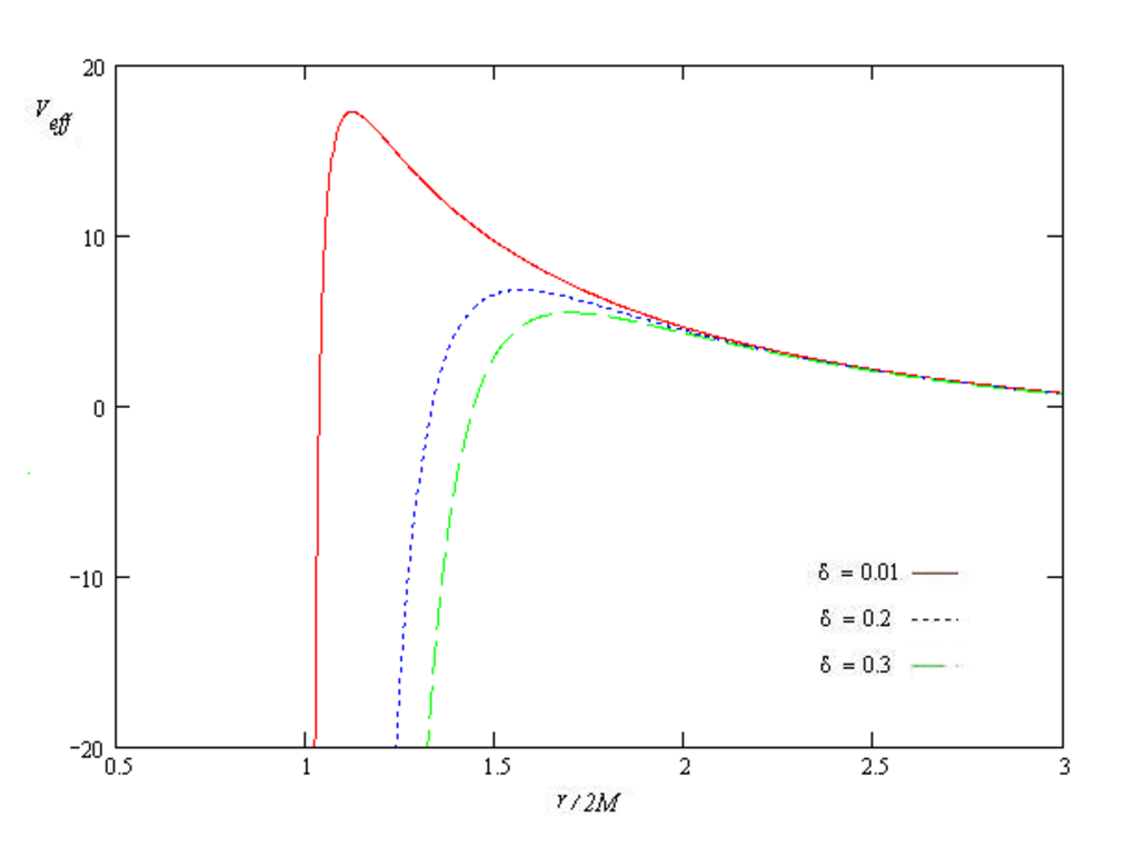
b) 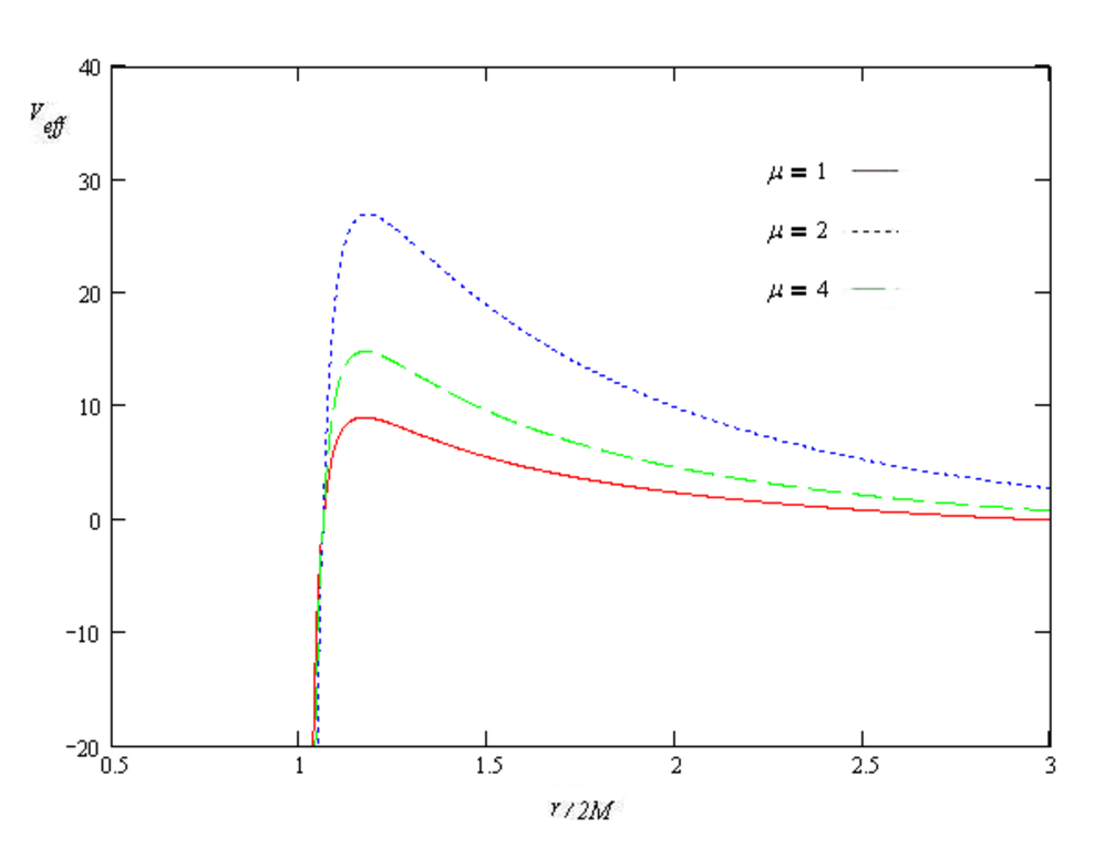
From the equation (29) one can easily get equations describing the motion of the test particle what is done below.
Trajectory of the charged particle around slowly rotating magnetized WH can be drawn from the following equation:
It is almost impossible to integrate equation (III) in general form. However one can get shape of the trajectory of the test particle by using basic assumptions and numerical integration. Figure 2 illustrates the shape of the trajectory of charged particles starting from sufficiently far distances towards the slowly rotating central object for different values of small parameter and zero momenta of the particle in infinity. From the presented figure 2 one can see that increase of the parameter makes gravitational field of the central object more stronger which forces test particle approach closer to the central object.

Radial motion of the charged particles near the slowly rotating magnetized WH can be described using the following equation derived from (29):
In paper [24] it was shown from the solution of equation of radial motion of particle in spherical symmetric spacetime of nonmagnetized WH that particles can make radial harmonic oscillations. We obtain here from equation (III) in the case of magnetized slowly rotating WH, that charged particles make radial anharmonic oscillations. The periods of that oscillations are presented in the Table 1. for the different values of the magnetic parameter and the parameter .
| 0.001 | 0.01 | 0.02 | 0.05 | 0.1 | |
|---|---|---|---|---|---|
| 4.02782 | 4.07698 | 4.11094 | 4.21451 | 4.39281 | |
| 4.41272 | 4.46564 | 4.52357 | 4.69716 | 4.9919 | |
| 4.93646 | 4.99437 | 5.05869 | 5.25325 | 5.58609 | |
| 5.22254 | 5.28301 | 5.35083 | 5.55727 | 5.91227 |
Finally we study periods of the circulating charged particle around slowly rotating magnetized WH (stability of the circular orbits will be discussed later in the next subsections) by using the following equation derived from (29):
Figure 3 shows the dependence of the period of the circulating particle from the magnetic dipole momenta of the WH for different values of the small parameter . The graphs justify that increase of the parameter cause particles to approach closer to the central object.

III.1 Stable Circular Orbits for Charged Particles
Special interest for the accretion theory of test particles around a slowly rotating wormhole with a dipolar electromagnetic field is related to the study of circular orbits which are possible in the equatorial plane when is zero. Consequently the right hand side of equation (30) vanishes:
| (35) |
along with its first derivative with respect to r
| (36) |
The radius of marginal stability, the associated energy and angular momentum of the circular orbits may be derived from the simultaneous solution of the condition:
| (37) |
From equations (35) and (36), one may find expression for energy
| (38) |
and expression for momentum
| (39) |
of charged test particles. Here we have used the following notations:
and
Now, inserting (38) and (39) into equation (37), one may obtain the basic equation
| (40) |
In this, we have used following additional notations:
The numerical solutions of the equation (40) will determine the radii of marginally stable circular orbits for slowly rotating wormholes with magnetic dipole momenta as functions of the parameter , the angular velocity , as well as of the magnetic dipole of the source. In the Table 2, we numerical solutions for the radii of the stable circular orbits of charged test particles for different values of the parameter and magnetic dipole moment of the wormhole. With the increase of the , radii of stable circular orbits shift to observer at the infinity, while existence of magnetic dipole moment and a possible increase in it displace the orbits to the gravitational source.
| 0.01 | 0.02 | 0.03 | 0.04 | 0.05 | |
|---|---|---|---|---|---|
| 7.81538 | 9.31114 | 10.3082 | 11.0739 | 11.7021 | |
| 6.31054 | 7.52564 | 8.34287 | 8.97572 | 9.49905 | |
| 4.86001 | 5.79180 | 6.41939 | 6.90621 | 7.30947 | |
| 3.90299 | 4.64910 | 5.15093 | 5.53995 | 5.86208 | |
| 3.18162 | 3.79127 | 4.19940 | 4.51495 | 4.77577 | |
| 2.93889 | 3.50249 | 3.87818 | 4.16793 | 4.40702 |
IV Astrophysical Applications and Conclusions
In this paper we consider electromagnetic field of slowly rotating WH i.e. neglecting quadratic and higher order terms of angular velocity we first find exact vacuum solutions of Maxwell equations in spacetime of slowly rotating magnetized WH. In the paper [14] it has been justified that electric charge could exist in WH and did not change the structure of the space-time around WH seriously, which gives us the right to consider the existence of magnetic dipole momenta of the WH due to possible motion of the electric charge.
Astrophysical processes and effects around black hole and WH different models are distinguishable such as absence of event horizon on WH, passage of the radiation and particles through WH, appearance of blueshift effect in addition to the gravitational redshift effect near WH etc (see for the details [11, 27]). In Ref. [12] circular orbits of test particles around a WH and their periods were studied. Here we extended these results to motion of charged particles and have shown the strong dependence of particle motion from WH shape parameter and magnetic field strength.
Here we address two basic question: are there any differences between astrophysical processes around WH and standard models for compact object? If there are so, how can we distinguish WH from other compact objects using observational data? To answer these questions we consider magnetic dipole momentum of the WH and develop the existing WH model constructed by [12]. For such models we perform a charged particle motion analysis around magnetized WH. Finally we can conclude that from astrophysical point of view the following differences between WH and standard compact objects can be detected observationally:
1. Oscillations of bodies in the vicinity of a WH throat (radial orbits) could give rise to a peculiar observational phenomenon. Signals from such sources detected by an external observer will display a characteristic periodicity in their spectra. All objects (stars, BHs) other than WHs absorb bodies falling onto them irrecoverably. Periodic radial oscillations are a characteristic feature of magnetized WHs as it was first shown by [11] for other WH models.
2. As it was shown by [11] the difference of the circular motion of particles around ReisnerNordström black hole and around the charged WH model described by [12] is negligible at (or more). Thus all conclusions about circular orbit around a WH are the same as in the limiting ReisnerNordström geometry at the corresponding distances. However, on the contrary for our WH model which has a magnetic dipole momentum one can easily obtain the difference on circular motion of charged particle around WH and compact object as stars, BH etc. As we have shown in subsection III.1 with the increase of the , radii of stable circular orbits shift from central object (WH) to observer at the infinity. From the numerical results given in Table 2. one can easily see that the influence of parameter on particle motion depends on the strength of magnetic field of WH: radii of the stable circular orbits differ almost 2 times bigger when , while this increasing almost disappears when magnetic field of WH is margin.
Acknowledgments
AAA and BJA thank the IUCAA for warm hospitality during their stay in Pune and AS-ICTP for the travel support through BIPTUN (NET-53) program. Authors also thank Dr. Anisul Usmani for useful comments and correcting the text of paper. This research is supported in part by the UzFFR (projects 5-08 and 29-08) and projects FA-F2-F079, FA-F2-F061 of the UzAS and by the ICTP through the OEA-PRJ-29 project and the Regular Associateship grant.
References
- [1] Bergliaffa, P. & Hibberd, K. E.2000, gr-qc/0006041
- [2] Beskin, V.S. 1990, Soviet Astron. Lett., 16, 286
- [3] Böhmer, C. G., Harko, T., & Lobo, F.S.N. 2008, Class. Quant. Grav, 25, 075016
- [4] Cabibbo, N. & Ferrari, E. 1962, Nuovo Cim., 23, 1147
- [5] Dadhich, N., Kar, S., Mukherjee, S., & Visser, M. 2002, Phys. Rev. D, 65, 064004
- [6] Dadhich, N. & Turakulov, Z.Ya. 2002, Class. Quantum Grav., 19, 2765
- [7] Deutsch, A.J. 1955, Ann. Astrophys., 1, 1
- [8] Dey, T. K. & Sen, S. 2008, Mod. Phys. Lett. A, 23(13), 953
- [9] Harko, T., Kovács, & Z., Lobo F.S.N. 2008, Phys. Rev. D, 78, 084005
- [10] Jamil, M. & Rashid M. 2008, astro-ph/08050966v2
- [11] Kardashev, N. S., Novikov I.D., & Shatskii A.A. 2007, Int. J. Mod. Phys. D, 16, 909
- [12] Kardashev, N.S., Novikov, I.D., & Shatskii, A.A. 2006, Astronomy Reports, 50, 601
- [13] Kashargin, P. E. & Sushkov, S. V. 2008, Phys. Rev. D, 78, 064071
- [14] Kim, S.-W. 2005, Nuovo Cimento B, 120, 1235
- [15] Kim, S.-W. & Lee, H. 2001, Phys. Rev. D, 63, 064014
- [16] Konno, K. & Kojima, Y. 2000, Prog. Theor. Phys., 104, 1117
- [17] Kuhfittig, P. K. F. 2008, gr-qc/08061194v1
- [18] Lobo, F. S. N. 2005a, Phys. Rev. D, 71, 084011
- [19] Lobo, F. S. N. 2005b, Phys. Rev. D, 71, 124022
- [20] Morris,M. S., Thorne, K. S., & Yurtsever, U. 1988 Phys. Rev. Lett., 61, 1446
- [21] Morris, M. S. & Thorne, K. S. 1988, Am. J. Phys., 56, 395
- [22] Muslimov, A.G. & Tsygan A.T. 1992, Mon. Not. R. Astron. Soc., 255, 61
- [23] Muslimov, A.G. & Tsygan A.T. 1990, Soviet Astr., 34, 133
- [24] Novikov, I.D., Kardashev, N.S., & Shatskii A.A. 2007, Physics Uspekhi, 50, 965
- [25] Rezzolla, L., Ahmedov, B.J., & Miller, J.C. 2001a, Mon. Not. R. Astron. Soc., 322, 723; Erratum 2003, 338, 816
- [26] Rezzolla, L., Ahmedov, B.J., & Miller J.C. 2001b, Found. of Phys., 31, 1051
- [27] Shatskii, A.A. 2007, Astronomy Reports, 51, 81
- [28] Sushkov, S. 2005, Phys. Rev. D, 71, 043520
- [29] Teo, E. 1998, Phys. Rev. D, 58, 024014
- [30] Visser, M. 1995: Lorentzian Wormholes: from Einstein to Hawking (American Institute of Physics, Woodbury)
- [31] Visser, M., Kar, S., & Dadhich, N. 2003, Phys. Rev. Lett., 90, 201102