Freedom and Constraints in the K3 Landscape
Abstract
We consider “magnetized brane” compactifications of the type I/heterotic string on K3 with background fluxes. The nonabelian gauge group and matter content of the resulting six-dimensional vacua are parameterized by a matrix encoding a lattice contained within the even, self-dual lattice . Mathematical results of Nikulin on lattice embeddings make possible a simple classification of such solutions. This approach makes it possible to explicitly and efficiently construct models in this class with a particular allowed gauge group and matter content, so that one can immediately “dial-a-model” with desired properties.
1 Introduction
In this paper we consider a very simple class of string vacuum solutions associated with supersymmetric 6-dimensional low-energy physics. Models of the type we consider here are characterized by an intersection matrix associated with an even, self-dual lattice. We use theorems on lattice embeddings to give a characterization of the space of allowed models. This gives a concrete realization of a piece of the landscape in which models can be conveniently characterized and identified based on simple features of their low-energy physics. A brief summary and introduction to the main technical results of the paper is given in Section 1.1.
While quite far from the physically observed world in which supersymmetry is broken and space-time is 4-dimensional, the simple mathematical structure described here may help provide insight into some aspects of the larger space of string vacuum solutions, and in particular into the question of whether low-energy physics is constrained by string theory. To put this work in context, a brief discussion of the string vacuum problem and some of the motivation for this work is given in Section 1.2. Those uninterested in landscape philosophy may skip Section 1.2.
1.1 Introduction and outline of results
The models we consider in this paper are type I/heterotic string theory compactifications on a K3 surface. Such compactifications are characterized by an bundle33 3 The case of the heterotic string can be treated in a completely analogous manner. The general story remains unchanged, but the specific low-energy theories obtained are different. over K3. In type I language, the background contains an orientifold 9-plane and 16 D9-branes whose charges combine to cancel the ten-form RR tadpole. In a curved background, such as a K3 surface, there is also a six-form tadpole (D5-brane charge) [1] that can be cancelled by introducing world-volume fluxes for the gauge fields on the D9-branes. These fluxes on the D9-branes thread 2-cycles in the K3 surface and produce D5-brane charge equal to the instanton number of the flux configuration [2, 3].
Models of the type considered here, with fluxes on D9-branes in type I string theory encoding lower-dimensional D-branes wrapped on various cycles, are known as “magnetized brane models”. Choosing different fluxes on different D9-branes in these models leads to chiral fermions in the dimensionally reduced theory [4, 5]. These models were developed in the type I context in [6] and have been widely studied in the literature. Reviews of this work and further references appear in [7].
In general, the flux in the gauge fields on the D9-branes can be nonabelian, but we restrict attention here to the simplified class of configurations where only fluxes, corresponding to fluxes on individual D9-branes, are turned on. Mathematically, this means that the gauge bundle has a curvature that can be described in terms of a direct sum of abelian connections on the individual D9-branes. In the more general case of nonabelian vector bundles a similar story holds, but the technical details are more complicated. Recent related work on heterotic line bundle models appears in [8, 9, 10].
On a torus, magnetized brane models are T-dual to intersecting brane models [11]; the D9-brane world-volume fluxes are T-dual to the tilts of the diagonal intersecting branes on the dual torus. (Intersecting brane models are also reviewed in [7].) This duality with intersecting brane models provides useful intuition for the physics of magnetized brane models, although on a smooth K3, T-duality is replaced with mirror symmetry, which is harder to describe explicitly. Part of the motivation for this work was to extend the systematic analysis of intersecting brane model solutions on toroidal orbifolds to more general smooth Calabi-Yau spaces where intersecting brane models are not particularly well defined, as discussed in Section 5 of [12].
For the magnetized brane models we consider here, each D9-brane carries a separate gauge field strength . This field strength takes quantized values when integrated over any 2-cycle of K3 and thus, when suitably normalized by the unit of charge , lives in the integral 2-cohomology of the K3 surface, i.e., . The cohomology group has the structure of a lattice, with a natural inner product given by the wedge product in cohomology, which is Poincaré dual to the intersection number of 2-cycles in homology. By a lattice in this paper we will always refer to a vector space over carrying an integral, symmetric inner product. For a K3 surface, the lattice defined by the cohomology group is the unique even, self-dual unimodular lattice of signature (3,19), denoted . A review of the structure of this lattice and some basic definitions relevant for lattices are given in A.
Any vacuum solution of this type is therefore associated with a set of vectors (not necessarily distinct) in the lattice . Since we have turned on fluxes, the gauge group in the 6D theory is broken from to the commutant of the fluxes. If we were to turn on 16 distinct ’s the gauge group would be broken to . The tadpole constraint in fact restricts the number of nonzero ’s to be at most 12 for smooth K3 geometries. Note that the vectors need not be distinct, and some of them could be equal. When some of the are equal, the gauge group on the branes is expanded to a nonabelian group. Let denote the distinct, non-zero vectors among the set . We use the (with hats) to denote the fluxes on each D9 brane, where the index runs over individual branes, and the notation (no hats) to denote the distinct fluxes among these. In the most general situation, we have magnetized stacks of equal fluxes where and all the are distinct. By a magnetized stack we mean a set of D9-branes each with the same value of (non-zero) flux turned on. The stack of branes with will be called the unmagnetized stack.
The gauge group and matter content of the dimensionally reduced 6D theory is completely determined by the sizes of the flux stacks and the topological invariants of the fluxes, where denotes the inner product on the lattice. The gauge group and matter content can be enhanced when the K3 surface becomes singular. We focus in this paper on smooth K3 compactifications, where the gauge group is given by a product of unitary groups ; the unitary groups arise from the magnetized stacks and the orthogonal group arises from the unmagnetized stack. (Note that generally the factors in are anomalous and get masses through the Green-Schwarz/Stueckelberg mechanism). The number of matter fields in the various allowed representations of the gauge group can be written in terms of the intersection matrix and the stack sizes . Thus, the stack sizes and intersection matrix parameterize the possible low-energy theories realizable in this construction.
To understand the range of models possible, we therefore need to know what intersection matrices and multiplicities can be realized in string theory. This question can be conveniently reformulated in the language of lattice embeddings. We can think of the vectors as generating a lattice of rank with inner product determined by the matrix .44 4 The lattice is required to contain the integral vector to avoid global anomalies. For a smooth K3 compactification, we also require to not have any vectors with norm-squared . The main result of this paper is the conclusion that existing theorems on lattice embeddings, due to Nikulin and earlier authors, provide a fairly complete characterization of the space of abelian magnetized brane models on K3 through the classification of allowed intersection matrices . The vanishing of the six-form R-R tadpole gives a constraint on the trace of the full intersection matrix . This becomes when we rewrite the sum over branes into one over stacks. Low-energy supersymmetry further requires the lattice to be negative-definite. Up to these constraints, Nikulin’s results on lattice embeddings essentially state that any desired intersection matrix can be realized in a K3 compactification, except possibly in cases where the rank of the matrix is 11 or 12. Furthermore, the realization of a specific intersection matrix is almost unique up to automorphism (relabeling) of the K3 cohomology lattice, with the ‘‘almost’’ caveat arising from some discrete redundancies55 5 Equivalent discrete redundancies were recently encountered in analysis of dyon models [13]. associated with a finite number of possible refinements (overlattices) of the lattice .
The upshot of this analysis is that for this family of models the intersection matrix provides a complete means of classifying the range of possible models according to simple features of their low-energy physics. The methods described here can be used to enumerate the models in the class in a straightforward way, either to search for models with specific features or to perform a statistical analysis on the class of models. Furthermore, the intersection matrix provides a straightforward way to directly construct all models with a particular desired feature. For example, one might wish to construct all models with a particular group, like as a subgroup of the full group and at least 3 chiral fermions in the bifundamental . This can be formulated as a constraint on the intersection matrix , so that all models with the desired feature can immediately be constructed or enumerated. Again, this could be useful either for model-building purposes or for statistical analysis of the space of models.
The analysis of this paper thus gives a particularly simple example of a region of the landscape where models can be easily classified and explicitly constructed. It is interesting to contrast this with other types of models where classifying all allowed vacuum solutions is difficult or impossible with current methods. In some cases, identifying the complete set of models with a particular set of physical features may be computationally difficult or intractable. For example, consider the closely related family of intersecting brane models on a toroidal orientifold. The simple and popular toroidal model [14] has been studied in many papers over the last decade and gives rise to semi-realistic 4D theories with a gauge group containing the standard model gauge group and 3 generations of chiral matter fields [15, 16, 17, 18, 19, 7]. Due, however, to the presence of supersymmetric branes with tadpole contributions of mixed signs in this class of models, a complete understanding of the space of allowed models poses a significant challenge. In [20], a systematic search using a year of computer time sampled a large number of vacua in this class. In [12], it was proven that the set of inequivalent models in this class is finite. The classification of these models has now been completed and will appear in [21]. In this toroidal orbifold construction, finding the set of models with a particular physical feature can be quite a nontrivial problem. (For example, finding all models with gauge group containing the subgroup poses a significant computational challenge, whose solution appears in [21]). In the class of K3 models considered in the present paper, on the other hand, such a construction is relatively straightforward. The constraint on the gauge group can be imposed on the stack sizes and intersection matrix , and all satisfying this constraint can immediately be constructed and tabulated (as discussed in Section 7).
In the following subsection we summarize some outstanding issues related to the large landscape of string vacua and the problem of predictability in this context. In brief, the message of this paper is that in this special corner of the string landscape the space of string theory compactifications has a very simple organizing principle. Given the parameterization of the allowed space of models in terms of the intersection matrix , in this region of the landscape there is both freedom and constraint, in that any negative-semidefinite matrix that determines an even lattice of rank can be realized in string theory, provided that has no vectors and satisfies the linear tadpole constraint. Furthermore, up to some limited discrete redundancy, any allowed low-energy physics structure is realized in a unique way up to dualities. While such a simple framework is unlikely to extend to the whole string landscape in any foreseeable fashion, this gives an example of a part of the landscape where underlying mathematical structure gives great simplicity to the discrete variety of allowed string theory solutions.
The structure of the rest of this paper is as follows: In Section 2 we review the basic geometry of K3. In Section 3 we describe the class of type I magnetized brane models of interest. The 6D dimensionally reduced physics of these models is described in Section 4. The existence of models for any negative-semidefinite even matrix of rank that satisfies the tadpole constraint is demonstrated using Nikulin’s theorems in Section 5. A systematic approach to enumeration of models including the determination of discrete redundancies is presented in Section 6, along with some explicit examples. In Section 7 we show how all models with particular desirable features such as a specific low-energy gauge group or matter content can be efficiently enumerated. Concluding remarks appear in Section 8. Appendices contain additional technical material on the structure of the lattice and Nikulin’s lattice embedding theorems.
Note for version v4: We have made the following significant changes to this version: a factor of two error in the tadpole condition has been corrected, we have restricted ourselves to smooth K3 compactifications by eliminating vacua that involve vectors in the Picard lattice of the K3 surface, and the mod 2 constraint from the Freed-Witten global anomaly has been included. These modifications do not affect the central conclusion of this paper that string vacua in this part of the landscape can be characterized through the existence of lattice embeddings. However, some specific quantitative statements regarding enumeration of models have been revised. We are grateful to Edward Witten, Ilarion Melnikov and the authors of [22] for helpful communications regarding these issues.
1.2 Predictions and the vacuum problem
It has been known since the early days of string theory that the space of supersymmetric string vacua is vast. For example, for any Calabi-Yau complex 3-manifold there is a continuous moduli space of supersymmetric string vacuum solutions. More recently, the experimental observation of a positive nonzero cosmological constant has led to a new effort to understand the “landscape” of metastable string vacua with positive cosmological constant. Incorporation of fluxes and other mechanisms can stabilize the continuous moduli of a space of vacuum solutions, and in principle with the breaking of supersymmetry the cosmological constant can be lifted to a positive value. The exponentially large number of ways in which fluxes can be introduced gives an exponentially large number of candidate string vacua, whose enormous multiplicity has been invoked as an explanation for the existence of solutions having a positive cosmological constant with the observed small value. Reviews of developments on the landscape of flux compactifications appear in [23].
In considering the apparent enormous multiplicity of stable and metastable string theory vacuum solutions, the problem of extracting predictions for the low-energy theory becomes increasingly acute. It has been suggested that statistical analysis of the space of allowed models may provide fruitful insights [24]. In the absence of a true understanding of background-independent dynamics of string theory, however, it is as yet very difficult to extract physically meaningful predictions from the statistics of vacua or to make progress on other proposed vacuum selection mechanisms.
Thus, without some dramatic new insight into the global and temporal dynamics of string theory, at the present the clearest course of action is to consider the full space of possible string solutions. It is possible that string theory imposes absolute constraints on low-energy physics. If present, such constraints should be observed in any sufficiently broad family of string vacua. Here we use a very simple framework to illustrate the question (more statistical approaches to this kind of question have recently been taken in [25, 26]; for a more bottom-up perspective see [27]). Given some set of string vacua (for example, intersecting brane models on a particular toroidal orbifold), and a set of low-energy observables (for example, the gauge group, matter content, Yukawa couplings etc.), there are roughly two extremes according to which the observables can be distributed in the set of vacua.
A) “Anything goes”. In this extreme, essentially all possible values of the observables in question can be realized within the set of vacua . For continuous observables like masses and couplings, this might mean that any possible combination of masses and couplings could be realized to a particular level of precision dependent on the number of vacua in the set . (In some cases there may be a fixed range within which this freedom is realized, so that distributions of type A may really be best described as B “bounded”)
C) “Constraints”. In this extreme, there are absolute constraints on the set of observables. For example, one could imagine that for a given set of vacua, any model that contains has precisely 3 generations of bifundamental “quark-like” matter fields. Or one might find that a constraint on a combination of several masses and couplings gives one of these parameters as a function of the others.
To make a specific quantitative prediction from string theory one would need to show that for all possible sets of vacua, a common constraint of type C arises in the low-energy theory. Of course, the set of vacua within our current range of understanding is probably only a tiny fraction of the full range of string solutions, so we cannot reasonably show this for all sets of vacua. If, however, we can demonstrate that in a number of ostensibly unrelated corners of the landscape there are common constraints on the low-energy physics, this would represent a hypothetical universal constraint, which could be tested by examining other classes of string solutions.
On the other hand, to show that a given set of observables, taken in isolation, is not constrained by string theory, it suffices to find a single class of string models in which situation A holds. For example, in [20, 12, 21] the space of supersymmetric intersecting brane models on the toroidal orientifold was studied systematically. Considering only the low-energy gauge group and numbers of matter fields in different representations, this class of models seems to give a distribution best described by A), “anything goes”. Although there is a maximum to the size of the gauge group and number of matter fields that bounds the range of the distribution and produces a sparse “tail”, small groups like , can all be realized in many ways as part of the full gauge group in this construction with arbitrary (but not too large) numbers of chiral matter fields in the representation. This confirms, as has long been known, that string theory cannot uniquely determine the gauge group and number of generations of matter without additional constraints (like perhaps SUSY breaking). Of course, for this particular orientifold construction, the total number of possible models is somewhat limited. As shown in [21], the number of distinct ways the gauge group can be realized as a subgroup of the gauge group with 3 generations of “quarks” in this class of models is limited to several thousand. Thus, the “anything goes” nature of the general distribution is limited by the finite sample size. Indeed, while a number of semi-realistic models have been found in this framework [15, 16, 17, 18, 19], these generally have extra massless chiral exotic fields, and differ from the standard model in observable ways. A larger sample is needed to reproduce more detailed features of the standard model, even in the absence of definitive stringy constraints. Such larger samples can be found, for example, by generalizing to arbitrary Calabi-Yau geometries or Gepner model constructions [28].
To date there are no conclusively demonstrated broad constraints on the space of low-energy theories that can be realized in string models (though some interesting suggestions leading towards such constraints have been made in [29]). Thus, in order to see whether string theory produces constraints on low-energy theory anywhere in the landscape it may be fruitful to begin with the simplest classes of string compactifications. The string vacuum solutions we consider here, associated with type I magnetized branes on K3, live in such a simple, and hopefully easier to analyze, corner of theory space. The resulting vacua, which are 6-dimensional and supersymmetric, are far from the physically observed world. These models obey some specific constraints, but can vary freely subject to these constraints Specifically, we find that the gauge group and matter content of the low-energy theory have a particular dependence on the stack sizes and intersection matrix parameters . Any intersection matrix subject to the constraint that the lattice it determines is even, negative-definite, has no norm-squared vectors, and satisfies a simple tadpole constraint, can be realized in an almost unique way as a string compactification, at least in cases when rank .
The simple mathematical structure found for this class of models, and its consequences for the part of the landscape where this analysis is relevant, suggests that a search for a similar decomposition of the landscape distribution into constraints and freedom may be helpful in a broader class of string vacua. Such analysis might help to address the question of whether, even in a simple supersymmetric and higher-dimensional context, string theory has the potential to constrain any part of the low-energy field theory arising from compactification.
2 Some basic facts about K3 surfaces
In this section we review the basic properties of K3 surfaces that are relevant to our discussion. A more detailed exposition complete with references can be found in Aspinwall’s lectures on K3 surfaces [30]. A K3 surface can be defined as a compact, two complex dimensional, simply-connected Calabi-Yau manifold. In other words, is a compact, simply-connected complex surface with trivial canonical bundle. Like all Calabi-Yau manifolds, any K3 surface admits a Ricci-flat Kähler metric. The reason Calabi-Yau manifolds are of interest is that they are an exact solution of the superstring equations of motion and they preserve some of the supersymmetry of the ten-dimensional theory. There are many thousands of topologically distinct Calabi-Yau three-folds known [31] and it is not yet clear whether the total number of such manifolds is finite or infinite. Two-dimensional compact Calabi-Yau manifolds are severely constrained in this regard and in fact there is only one simply-connected Calabi-Yau surface (the K3 surface) up to diffeomorphism. Thus, all K3 surfaces have the same topology which can be determined by studying any specific one. In particular, the Betti numbers are completely determined and they are . For a K3 surface is torsion-free and therefore has the structure of a lattice, by which we mean a free -module, i.e (as a free abelian group).
The lattice has a natural integral, symmetric, bilinear form defined as the intersection number of the two 2-cycles . The intersection number is a well-defined quantity on homology classes [32] and satisfies (integral), (symmetric) and (bilinear) for all and . A lattice with an integral, symmetric, bilinear form is said to be even if for all , is an even integer. is self-dual if . Given a basis for the lattice , the bilinear form defines a matrix . The signature of is defined as , where and are the number of positive and negative eigenvalues of respectively.
It can be shown that the lattice (with the bilinear form ) associated with any K3 surface is an even, self-dual lattice of signature [30]. In fact, there is precisely one such lattice with these properties up to isometry33 3 Two lattices and are isomorphic if there exists a bijective map . If preserves the bilinear form then is said to be an isometry.; this lattice is denoted by (See Appendix A). Poincaré duality implies that the lattices and are isometric55 5 The Poincaré dual of a 2-cycle is a closed two-form such that for every 2-cycle C, . Poincaré duality maps the intersection product in homology to the wedge product of forms in cohomology [32]. Given closed 2-cycles and their Poincaré duals , we have . and that . For the rest of the paper, we will use the notation to denote the bilinear form on a lattice, which in this case would be the intersection number in homology, or the wedge product of forms in cohomology.
Given a complex structure on , there exists a globally defined, nowhere vanishing, holomorphic two form . A complex structure defines a Hodge decomposition of the lattice as . and is defined only up to scaling by a non-zero complex number. The Hodge decomposition determined by uniquely specifies the complex structure. We can write , where . The elements and are constrained because satisfies
| (1) |
Therefore, and satisfy and . These conditions imply that the real plane spanned by and in is positive definite. Thus, the complex structure on is determined by a positive-definite two-plane in the space . The Kähler form is a real, closed form and satisfies
| (2) |
The above equations imply that the holomorphic two-form and the Kähler form determine a positive-definite three-plane in .
3 Type I/Heterotic on K3
We wish to construct vacua with chiral supersymmetry (8 real supercharges) starting with the type I or heterotic string theory on a K3 surface . The type I and heterotic string33 3 The gauge group is really Spin(32)/ and not for both the type I and the heterotic string. See [33, 34] for further discussions of this point. theories are equivalent under a strong-weak duality [35]. The low-energy effective action of both string theories is type I supergravity. Since our analysis is carried out using the effective action alone, it applies to both the type I and the heterotic string. Some calculations are more transparent in the heterotic string, while the type I string gives an intuitive picture of the gauge group in terms of D9-branes. In this section we discuss the constraints imposed by tadpole cancellation and low-energy supersymmetry. Readers familiar with these constraints can skip to the summary at the end of this section.
3.1 Tadpole cancellation
In the context of the heterotic string, the tadpole constraint arises from integrating the Bianchi identity for the NS-NS field over the K3 surface. In the type I theory the same constraint arises from the equation of motion for the six-form RR potential, including the Wess-Zumino couplings of the O9-plane and the D9-brane in the presence of world-volume fluxes. Since these are dual descriptions of the same system, both approaches must yield the same answer. We summarize the calculation of the constraint here in heterotic language, which is perhaps more transparent, following [36]. We then summarize the physical content of this constraint as interpreted in the type I theory.
The Bianchi identity in the heterotic string is [38]
| (3) |
where and denote the curvatures of the tangent bundle and gauge bundle respectively, and the trace is to be taken in the vector representation. Integrating this equation over we obtain
| (4) |
This is an equality of the Pontyagin classes of the gauge bundle and tangent bundle integrated over . For a K3 surface the right hand side evaluates to -48 [37], and this leaves us with the tadpole constraint
| (5) |
In the type I language, the orientifold action fixing all space-time points gives an O9-plane with ten-form R-R charge . The gauge group lives on the 16 D9-branes which, along with their orientifold images, must be added to cancel the R-R charge from the O9-plane. Due to the non-zero Riemann curvature of S, the gravitational couplings of the D9-branes and O9-plane [1, 39] induce a net nonvanishing six-form R-R tadpole. We cancel the tadpole by turning on background world-volume fluxes with the appropriate instanton number on the D9-branes. These world-volume fluxes on the D9-branes thread 2-cycles in S and have D5-brane charge equal to the instanton number of the flux configuration [2, 3].
3.2 bundles and Dirac quantization
We restrict our attention to gauge bundles that are sums of bundles for the sake of simplicity. is a rank 16 group and has sixteen factors. Let denote the sixteen anti-Hermitian Cartan generators in normalized so that . The curvature form can be expanded in this basis as where are closed 2-forms, some of which could be zero. We know that fluxes threading compact 2-cycles inside are subject to Dirac quantization. With our normalization conventions this implies the integrality of the class
| (6) |
In terms of the , the tadpole condition (5) reads
| (7) |
Here the denotes the intersection product on the lattice as explained in Section 2.
It is useful to keep in mind the interpretation in terms of the type I theory. A single D9-brane with a world-volume flux has an orientifold image with flux . The brane and its image together form a single, dynamical type I D9-brane with Chan-Paton indices. The type I theory contains sixteen D9-branes with Chan Paton indices and we therefore can turn on a maximum of sixteen independent fluxes .
3.3 Supersymmetry constraint
Since we demand that the six-dimensional vacua have supersymmetry, the gauge bundle is constrained. It is well known [38, 42] that to preserve supersymmetry the curvature form must satisy . Here and are holomorphic coordinates on and is the Kähler metric. In terms of the fluxes, this implies for each . The first two conditions are equivalent to the global conditions
| (9) |
This is because on a K3 surface, any (2,0) form is proportional to up to a complex constant; the integral conditions (9) imply that this constant of proportionality is zero, and therefore that the local conditions are satisfied. This implies that is a -form, and therefore that the corresponding bundle is holomorphic. Given a holomorphic bundle with curvature form , the third (local) condition is satisfied iff the global constraint is true [43]. Thus, supersymmetry places three (global) conditions on the curvature two-form
| (10) |
We now ask the question — “Given a set of line bundles on K3 specified by the lattice vectors in , does there exist a choice of and so that supersymmetry is preserved?”. We know from our discussion in Section 2 that and span a positive-definite three-plane in the space . Since the lattice has signature (3,19), if we restrict the to a negative-definite plane (dimension ), there always exists a real, positive definite, 3-plane orthogonal to it. We can always choose and to lie in the positive definite 3-plane. Therefore, the only constraint from supersymmetry is that the lattice vectors generate a negative-definite sublattice in . This implies in particular that . Since the lattice is even, we have . When the Poincaré dual homology class , or its negative , contain an irreducible rational curve [30]. The supersymmetry conditions (10) require that this holomorphic curve have zero volume, thereby rendering the K3 surface singular. In order that be smooth we must require that the lattice , known as the Picard lattice, not contain any norm-squared vectors. This can be ensured by demanding that the real vector space spanned by the (a sub-space of ) not contain any integral vectors with norm-squared . In particular, this implies that . Note that the vectors need not be linearly independent, or even distinct, and so are not necessarily a basis of minimal dimension for the lattice they generate. The tadpole constraint (7), , can only be satisfied if at least four ’s are zero. Therefore, even though the gauge group has sixteen factors, at most twelve of them can be turned on.
3.4 Summary of constraints
The tadpole condition (5) can be satisfied by turning on background world-volume fluxes threading various 2-cycles in the K3. We focus on world-volume fluxes for simplicity. Dirac quantization implies that the fluxes, appropriately normalized, are vectors in the integral cohomology lattice . For each factor, we have a lattice vector ; in terms of these vectors , the tadpole condition is simply . Supersymmetry requires that the non-zero vectors (not required to be linearly independent, or distinct) generate a negative-definite sublattice of . The K3 surface is smooth only if the lattice contains no norm-squared vectors, which implies that . This in turn implies that we can have at most twelve non-zero . Let denote the lattice generated (over ) by the vectors and . Then,
| (11) | ||||
When these constraints are satisfied, we have a consistent string compactification on a smooth K3 surface that satisfies the equations of motion in the supergravity approximation. That is, for any set of fluxes satisfying (11), there exist choices of complex structure and Kähler form on K3 satisfying (10). The moduli space of these solutions is restricted by the choice of fluxes, since the complex structure and Kähler form of the K3 surface are constrained to be orthogonal to the lattice generated by the fluxes . While we have restricted our attention to smooth K3 compactifications, it is possible that some of the singular compactifications are consistent; we comment on this in the following section.
4 Six-Dimensional Physics
In this section we describe how the parameters of the compactification discussed in the previous section affect the low-energy physics. These six-dimensional, supersymmetric compactifications of the string on K3 have been studied earlier in [4, 9, 10]. In six-dimensional theories with supersymmetry, there are four kinds of massless multiplets (see Appendix B of [44]), listed in Table 1.
| Multiplet | Matter Content |
|---|---|
| SUGRA | |
| Tensor | |
| Vector | |
| Hyper |
The SUGRA and the tensor multiplets are uncharged under the gauge group, and the vector multiplet transforms in the adjoint. In six dimensions, the CPT conjugate spinor has the same chirality as the spinor. This implies that chiral fermions must always be charged under a real representation of the gauge group. The (chiral) hypermultiplet therefore transforms under a real representation.
4.1 Gauge group and matter content
Turning on fluxes breaks the down to the commutant of the for which . As discussed in Section 3.3, supersymmetry allows us to turn on at most twelve . Since at least four of the are zero, the gauge group always has an unbroken subgroup. If we choose twelve distinct nonzero ’s, the gauge group is broken to . When some of the ’s are equal to each other one obtains unitary groups. In the type I picture, this would mean that a stack of several D9-branes have the same background flux turned on. For example, with and , the commutant is . In general, the gauge group in these compactifications is with . This pattern of breaking is accomplished by having stacks, each with D9-branes where is an index for the stacks . The factors in the gauge group are generally anomalous due to the couplings with the two-form potential . However, in some cases, there are linear combinations of the factors that remain anomaly-free. In what follows we do not address the question of precisely which are lifted, and we simply retain the factors in the gauge group as it does not affect the classification and enumeration of vacuum solutions. We reserve the indices to denote individual D9-branes and the indices to denote stacks of branes.

We have restricted ourselves to smooth K3 surfaces since we are working in the supergravity limit. When the lattice spanned by the flux vectors contains the root lattice of an A-D-E gauge group, the K3 surface develops the corresponding A-D-E singularity [30]. The root lattice of an A-D-E group is generated by norm-squared vectors; as discussed earlier, the supersymmetry conditions (10) require the corresponding rational curves to zero volume, resulting in a singular K3 surface. When one of the flux vectors satisfies the zero-volume rational curve also supports instanton fluxes. In the absence of instanton flux, the classical A-D-E singularity is smoothed out by a strongly coupled worldsheet theory [45]. In the absence of a singularity, coincident small instantons enhance the gauge group by a factor , as shown in [2]. When small instantons coincide with an A-D-E singularity, it was shown in [47, 48, 49, 50, 46] that the coalescence of sufficiently many instantons can lead to a further enhancement of the gauge group, with additional hyper and tensor multiplets. In our case, small instantons with carry the same six-form charge as D5 branes, and therefore there may be a gauge enhancement of at least , with further enhancement possible from the A-D-E singularity. It is not clear whether these singular compactifications are consistent string vacua, and we leave the further study of these singular models to future work.
The matter content is easily visualized in the type I picture, as shown in Figure 1 where we have depicted a two-stack model. The gauge group is with and . We have two stacks containing and D9-branes, with distinct fluxes characterizing the two stacks. The remaining branes do not have any flux on their world-volume. We denote the stacks and their orientifold images as 1, 2, 1’, 2’ and 3,3’ respectively in Figure 1. The strings that stretch between and correspond to the vector multiplet and transform in the adjoint of and respectively. The strings (and their CPT conjugate strings) are charged in the representation of . There are also strings that stretch from a brane to the orientifold image of another brane. The strings transform in the bifundamental . The strings in the transform in the two-index antisymmetric representation of . The and strings transform in the and the representations respectively.
The massless matter content in these models can be computed using the Atiyah-Singer index theorem [4], [9], [10]. For example in the sector, the ends of the string carry charge under the bundle associated with the two branes to which the string is attached ( determines the normalization of the Lie algebra generators and is defined in section 3.2). The index theorem [37] gives the net number of normalizable, fermion zero modes in the presence of this background gauge field.
| (12) | |||||
| (13) |
Therefore, there are 6D hypermultiplets in the representation. This number is positive only when , which is consistent with the smoothness condition on , i.e. there are no integral norm-squared vectors. The number of massless multiplets in the other representations can be computed in an analogous manner. For a more general model, one can compute the above index for every pair of stacks ; the results of this computation are shown in Table 2. In addition, the closed string sector gives the six-dimensional SUGRA multiplet, 1 tensor multiplet and 20 neutral hypermultiplets [44]. The important thing to note is that all the massless matter content is determined by inner products of the lattice vectors . Defining the intersection matrix , the low-energy spectrum is thus completely determined by , with the gauge group determined by the stack sizes . It is interesting to note that requiring the number of multiplets as determined by the matrix to be non-negative imposes a weak form of the smoothness criterion on : the vectors , must have norm-squared .
| Representation | Number of hypermultiplets |
|---|---|
| Antisym. + c.c | |
| Neutral | 20 |
4.2 Anomaly cancellation
The anomalies in supersymmetric 6-dimensional theories can be cancelled by a generalization of the Green-Schwarz mechanism, as long as the and terms in the anomaly 8-form vanish. This computation was first carried out in [4], and more recently in [48, 9, 10]. The coefficient of the term, which corresponds to the purely gravitational anomaly** * In 6D theories, the CPT conjugate of a spinor has the same chirality as the spinor. As a result when a 6D field theory is coupled to gravity, in general there are purely gravitational anomalies [38]., is proportional to , where ,, are the number of hypermultiplets, vector multiplets and tensor multiplets respectively [44]. For the compactifications we consider, the closed string sector fixes and contributes 20 gauge-neutral hypermultiplets (from the K3 moduli). The gravitational anomalies vanish when , if we only count the multiplets from the field theory. It is easily checked that all our models satisfy this anomaly constraint.
Consider stacks, each of multiplicity and flux vectors satisfying the tadpole condition . The gauge group is with . The matter content is summarized in Table 2. The number of vector multiplets is for each factor and for the .
| (14) |
To obtain the number of hypermultiplets, we simply multiply the numbers in Table 2 with the dimension of the representation. This gives
Thus, all the models we construct satisfy the condition and are anomaly free.
5 Existence of solutions from lattice embeddings
We have now given a simple mathematical characterization of abelian magnetized brane models on K3. These models are specified by a set of lattice vectors , not necessarily linearly independent, which along with generate a negative-definite sublattice in . Each lattice vector is associated with identical abelian fluxes on a stack of D9-branes. These lattice vectors and multiplicities satisfy the tadpole condition
| (15) |
As shown in section 4.1, the gauge group and matter content of the resulting 6-dimensional supersymmetric theory depend only on the multiplicities and the intersection matrix .
We are now interested in finding a simple way of classifying all models of this type. In particular, in order to study the physics of this class of string compactification, we would like to know the answers to the following two questions:
(I) What combinations of multiplicities and intersection matrices can be realized in string theory?
(II) For those and which can be realized, in how many inequivalent ways can models with this data be constructed?
The equivalences referred to here are changes of basis of the lattice , which correspond to (large) diffeomorphisms of the K3 surface55 5 This is the Torelli Theorem for K3 surfaces [51]. There is a simple analogy with the case of the 2-torus. is a lattice with an anti-symmetric bilinear form . Automorphisms of this lattice form the group , which is the group of large diffeomorphisms of . See also related discussions in [30, 52].. The questions above essentially amount to whether the lattice defined by the intersection matrix 99 9 The vectors need not be linearly independent, therefore, the matrix does define a lattice, but is not the inner product matrix associated with the lattice . This turns out to be a minor subtlety and we address this issue in more detail in Section 6. can be embedded in the 2-cohomology lattice of K3, and whether such an embedding is unique. We begin with the simple case where there is only a single nonvanishing flux vector , then proceed to the more complex case of many nonvanishing flux vectors. In this section we focus on addressing question (I), the existence of models with given . In the following section we discuss question (II) and the explicit enumeration of models.
5.1 Single Stack Models
To illustrate the character of the existence and uniqueness results for lattice embeddings which we will make use of, it is helpful to begin with the simplest case, that of a single nonvanishing flux vector . Since is in integral cohomology of K3, we have
| (16) |
We can think of as defining a one-dimensional lattice. This lattice is negative-definite since . Ignoring for the moment any physical constraints, the mathematical question we wish to address is whether, for a given , there exists a vector in which squares to , and whether such a vector is unique under automorphisms of the lattice (i.e. linear transformations on the lattice leaving the inner product unchanged).
To understand the nature of this question it is perhaps helpful to consider briefly a simpler version of this question, namely the analogous question of existence and uniqueness of a vector of fixed length but on a lattice of definite signature. For example, consider the 2D Cartesian lattice with generators having inner product . There only exist vectors of norm-squared when can be written as a sum of squares for integral . Thus, for example is associated with vectors such as , while for values such as which cannot be written as a sum of squares there are no vectors in this lattice with norm . On this lattice, there are sometimes multiple vectors of the same length which are not related by automorphisms (for example 65 = 1 + 64 = 16 + 49). The number of distinct automorphism classes of vectors of length squared is the number of ways can be expressed as a sum of squares (for which a formula was found by Gauss). Thus, on this lattice, we are not guaranteed the existence of a vector with some arbitrary value for the norm. And, even if a vector of norm-squared exists in the lattice, we are not guaranteed that it is unique.
For an even unimodular lattice such as , the existence question has a simpler answer — there are vectors in with any desired even norm-squared (See Appendix A). As on the Cartesian 2D lattice, however, there can be multiple vectors of fixed length in different orbits of the automorphism group (for example there are two disjoint orbits containing vectors of norm-squared 8, and two orbits with vectors of norm-squared 14). The number of such orbits for fixed can be found by looking at vectors in a fundamental domain for the action of the automorphism group; for , for example, these numbers are given in [53].
For lattices with indefinite signature, the uniqueness problem also simplifies dramatically. The simplest example of this is the lattice defined by two copies of the basic indefinite signature matrix
| (17) |
On this lattice, as generally occurs for lattices of indefinite signature, automorphism classes of vectors are essentially uniquely defined by the vector norm. To make this statement more precise, it is useful to define a primitive vector in a lattice to be a vector with the property that cannot be written as an integral multiple of another vector . If where is primitive and is integral, then is not primitive, and is the divisor of . The divisor is invariant under lattice automorphisms; the orbit of a primitive vector under the automorphism group does not contain any non-primitive vectors. For example, of the two automorphism classes of vectors of norm-squared 8 in , one contains a primitive vector of norm-squared 8 and the other contains where is a primitive vector of norm-squared 2. Given this definition of primitive vectors, it can be proven by elementary arguments that any two primitive vectors in the lattice with the same norm-squared are related by a lattice automorphism. This result is shown by Wall in [54], and generalized by induction to any lattice whose net signature (number of positive eigenvalues minus number of negative eigenvalues) differs from the rank by at least 4. Moreover, indefinite, even, unimodular lattices like contain primitive vectors of any even norm, since they always contain factors of 55 5 If and are vectors spanning the lattice with , then for a given even integer , the primitive vector has norm-squared . Since any indefinite, even, unimodular lattice contains factors of by Milnor’s classification (See Appendix A), such a lattice contains vectors of arbitrary even norm.. Therefore, given any even integer , there exists precisely one primitive vector of norm-squared up to automorphism in . This can be easily generalized to the case of non-primitive vectors. If is a non-primitive vector of norm , then , where is a primitive vector of norm-squared . Wall’s theorem states, then, that there is a unique of norm-squared as long as is even. To summarize, we have the result that
Equivalence classes of vectors under automorphisms in are uniquely identified by norm-squared and divisor; there is exactly one equivalence class for any even norm-squared and divisor satisfying .
Bringing this result back to the context of line bundles on K3, this states that a line bundle with flux can be constructed with for any even integer . Equivalence classes of such line bundles are determined by and a divisor such that . This gives a simple and complete classification of possible supersymmetric line bundles on K3. Including the tadpole constraint restricts , so there are in practice only a small number of allowed configurations. We discuss explicit enumeration of solutions in Section 6.
5.2 Multiple stack models
Now let us consider the more general situation of stacks of fluxes, where the th stack contains D9-branes with flux . The intersection matrix defines a negative-definite lattice of dimension . When the are linearly independent, the matrix is negative-definite, and the dimension of the lattice is . The matrix can be degenerate; this occurs when the fluxes are not linearly independent. In this case still defines a lattice, but of dimensionality . We discuss the situation where the are not linearly independent in more detail in the following section. We are now interested in answering questions (I) and (II) above for negative-semidefinite matrices corresponding to negative-definite lattices of dimension .
In principle, classifying allowed matrices seems like a very difficult question as the dimensionality of the matrix increases. One might be tempted to begin by classifying the lattices associated with allowable intersection matrices (up to automorphism), which correspond to integral quadratic forms, and then ask if the resulting lattices can be embedded into . The classification of integral quadratic forms is a classical problem in mathematics, with a long history. Gauss classified all binary (two-dimensional) integral quadratic forms in Disquisitiones Arithmeticae [55]. Later work by Minkowski, Hasse, Witt, Eichler and others has extended this work to higher-dimensional and indefinite-signature forms. Even using powerful -adic methods, however, the classification of integral quadratic forms becomes intractable beyond a certain point. A clear review of this work is given in [56]. While the integral quadratic forms of dimension up to 12, which would be of interest to us here, can in principle be classified, this is a cumbersome way to analyze the problem with which we are faced.
Since the data associated with a given line bundle model provides not only the abstract lattice (integral quadratic form) defined by , but also a choice of vectors in this lattice, we can take a clearer path to the classification of allowed models. In doing so we use a generalization by Nikulin of Wall’s theorem (see previous section) to higher dimensions [57] and proceed in analogy with the one-stack case. In this section we show how these theorems apply, and discuss the limiting cases of their application. In Section 6 we show more explicitly how to classify and enumerate explicit models with desired features based on the results of the more theoretical analysis contained in this section.
To understand the statement of Nikulin’s generalization of Wall’s result, we need to generalize the notion of primitivity to a lattice embedding of higher dimensionality. Given a lattice and another lattice , an embedding is primitive if for all primitive vectors is primitive in . Basically, an embedding is primitive if the image of in contains all vectors in in the -linear space spanned by . A slightly weakened version of the theorem of Nikulin is almost completely adequate for our purposes.
Theorem 5.1 (Nikulin, simplified).
Let be an even lattice of signature and let be an even, unimodular lattice of signature . There exists a primitive embedding of into which is unique up to automorphisms of , provided the following conditions hold:
- 1.
and .
- 2.
This is a simplified version of Theorem 1.14.4 in [57]. The full theorem is slightly stronger and has conditions depending on prime components of the abelian group , where denotes the dual lattice of . In Appendix C we give a more precise statement of Nikulin’s stronger theorem, proven by Nikulin using -adic methods, and show how Theorem 5.1 follows from Nikulin’s theorem. For a further discussion of embedding theorems, see [58, 59]. These embedding theorems are also encountered in a physics context in [60].
From Theorem 5.1, it follows immediately that any even, negative-definite lattice of dimension up to 10 has a primitive embedding in the lattice . Thus, Nikulin’s theorem guarantees that any intersection matrix describing up to 10 linearly independent abelian fluxes can be realized on a sublattice of the cohomology lattice of K3. In addition, the theorem states that there is a unique primitive embedding of any such sublattice into up to automorphism. This is completely analogous to the one-dimensional case where Wall’s theorem states that there is a unique primitive vector for a given norm.
From the tadpole constraint and the fact that , we can have at most 12 non-zero fluxes, corresponding to a maximum lattice rank of 12. So Nikulin’s theorem almost completely covers the cases of interest. We cannot draw general conclusions when the rank of the lattice is or , and these have to be analyzed on a case-by-case basis. For this purpose, we state Nikulin’s theorem in greater generality in Appendix C.
The upshot of this analysis is that any negative-semidefinite even intersection matrix of rank gives a negative-definite lattice which admits a primitive embedding into , and this embedding is unique up to automorphisms of . Physically, this means that the only constraint on allowed intersection matrices is the tadpole constraint, so that up to this constraint any desired model can be realized by dialing the intersection matrix. Furthermore, for primitive embeddings the resulting realization is unique up to automorphisms of the K3 cohomology lattice. This result could break down when the rank of the intersection matrix equals 11 or 12.
In the analysis of this section we have concentrated on primitive embeddings. In the general classification of models we must include non-primitive embeddings, which leads in some cases to a discrete degeneracy of models with the same gauge group and matter content. This leads to the following result –
Every negative-semidefinite intersection matrix of rank that is even and satisfies the tadpole constraint gives a lattice which has an embedding (primitive or otherwise) into .
In the next section, we use the general existence and uniqueness result described above to provide explicit methods for classifying and enumerating models, including discrete degeneracies arising from non-primitive embeddings. We also describe in more detail the case when the intersection matrix is negative-semidefinite but not negative-definite, corresponding to the case when the vectors are linearly dependent.
6 Classification and enumeration of vacuum solutions
Given the mathematical results on lattice embeddings described in the last section, we are now equipped to give a simple description of the full set of possible vacuum solutions. Each vacuum solution is associated with an even, negative-semidefinite intersection matrix , associated with a negative-definite lattice , as well as multiplicities . The low-energy gauge group and matter content of the dimensionally reduced 6D theory depend only on . To enumerate all solutions we consider all possible negative-semidefinite intersection matrices and multiplicities, satisfying the tadpole constraint. Each such model admits a unique primitive embedding into (except possibly for some cases when the rank of is 11 or 12). In some cases, non-primitive embeddings can also be constructed. In this section we show how non-primitive embeddings can be constructed, associated with refinements (overlattices) of the lattice defined by . This gives a direct approach to construction of all models associated with given data .
6.1 Single stack models
The simplest case of the magnetized brane construction on K3 we are considering here is a single stack of D9-branes carrying a flux (rank ). The fluxes of the subgroup of are then . The 6D gauge group of this model is , and the matter content depends only on the quantities and . In this single stack model, and satisfy the tadpole constraint . In addition, we require the vector to be integral. When is even, the one-dimensional lattice is generated by , and when is odd, is generated by .
The data describing this model are just the integer and the (even) integer . To classify models of this type we need to find all pairs satisfying the above constraints. We must then find all embeddings of the one-dimensional lattice into .
The solutions are
| (18) |
Let denote the generator of the lattice , which is for even and for odd . We see that is an even integer . From Wall’s theorem quoted in 5.1, there exists a primitive vector of norm-squared in , and this vector is unique up to automorphisms. In other words, the one-dimensional lattice admits a unique primitive embedding into . Thus, there is at least one model associated with the data for each choice satisfying the tadpole constraint.
The only remaining question is for which values of the one-dimensional lattice defined by admits a non-primitive embedding. In the one-dimensional case this is a rather trivial problem. For a non-primitive embedding, we must have , where the divisor is an integer and is embedded primitively. So we simply need to identify all integers whose square divides . Also, the lattice spanned by must not contain any vectors. For each such integer there is a unique primitive embedding of the associated vector of norm-squared . The only solution in (18) where this is possible is , where .
This analysis has thus allowed us to classify the topologically distinct magnetized brane models on a K3 surface with a single stack of identical abelian fluxes, where the tadpole cancellation condition is satisfied. For all these models, since there exists a parameter space of values for and that preserve supersymmetry. We summarize the possible vacua in Table 3, indicating the gauge group and matter content of the 6D theory in each case, along with the number of topologically distinct ways of realizing each model.
| Antisym. | ||||
|---|---|---|---|---|
| Gauge group | +cc | # vacua | ||
| 48 | 0 | 22 | 1 | |
| 24 | 46 | 10 | 2 | |
| 16 | 30 | 6 | 1 | |
| 12 | 22 | 4 | 1 | |
| 8 | 14 | 2 | 1 | |
| 6 | 10 | 1 | 1 | |
| 4 | 6 | 0 | 1 |
Note that the low-energy theories associated with the topologically distinct models where admits a non-primitive embedding are identical at the level of the gauge group and matter content with those models where is embedded primitively, although there is a discrete topological quantum number associated with the form of the embedding in that distinguishes these models. This general pattern is reproduced for models with more linearly independent fluxes (more stacks). It would be interesting to consider precisely how these discrete sets of models with identical gauge group and matter content are distinguished by more detailed aspects of the six-dimensional physics.
6.2 Multi-stack models
Now let us consider the general situation where there are multiple distinct stacks of branes () with different fluxes and multiplicities . The intersection matrix defines a lattice . We are interested in classifying all such configurations. We can do this using the lattice embedding theorems discussed in 5. To apply these theorems, however, there are two technical issues that must be addressed. First, we need to deal with the situation where the lattice is not embedded in a primitive fashion into , generalizing the discussion of divisors in the previous subsection. Second, we need to deal with the fact that the need not be linearly independent, leading to cases where the matrix is negative-semidefinite, not negative-definite.
6.2.1 Primitive embeddings and overlattices
Let us first consider the question of primitivity. We deal with the case of linear dependencies between the ’s in the following subsection 6.2.2. We assume in the analysis of this subsection that the vectors are linearly independent, so that the matrix is negative-definite. As we will demonstrate in the next subsection, essentially the same analysis will work in the degenerate case, by working with a linearly independent subset of the ’s.
We know that the lattice defined by admits a unique (up to automorphism) embedding into (with the usual caveat that rank ). Thus, for every negative-definite satisfying the tadpole condition there is at least one string model realizing this intersection matrix. In some cases, however, there are other models that realize the same intersection matrix through a non-primitive embedding of into . Thus, to provide a complete classification of models we must understand the range of possible non-primitive embeddings of any lattice.
An embedding fails to be primitive when there are lattice points in that lie in the -linear subspace spanned by but not in itself. In other words, the real plane in that contains the lattice , also contains other lattice points that are not in . A lattice is said to be an overlattice of a lattice , if is a proper sub-lattice of and if both and have the same dimension. When the embedding is non-primitive, the set of lattice points in forms an overlattice of , i.e. a more dense lattice containing as a sublattice of equal dimension. The lattice spanned by in the case of a non-primitive single stack model discussed above is a simple example of an overlattice.

For any lattice , which is generated by linearly independent vectors , we can enumerate all possible embeddings by enumerating all (even) overlattices . By the lattice embedding theorems, there is then a unique (up to automorphism) non-primitive embedding of for each allowed , associated with a primitive embedding of .
Classifying overlattices of a given lattice with basis can be done in a straightforward fashion by induction. Assume is generated by linearly independent lattice vectors . Given any overlattice , we can choose a basis for inductively so that form a basis for the sublattice of spanning the space containing . We then have
| (19) | |||||
Geometrically, at each step of the construction is a vector chosen to have minimal extent in the direction defined by the component of perpendicular to the space spanned by . Defining the inner product matrix on the ’s by , we thus have for each
| (20) |
where by we mean the determinant of the principal minor of . Note that when is not divisible by 8, , as there are no negative-definite, even, unimodular lattices in dimensions not divisible by 8. At each stage of the inductive definition of the ’s, the basis vector can be shifted by a linear combination of with so that the coefficients satisfy
| (21) |
These inequalities fix the freedom associated with the choice of basis for the lattice .
It is now straightforward to construct all overlattices of . We first enumerate all combinations of (even) diagonal elements satisfying (20). We then consider all . The resulting matrix then defines an overlattice of through (19) if all resulting inner products are integral.
This gives a systematic way of enumerating all overlattices of for any even integral lattice. For any given intersection matrix , there can be multiple distinct realizations of the corresponding physics, labeled by matrices satisfying (21) and (20). The matrix entries then form a set of discrete quantum numbers labeling the vacua. This same structure arises in enumerating dyon states; a similar analysis was performed by Banerjee and Sen in the context of dyons in [13], corresponding to the case of a two-dimensional matrix . The discrete quantum numbers characterizing distinct vacua with the same gauge group and matter content associated with coefficients in (19) can be thought of as a generalization to higher dimension of the discrete invariants identified in [13].
6.2.2 Fluxes with linear dependencies
Now let us return to the degenerate case where has vanishing determinant, associated with linear dependencies between the ’s. We have already dealt with a simple class of such examples, namely those where multiple are identical. In this case we have simplified the story by associating each set of branes with identical fluxes with a single stack of branes with flux . To deal with the more general case of linear dependencies, we can proceed by working with a maximal subset of linearly independent ’s. Enumerating such a subset as , we have a basis for a -dimensional real vector space. Each of the ’s not in the linearly independent subset can be expressed as a linear combination of ’s through relations of the form
| (22) |
where the coefficients are rational.
The complete set of vectors live in a lattice that has dimensionality . While the ’s may not form a generating basis for , we can identify as the set of points given by the set of all integral linear combinations of ’s subject to the identifications (22). The lattice is thus clearly an overlattice of the lattice generated by the ’s. We can therefore identify all overlattices of by constructing all even integral overlattices of . For each such there is a basis of related to the ’s by (19). is an overlattice of when all ’s are expressed in terms of integral linear combinations of the ’s through the composition of (22) and (19). In other words, we have an overlattice of (or itself) when
| (23) |
which occurs iff for all .
Since the volume of the unit cell (discriminant) of , given by , divides that of , we can identify as the lattice of maximum discriminant satisfying the conditions (23).
6.2.3 Systematic analysis of multi-stack models
Combining the considerations in the preceding two subsections, we have a systematic procedure for enumerating all multiple-stack magnetized brane models on K3. The steps in this procedure are
- 1.
Consider all integer solutions to , where are integer stack sizes, and are even integers corresponding to .
- 2.
Scan over all integer matrix entries so that the matrix is negative-semidefinite. A simple test for a matrix to be negative-semidefinite is the Sylvester criterion: a matrix is negative-semidefinite iff all principal minors (square matrices of any size in the upper left corner) of have non-negative determinants. An efficient test for a matrix to be negative-semidefinite is to perform the Cholesky decomposition of the matrix where is lower-triangular with non-negative entries. This test can be carried out in order operations44 4 Although a given matrix can be tested for negative-semidefiniteness efficiently, we do not have a particularly efficient algorithm to enumerate all negative-semidefinite matrices with fixed diagonal elements up to permutation symmetries. [61].
- 3.
Choose a minimal linearly independent set of fluxes . This can be done easily in combination with the Sylvester criterion in the previous step; choose fluxes one by one, throwing out those fluxes that when added to the previous set give a vanishing determinant.
- 4.
Retain solutions in which can be an integral lattice vector. This is true if , and for all .
- 5.
This procedure will generate all allowed configurations including those in which the lattice contains a vector of norm-squared , corresponding to a singular K3 surface. While some models with such vectors may have consistent string realizations we do not consider them here, leaving further exploration of models corresponding to singular geometries for further work. The consistent models associated with smooth K3 geometries will form a subset of those models identified through the above procedure. In general, identifying those lattices that do not contain norm-squared vectors is tricky; it is well known that finding the shortest vector in a lattice is a NP-hard problem. For small rank of , however, this problem is tractable.
6.3 Example: Two-stack models
As a simple example of the above analysis, let us consider two-stack models. With two stacks corresponding to the lattice vectors and , the gauge group is . To construct all models of this type, we first find solutions to the tadpole condition
| (24) |
For even , solutions can only exist when . Each solution of (24) gives diagonal elements in the matrix which for convenience we denote
| (25) |
We first consider the case when the matrix is non-degenerate. In other words, the vectors and are linearly independent. Since is negative-definite, and we are only interested here in lattices without vectors of self-intersection , we have . For each solution of (24), we thus need only consider varying in the range . This generates all possible matrices . To consider only models from smooth K3’s we must further check that there are no vectors in the lattice generated by . While for matrices of arbitrary rank this is a hard problem, for rank 2 there is a simple algorithm (originally due to Gauss) for finding the shortest vector in a lattice. If and then is the shortest vector. If the second condition is not satisfied then we replace with such that is minimized, and then repeat the procedure, exchanging as necessary, until we have the shortest vector, of which we check the norm-squared to see if it is . As a final step, we only keep solutions where the vector is an integral lattice vector. The range of possible ’s and ’s produced in this fashion gives all possible gauge groups and matter content for two-stack models. To count the topologically distinct ways in which one of these low-energy theories can be realized in a string compactification, we have to count possible overlattices of the lattice associated with .
For a given matrix of the form (25), we can check for overlattices as described above. First, we consider all so that (the extra factor of 2 arises from (20) because is even). Then we consider all such that , and finally all in the range . We can now find expressions for each element from (19), by computing the matrix elements in terms of and then solving for . In particular we have
| (26) | |||||
Of those values for in the allowed range, only those giving integer values for correspond to integral overlattices. Again, to find models associated with smooth K3 compactifications we must check each overlattice for a vector as above.
Example 1: Let us consider the example of solutions with , i.e. gauge group . The only solution to (24) is . So the matrix is given by
| (27) |
where the allowed values for are . For there is a vector () of norm-squared . These are not good 6D gravity theories since the spectrum of one type of bifundamental fields becomes negative. Thus, for models with the gauge group , there are 5 distinct allowed negative semi-definite matrices providing theories with distinct matter content in 6D. It is easy to see that all these lattices are negative-definite, and none admit overlattices.
Example 2: For an example where an overlattice is possible, consider the solution of (24) given by with matrix
| (28) |
By the general theorem of Nikulin, the corresponding lattice (shown in Figure 2) admits a primitive embedding into . This lattice also, however, admits an overlattice with a primitive embedding, defining a distinct model with the same gauge group and matter content. To identify the overlattice we follow the above procedure. Again, since and therefore must be primitive. The determinant is , which is divisible by for . Choosing , we then have from (26) and . The only solution is , and the resulting overlattice is defined by the matrix
| (29) |
Now we consider the case of linearly dependent and . In this case, we have and for some vector and . The tadpole constraint then gives . This is exactly like the one-stack problem, and solutions for fixed are easily found.
It is straightforward to implement a computer algorithm that enumerates all 2-stack solutions, including overlattices. In Table 4, we list the gauge groups that are allowed and the number of vacua with that gauge group, counting all possible amounts of matter. We also compute the number of vacua that have distinct low-energy properties. There are a total of 574 distinct gauge group and matter content combinations for low-energy theories. Table 5 shows the matter hypermultiplets obtained for the distinct models computed using the formulae listed in Table 2.
| 1 | 2 | 3 | 4 | 5 | 6 | |
|---|---|---|---|---|---|---|
| 1 | 93 (146) | |||||
| 2 | 54 (67) | 99 (134) | ||||
| 3 | 25 (25) | 0 (0) | 3 (3) | |||
| 4 | 27 (27) | 56 (69) | 0 (0) | 18 (18) | ||
| 5 | 9 (9) | 0 (0) | 0 (0) | 0 (0) | 0 (0) | |
| 6 | 7 (7) | 22 (23) | 0 (0) | 7 (7) | 0 (0) | 5 (5) |
| 7 | 3 (3) | 0 (0) | 0 (0) | 0 (0) | 0 (0) | 0 (0) |
| 8 | 5 (5) | 9 (9) | 0 (0) | 5 (5) | 0 (0) | 0 (0) |
| 9 | 1 (1) | 0 (0) | 0 (0) | 0 (0) | 0 (0) | 0 (0) |
| 10 | 0 (0) | 5 (5) | 0 (0) | 0 (0) | 0 (0) | 0 (0) |
| 6 | 18 | 0 | 3 | |||
| 14 | 14 | 2 | 2 | |||
| 22 | 10 | 4 | 1 | |||
| 30 | 6 | 6 | 0 |
7 “Dial-a-model”
In the preceding section we described how the complete set of vacuum solutions for magnetized branes on K3 can be systematically enumerated. Such a systematic categorization of models in a particular class can be useful for performing statistical analysis of a large family of models and looking for constraints and correlations in the structure of the corresponding low-energy theories. Often, however, study of string compactifications is motivated by the search for models with specific physical properties. For example, one may be interested in restricting attention to models with specific gauge group and matter content. For some parts of the landscape, as discussed in Section 1.2, identifying models with particular features can be a challenging computational problem, even if the mathematical structure of the vacua of interest is well understood [62]. The simple theoretical structure afforded by the lattice embedding theorems for the K3 magnetized brane models we consider here, however, greatly simplifies the search for models with specific physical properties. In fact, for the models we consider here, we can immediately identify all models with a particular gauge group, with or without fixing the matter content. This can be done by simply imposing certain conditions on the stack sizes and intersection matrix and proceeding with the enumeration as described in the previous subsection, subject to the imposed constraints. For example, in the previous subsection we identified all 5 models with gauge group .
In searching for models with particular structure, however, we may have only partial information about the model of interest. For example, in searching for a standard model-like construction we know that we want a gauge group that contains the nonabelian subgroup , but we do not know if there are additional hidden nonabelian gauge groups, which may be broken at experimentally inaccessible energy scales and associated with as-yet-undiscovered massive particles. This suggests that, rather than identifying all models with a specific complete gauge group, we may wish to identify all models that contain a certain group as an subgroup of the gauge group. In most string constructions, many physical features (such as the number of matter fields in certain representations of ) will depend only on how the subgroup is physically realized, and not on what other gauge symmetries may be present in the model. Posing the question in this way also dramatically reduces the computational complexity of the problem. For a given realization of (such as in terms of a specific brane geometry), there may be an exponentially large number of ways in which other branes complete the gauge group and matter content. Thus, searching over all models that contain may be an exponentially hard problem, while searching for distinct realizations of the subgroup may be a problem of only polynomial complexity. This is true, for example, in the intersecting brane model story mentioned previously. Searching over all possible models, such as done in [20], leads to a combinatorial explosion of models with each possible realization of a specific gauge subgroup such as . On the other hand, identifying all possible ways that can be distinctly realized as part of an intersecting brane model, independent of what other gauge components and matter fields arise, decreases the difficulty of the problem significantly, despite the added complexity of branes with negative tadpoles and more complicated SUSY conditions. A complete analysis of this problem is given in [21], based on the more general treatment of [12]. (An earlier search over a smaller range of models based on similar constraints was carried out in [63]).
Thus, we may wish to ask, for example, in how many different ways the gauge group can be realized as a subgroup of the total gauge group in the smooth K3 models considered here. Basically, each nonabelian component of the group is associated with a stack with some particular flux . These stacks, however, may not completely saturate the tadpole condition (15), as other branes may also contribute to the tadpole. So we are looking in this case for all configurations with , satisfying
| (30) |
where the lattice generated by contains no vectors of norm squared . This is very similar to the general enumeration problem analyzed above, except that we now have an inequality instead of equality in the tadpole constraint. Also, the constraints placed on by the Freed-Witten anomaly condition are weaker since other vectors can add to the sum that must be an integral lattice vector. Otherwise, we can proceed in a similar fashion to the above analysis. For the problem posed here, we should allow for either of the components of the gauge group, since this would embed the corresponding component in the residual part of the gauge group. Although with such an embedding is a subgroup of the overall gauge group, we cannot always break the gauge group to by the Higgs mechanism since that would require matter in a a particular representation. In particular, cannot be broken down to without changing other parts of the gauge group since the only matter transforming non-trivially under is in the vector representation and is also charged under one of the ’s.
With these constraints, it is possible to analyze all the ways in which the gauge group of interest, can be realized in abelian magnetized brane models on K3. When the K3 is nonsingular, or appears as a subgroup of the gauge group, each such realization is described by an intersection matrix
| (31) |
where , , and . The discrete redundancy of these models associated with overlattices is computed just as above. If we consider adding D5 branes, there are more possibilities since D5 branes have an worldvolume gauge group. In a similar way, we can identify all ways in which any other group can be realized as a subgroup of the full gauge group.
To further “dial-a-model” it may be desirable to fix the number of matter fields in a particular representation of the gauge group. To continue with the preceding example, we may wish to constrain the number of hypermultiplets in the bifundamental representation of (“quarks”). Since the fundamental and antifundamental representations of are identical, we must include hypermultiplets in both the and representations, which from Table 2 is given by . This number is thus divisible by 2. If, for example, we request that this number of multiplets is 4, then there are only three possibilities: we have or . This narrows the range of possibilities in an enumeration.
A similar analysis can be carried out for any other desired gauge group and matter content. Furthermore, models with any combination of matter multiplets compatible with Table 2 for some particular intersection matrix can be efficiently enumerated.
8 Conclusions
In this paper we have analyzed a simple class of string theory compactifications. We have shown that lattice embedding theorems can be used to give a classification of magnetized brane models on K3 giving effective 6-dimensional supersymmetric theories of gravity and gauge theories with a rank 16 gauge group. The gauge group and matter content of these models are encoded in a set of stack sizes and an intersection matrix . This gives a clean characterization of the constraints on 6-dimensional physics from these models, coming from the dependence of the gauge group and matter content on , and the freedom in these models, arising from the arbitrary choice of subject to conditions on the associated lattice : the tadpole constraint, the condition that is an even negative-semidefinite lattice, and the condition that there be no norm-squared vectors. For any that give rise to an satisfying these conditions there is a magnetized brane model on a smooth K3 surface realizing those parameters. Such a model is generally unique, though in some cases there is a discrete redundancy arising from overlattices of the lattice associated with the intersection matrix . Understanding the physical significance of the discrete redundancies possible in this class of models is an interesting problem that we leave to future work.
In this paper we have focused on theories associated with smooth K3 compactifications. This condition imposes the constraint that the lattice defined by does not contain vectors of norm-squared . While most lattices with such vectors do not seem to correspond to models with physical spectra, it is possible that in some cases there are singular K3 compactifications that give sensible 6D physical theories. We leave further investigation of these models to further work.
A further constraint on possible low-energy theories arises from the Freed-Witten anomaly condition in ten dimensions. In the analysis of this paper this condition is built into the construction of the lattice , which must contain the vector , where the ’s characterize the gauge group factors . Unlike the absence of vectors of norm-squared , this condition is not transparent from the point of view of the low-energy spectrum and data .
The analysis presented here gives a simple example of a region of the landscape where the range of possible models can be neatly classified. We have shown how models with particular physical features, such as a desired gauge group (or subgroup of the full gauge group) can be simply enumerated. For example, it is possible to find all ways in which a certain gauge subgroup can be realized with a fixed number of matter fields in the bifundamental representation of these groups.
The lattice structure of the second cohomology group of K3 plays a central role in the classification of models we have developed here. While it is not clear that such a simple story will hold for a much broader class of models, it would be interesting to look for analogous structure in more complex string compactifications. Compactification of the models we have considered here on a further 2-torus gives a class of supersymmetric theories in 4D that may have interesting properties. The structure we have found here in the space of solutions may be helpful in understanding other related models, such as compactifications on Calabi-Yau manifolds that can be described as elliptic fibrations over K3, or K3 compactifications with partially or fully broken supersymmetry.
It may be interesting to incorporate half-integral discrete flux into the analysis we have done here. This may, for example, provide models with odd numbers of matter fields in appropriate representations of the gauge group, just as in the “T-dual” story of intersecting branes [7]. This is related to considering bundles without vector structure, which has been discussed in a related context in [34].
In this paper we have restricted attention to abelian fluxes. Looking at nonabelian fluxes giving more general vector bundles would lead to a useful generalization of the models considered here. Indeed, the abelian magnetized brane models studied here lie at specific points in continuous bundle moduli space. While these points may have some special features, we have only made this simplification to make the story simpler; turning on massless moduli will mix the abelian brane fluxes, leading to a more general nonabelian point in bundle moduli space. In each component of moduli space, the norm-squared of the total cohomology class is invariant, but one can smoothly move between configurations with different combinations of abelian fluxes. At general points in the moduli space, the nonabelian instanton configuration will break some of the symmetry, giving a lower rank gauge group in the effective field theory. In the 6-dimensional theory, these transitions can be described by a Higgsing of part of the gauge group.
The gauge group left invariant in the presence of abelian fluxes takes the form . The factors of the gauge group factors are anomalous in general and the corresponding gauge bosons obtain masses by the Stueckelberg mechanism, though in some cases factors remain massless. We have not analyzed here which factors remain massless in the low-energy theory, and have simply written the gauge factors as , leaving a more detailed analysis of which factors are lifted for further investigation.
One of the best understood classes of K3 compactifications like those we have considered here, are those where the K3 is at an orbifold point in its moduli space [64]. As explicated in [33], the models considered in [64] involve bundles without vector structure. These models also involve nonabelian gauge bundles; each D9-brane carries a fraction of a Dirac quantum of flux (though Dirac quantization is still obeyed for fields in the adjoint and spinor representations). Thus, these models are not included in the enumeration discussed in this work, but would be included in a generalization to incorporate general gauge bundles without vector structure.
One of the principal limitations of magnetized brane models and the T-dual intersecting brane models is that not all moduli are stabilized. It would be interesting to apply the methods developed in this paper to scenarios in which moduli are stabilized using fluxes on compactification manifolds involving K3, as in [65, 52, 66]. It may be that a systematic understanding of the embedding of fluxes (with or without D-branes) into the K3 cohomology could be realized using lattice embeddings in a way that would shed light on the physics of these compactifications.
Finally, one goal of this work was to understand the extent to which string theory constrains the space of realizable low-energy 6-dimensional field theories in a simple corner of the landscape. We have found that in this class of models constraints come from the tadpole cancellation condition and the dependence of the 6-dimensional gauge group and matter content on the parameters (shown in Table 2) that give a topological characterization of the models. A broader class of low-energy theories can be realized when nonabelian bundle structure is allowed, particularly when small instantons and singularities of the K3 are allowed to converge, giving rise to large and fairly arbitrary gauge group structure. It was shown in [46] that in the non-perturbative regime, any simple gauge group below a certain rank can be obtained by coalescing instantons at a singularity. It would be nice to know whether essentially any consistent 6D theory can be realized somewhere in the landscape, perhaps up to some upper bound on the size of the gauge group and number of matter fields, or if all 6D supersymmetric theories arising from string theory must have some structure (other than anomaly cancellation) related to the constraints arising from the dependence of the 6D theories considered here on
Acknowledgements We would like to thank Allan Adams, Jim Bryan, Miranda Cheng, Keshav Dasgupta, Jacques Distler, Michael Douglas, Noam Elkies, Tarun Grover, Ken Intriligator, Abhinav Kumar, Tongyan Lin, Davesh Maulik, John McGreevy, Ilarion Melnikov, Greg Moore, David Morrison, Vladimir Rosenhaus, Bogdan Stefanski, Brian Swingle, Cumrun Vafa, David Vegh, and Edward Witten for discussions and for comments related to this work. We would like to thank the authors of [22], especially Ilarion Melnikov, for pointing out a factor of two error in an earlier version of this draft, and for many useful discussions. We would like to thank the Clay Mathematics Institute and participants in the 2008 Clay K3 workshop for helpful discussions, and thank the Banff International Research Station for support and hospitality while part of this work was carried out. We also acknowledge the Tunnel Mountain trail, where various mysterious aspects of this project were unravelled, and thank the guru at the top of the mountain (a.k.a. Joe) for his deep insight into the physics of K3. This research was supported by the DOE under contract #DE-FC02-94ER40818.
Appendix A Lattice basics and the Even, Unimodular Lattice
In this Appendix we review the basic concepts involved in the study of lattices [56, 67, 57, 59] and describe the lattice . A lattice is defined as a free -module, in other words it is a vector space defined over the ring of integers . Given a basis we can construct a lattice by taking finite, -linear combinations of the basis elements. We are interested in lattices with an even, integral, symmetric, bilinear form (inner product) denoted by . For any two elements in such a lattice , the inner product satisfies , , and is linear in both its arguments. We can specify the bilinear form completely by specifying its action on the basis elements. Thus, the bilinear form, along with a choice of basis, defines the inner product matrix . For an even lattice, the diagonal elements of the matrix are all even. As a simple example of an even lattice, the lattice defined by the basis elements with the inner product matrix
| (32) |
is the triangular lattice as shown in Figure 3.

A lattice is unimodular if the inner product matrix has determinant . The triangular lattice considered above is not unimodular as it has . is self-dual if is isomorphic to . A lattice is unimodular is self-dual. The signature of is denoted by , where () is the number of positive(negative) eigenvalues of . A result due to Milnor shows that even, self-dual lattices are very special and exist only when [67].
The simplest even, self-dual lattice is the signature (1,1) lattice given by the inner product matrix
This lattice makes an appearance in the case of the 4-torus. The second cohomology group of has the structure of a lattice with inner product given by the wedge product. is six-dimensional with a basis of two forms given by , where are coordinates on the . With this inner product, .
The simplest positive definite, even, self-dual lattice is the root lattice of . In fact, it is the only even, self-dual lattice up to isomorphism in 8 dimensions. The lattice, which we denote simply by , is defined as the integer span of vectors with the inner product
| (33) |
This lattice, , can be defined in a more physical way as a discrete subset of . It is defined as the set of points with such that either or . This presentation of the lattice is useful in understanding properties of the lattice that would seem mysterious in the more abstract definition. For example, given any positive, even integer , there is a vector (usually many) of norm-squared in the lattice. It is easy to prove this using Lagrange’s four square theorem, which states that any positive integer can be written as a sum of four integer squares. We can write , for . Since , we have . Therefore, the point belongs to the lattice and has norm . The total number of vectors of any given norm-squared can be computed using the theta series corresponding to [56]. There are numerous vectors of any given norm, for example there are 240 vectors of norm-squared 2, 17520 vectors of norm-squared 8 and 140400 vectors of norm-squared 16. Vectors of the same norm-squared can, however, map into one another under symmetries or relabellings of the lattice. We are interested in the number of vectors of fixed norm-squared modulo automorphisms(relabellings) of the lattice. The number of vectors up to automorphism of norm-squared in is the sequence A008350 in [53] with elements . These numbers can be enumerated using a computer program. The question of existence and uniqueness of vectors of given norm-squared has a simple answer in the case of indefinite signature, even, self-dual lattices and is explored in Section 5.1 and Appendix C.
The number of euclidean, even, self-dual lattices grows with dimension. In 16 dimensions there are two lattices up to isomorphism, and above 24 dimensions the number of lattices grows rapidly [56]. In the case of indefinite, even, unimodular lattices, the story is simpler, and there is a complete classification due to Milnor. The two lattices , constitute a “basis” for such lattices [67]. Every even, unimodular lattice of signature with strictly positive is isomorphic to for . The lattice is the lattice with the inner product matrix multiplied by . For a K3 surface S, is an even, self-dual lattice of signature (3,19) [30]. Milnor’s classification implies that . In the case of the lattice, as discussed above, there is an alternate representation of the lattice as points in , which can be more useful in answering certain questions than the abstract definition in equation (33). Similarly, there is a more physical presentation of , which can be useful in answering some questions about K3 surfaces. This presentation of is motivated in the context of K3 surfaces and discussed in further detail in Appendix B. Here, we simply state the results of the construction in the form of a basis for . Consider the vectors which form a basis for the signature (3,3) even lattice with inner product matrix
| (34) |
Here . Let the vectors form a basis of a Cartesian lattice with inner product . A basis for can be written down in terms of linear combinations of the vectors and is shown in equation (40). The choice of vectors may seem arbitrary, but in fact these have a geometric interpretation in the construction of a K3 surface by a blow-up of .
We conclude this Appendix by defining a general primitive lattice embedding, discussed more concisely in 5.2. A vector in a lattice is a primitive vector if . In other words, is primitive as long as it is not a (non-trivial) multiple of another vector in the lattice. For example, in a lattice generated by , the vectors are primitive, while the vectors are not primitive. An embedding of into is specified by an injective, linear map that preserves the bilinear form. Such an embedding is said to be primitive if for all primitive , is primitive in . Alternatively, the embedding is primitive if the quotient is a free -module. These two definitions of primitive embeddings are equivalent. For example, consider the one-dimensional lattice spanned by which is embedded into the lattice spanned by through the map . This embedding is not primitive because the vector is primitive, but it maps to a non-primitive vector in . The quotient is not free and contains the element , which satisfies .
Appendix B Construction of a basis for
In this Appendix we construct an explicit basis for , described briefly in Appendix A. This construction of is closely tied to the geometry of the Kummer surface, which is a smooth resolution of the toroidal orbifold commonly used in the physics literature. This basis for is very useful for understanding some computations with K3, such as explicit lattice embeddings. While this basis is referred to frequently in the literature, we have found that the description in many papers is too implicit to be immediately useful for computations. Thus we go into some detail here in deriving the explicit form of this basis. The results described in this appendix are primarily based on the presentations in [68, 59, 69, 70].
We begin by reviewing the construction of the Kummer surface as the blow-up of . We then describe how one can obtain a basis for the even, unimodular lattice starting from the six 2-cycles inherited from the and the sixteen exceptional 2-cycles from the blow-up of the orbifold. This gives an alternate presentation of the (3,19) lattice from the usual form. We also define the Kummer lattice, which has a nice structure that is easily understood in terms of the geometry of a hypercube and has a unique, primitive embedding in . Its simple structure allows one to produce explicit primitive embeddings of even lattices into the Kummer lattice, and therefore explicit embeddings into the (3,19) lattice. We consider some examples of such embeddings in Appendix C.
B.1 Motivation for the construction from the geometry of Kummer surfaces

The Kummer surface is an example of a K3 surface and is constructed as follows. Consider a complex two-dimensional torus T with a involution defined as the inversion of the two complex coordinates . The quotient manifold is called the singular Kummer surface of the torus T and is shown in Figure 4. Each of the sixteen singular points is locally of the form and can be blown up by gluing in a . Details of this procedure can be found in [30]. The blow-up of all sixteen singularities produces a smooth K3 surface which is called a Kummer surface. The blow-up procedure gives sixteen “exceptional” 2-cycles (rational curves ) which we denote by . In homology, these sixteen 2-cycles have intersection numbers given by . In addition, inherits six 2-cycles from the , which are invariant under the orbifold action. These 2-cycles, denoted by are the Poincaré duals of the 2-forms , where are the coordinates on the . In the quotient space the 2-cycles , which we sometimes refer to as “toroidal cycles”, have an intersection number given by
| (35) |
The extra factor of 2 relative to the intersection number of 2-cycles on is due to the quotient which reduces the volume of space by half thereby increasing the number of intersections by a factor of 2. Thus, we have a total of 22 2-cycles (6 toroidal cycles and 16 exceptional cycles) which are in . We know that the lattice is an even, unimodular lattice, but the lattice spanned by the 22 cycles we have is not unimodular and in fact has determinant . We know that , but this presentation of the lattice does not make it clear which 2-cycles come from the torus and which 2-cycles are exceptional. In this section, we construct a basis for starting from the toroidal cycles and the exceptional cycles .
B.2 The Kummer lattice
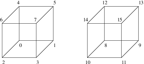
The starting point of our construction is the Kummer lattice which plays an important role in the study of Kummer surfaces. This connection was made clear in [68], and most of this section is based on that work. The Kummer lattice is constructed starting with a set of sixteen orthogonal vectors satisfying . The index set has the structure of a vector space over the finite field 99 9 The set has the structure of a field with addition defined modulo 2 and multiplication defined in the usual way. The vector space is the set of 4-bit sequences, where addition and scalar multiplication are carried out bitwise.. This vector space can be visualized as the vertices of a four-dimensional hypercube and is drawn in Figure 5. A hyperplane in is defined as a subset of that satisfies a linear equation of the form , where and are points on the hypercube. When , we have two limiting cases - when , we have the hyperplane , and when , we have the null set. Except for these two cases, every hyperplane has 8 points. Figure 6 shows some examples of hyperplanes in . Let denote the full set of 32 hyperplanes, including the null set and the set . The Kummer lattice, denoted by , is defined as the set of integer linear combinations of the elements
| (36) |

To discuss the relevance of the Kummer lattice to Kummer surfaces, we first define the Picard lattice of a K3 surface. It is the group of holomorphic line bundles on a K3 surface, where the group operation is the tensor product. A line bundle is specified by its first Chern class which is an element of . A complex structure on induces a Hodge decomposition as discussed in Section 2. Thus, a holomorphic line bundle is specified by an element of . At a general point in the complex structure moduli space, a K3 surface has no holomorphic line bundles. This is because the space is orthogonal to the real 2-plane defined by (holomorphic 2-form) in and in general does not pass through the points of the 22-dimensional integral lattice . The Kummer surface obtained by the blow-up of is very special since it contains sixteen orthogonal holomorphic curves (equivalent to holomorphic line bundles). Thus, the Picard lattice of a Kummer surface contains the lattice spanned by as a sub-lattice. It was shown in [68] that in fact, the Picard lattice of a Kummer surface contains the Kummer lattice as a primitive sub-lattice88 8 If is a K3 surface, then is Kummer The Kummer lattice has a unique, primitive embedding in .
B.3 Construction of a basis for
We now use the notion of primitive embeddings, defined in Section 5.2 and Appendix A, to construct a basis for starting from the Kummer lattice, which is a primitive sub-lattice of . This is an example of “gluing theory”, which is described in some detail in [56]. This approach was used to enumerate all the even, unimodular lattices in 24 dimensions.
Before discussing the case, we consider a simpler example which will serve to illustrate the method. Consider the lattice with as shown in Figure 7. This is an odd, unimodular lattice. The lattice with has a primitive embedding with . Now, the lattice has discriminant . The orthogonal complement is the lattice with disciminant . Thus, we have . The lattice . The quotient is the finite abelian group . The lattice is therefore an overlattice33 3 As discussed in Section 6.2.1 a lattice is an overlattice of a lattice if the lattice has an embedding into , and the quotient is a finite, non-trivial abelian group. of with index 2 (See Figure 7). So if we were to construct the unimodular lattice starting from , we would have to include additional fractional linear combinations of and since . To determine which precise linear combination we must add, notice that . The lattice is an index 2 overlattice of . This leads us to look at the finite abelian group . The lattice is generated by , and to generate a unimodular overlattice we must add one or more elements from to the generating set. Since we want the overlattice to be integral, there is a unique choice — . Recall that . Adding the vector to the generating set gives the unimodular lattice .

Now, we use a similar approach to construct the unimodular lattice starting from and its orthogonal complement , which we denote . This construction has been discussed in [68, 59, 69]. Since is a unimodular lattice and is a primitive sublattice with , the orthogonal complement is an even, signature (3,3) lattice with [59]. The lattice consists of 2-cycles in the Kummer surface that are orthogonal to all the exceptional cycles . From the construction of the Kummer surface , it is clear that these 2-cycles are precisely the cycles that descend from the . As discussed in Appendix A, is an even, signature (3,3) lattice isomorphic to . If we denote the four 1-cycles of by , the six 2-cycles are given by . These 2-cycles satisfy etc. is constructed as the quotient of by the involution. Each 2-cycle in is invariant under this action and under the image of quotient projection, . The lattice spanned by the 2-cycles in the quotient space is isomorphic to . Therefore, and as expected . The lattice is therefore an overlattice of the orthogonal sum of the lattice (toroidal cycles) and the Kummer lattice (exceptional cycles) denoted .
As discussed in the previous example, to generate the even, unimodular overlattice of , we must add to the generators of elements from the quotient . Here denotes the group associated with a lattice . Both abelian groups and have elements since . Since , . It is easy to see that and hence . is generated by the set . The elements of the quotient can be written in terms of two-dimensional planes in the geometry [69] as follows -
| (37) |

The set of two-planes in is obtained by taking all possible intersections of two hyperplanes. Some examples of two-planes are shown in Figure 8. To understand why this is the case, recall that the elements of are maps from to by the action of the inner product. Since , each (non-trivial) element is of the form or else it would map to a non-integer. Also, the point set must not be a hyperplane or which goes to zero in the quotient . Next, we should make sure that the elements of of the form are mapped to integral values by . For this to happen, the point set must intersect every hyperplane in an even number of points. If is a 2-plane in , it is easy to see that this is true. In addition, we must include linear combinations (modulo 1 of course) of these elements giving (37). It can be verified that the group .
Recall from the toy example that we cannot add arbitrary elements of to the generating set of since that would make the lattice non-integral. For example, adding all the generators of would result in the lattice which has determinant . In [68] (stated in this form in [69]) it was shown that given a group isomorphism , the lattice can be constructed as the sub-lattice of as
| (38) |
where are the projections of onto the quotient spaces and respectively. In a sense the isomorphism ensures that only “half” the elements of are added to the generating set thereby making the determinant 1. There is a natural choice for the isomorphism , which is specified by its action on the generators of as
| (39) |
Here is the 2-plane in along the directions . For example,
This construction makes it easy to find an explicit basis for in terms of the toroidal cycles and the exceptional cycles . First, we find a basis for the lattices and . For the Kummer lattice a basis can be found by starting with the basis for a sublattice and then looking for lattice points inside the primitive unit cell. There are 31 such points, given by the “hyperplane vectors,” which are not integer linear combinations of the basis . Choose one such vector and add it to the basis and drop one of the such that the new basis spans a lattice with . This process is repeated until we have a basis for .
To find a basis for , start with a generating set comprising (a) The basis vectors of , (b) the basis vectors of the Kummer lattice obtained by the above procedure, and (c) extra “gluing vectors” of the form , where is the 2-plane spanned by the directions in . It is clear that these vectors generate the unimodular lattice from the construction of in (38). These vectors however are not linearly independent and form an overcomplete basis of . We drop vectors from the basis that lie in the span of other vectors in the basis thereby obtaining a basis for consisting of 22 vectors. We implemented this procedure and obtained the following basis (which is not unique in any sense)
| (40) |
It can be verified that this construction produces an even, unimodular lattice by computing the matrix of inner products. The signature and determinant can be verified to be (3,19) and -1 respectively.
Appendix C Embeddings into Even, Unimodular Lattices
For the construction of magnetized brane models on K3 in this paper, we are interested in embeddings of even lattices in . In the case of embeddings into an even, unimodular lattice, the paper by Nikulin [57] contains two theorems which will be extremely useful. The first theorem, which we quote below, was originally derived by James [71]. The second theorem, derived by Nikulin, strengthens the result by weakening the conditions on the lattice .
Theorem C.1 (James).
Let be an even lattice of signature and let be an even, unimodular lattice of signature . If , then a primitive embedding of into exists. Moreover, this embedding is unique up to an automorphism of .
This theorem is a generalization of the theorem by Wall [54] discussed in Section 5.1. Theorem C.1 can be applied to embeddings of lattices in in a similar manner to the embeddings of vectors discussed in Section 5.1, but breaks down when the rank of is equal to 3 or higher. Nikulin proved a further extension of this theorem which applies for higher rank . We quote Nikulin’s theorem 1.14.4 from [57], using his remark 1.14.5 to simplify the last condition, and with an inequality in the last condition which follows from the other results in the paper and which is presumably implicit in Nikulin’s statement of the theorem.
Theorem C.2.
Let be an even lattice of signature and let be an even, unimodular lattice of signature . There exists a unique primitive embedding of into , provided the following conditions hold:
- 1.
and .
- 2.
.
- 3.
and if equality holds then .
To understand the statement of this theorem, we must define . Given any even lattice , there is an associated finite abelian group called the dual quotient group defined as the quotient . Here denotes the dual lattice of . For every prime the -component of denoted is defined as the subgroup of all elements whose order is a power of . Then, . denotes the number of generators of the -component of . For example, consider the lattice defined as the lattice generated by and with the inner products . The basis for the dual lattice is composed of the elements and defined as
| (41) |
An element is naturally associated with an element in using the inner product. For example, can be regarded as the elements and respectively. Thus the dual lattice can be expressed as the space , with . The quotient space therefore is the finite abelian group where addition is . This is the abelian group and is generated by two elements and . In this case, and for . Using Theorem C.2, this means that the lattice has a unique, primitive embedding in . The lattice has and for , and therefore also has a unique, primitive embedding in .
We can derive a simple, but useful upper bound on the number of generators of . Every finite, abelian group can be decomposed into its -components as ; there is a natural projection which is onto. Therefore, is certainly less than the total number of generators of the group . If the rank of the lattice is , the number of generators of is at most . Since is a signature lattice, Theorem C.2 can be used as long as . This provides a proof of Theorem 5.1 in Section 5.2.
One can derive a different upper bound on . Since , where denotes the cardinality of the group. Therefore the prime factorization of determines the cardinality of each -component, but does not determine the group structure. For example, an abelian group of order 4 is isomorphic to either or and therefore has 2 or 1 generators respectively. For an abelian group of order 36, we have four possibilities - with 4, 3, 3 and 2 generators respectively. The general statement is that if is the highest power of that divides , then the candidate abelian groups for are in one-one correspondence with the set of partitions of . For a fixed cardinality of , the number of generators is maximized when , with . Therefore, given a lattice with inner product matrix , where is the highest power of that divides . This implies , where denotes the greatest integer less than or equal to . Using the relation [56], we can derive the upper bound
| (42) |
References
- (1) M. Bershadsky, C. Vafa and V. Sadov, “D-Branes and Topological Field Theories,” Nucl. Phys. B 463, 420 (1996) arXiv:hep-th/9511222.
- (2) E. Witten, “Small Instantons in String Theory,” Nucl. Phys. B 460, 541 (1996) arXiv:hep-th/9511030.
- (3) M. R. Douglas, “Branes within branes,” arXiv:hep-th/9512077.
- (4) M. B. Green, J. H. Schwarz and P. C. West, “Anomaly Free Chiral Theories In Six-Dimensions,” Nucl. Phys. B 254, 327 (1985).
- (5) C. Bachas, “A Way to break supersymmetry,” arXiv:hep-th/9503030.
- (6)
R. Blumenhagen, L. Goerlich, B. Kors and D. Lust,
“Noncommutative compactifications of type I strings on tori with magnetic
background flux,”
JHEP 0010, 006 (2000)
arXiv:hep-th/0007024.
C. Angelantonj, I. Antoniadis, E. Dudas and A. Sagnotti, “Type-I strings on magnetised orbifolds and brane transmutation,” Phys. Lett. B 489, 223 (2000) arXiv:hep-th/0007090. R. Blumenhagen, L. Goerlich, B. Kors and D. Lust, “Magnetic flux in toroidal type I compactifications,” Fortsch. Phys. 49, 591 (2001) arXiv:hep-th/0010198. - (7)
A. M. Uranga,
“Chiral four-dimensional string compactifications with intersecting
D-branes,”
Class. Quant. Grav. 20, S373 (2003)
arXiv:hep-th/0301032.
E. Kiritsis,
“D-branes in standard model building, gravity and cosmology,”
Fortsch. Phys. 52, 200 (2004)
[Phys. Rept. 421, 105 (2005 ERRAT,429,121-122.2006)]
arXiv:hep-th/0310001.
Blumenhagen + cls
R. Blumenhagen, M. Cvetic, P. Langacker and G. Shiu,
“Toward realistic intersecting D-brane models,”
Ann. Rev. Nucl. Part. Sci. 55, 71 (2005)
arXiv:hep-th/0502005.
R. Blumenhagen, B. Kors, D. Lust and S. Stieberger,
“Four-dimensional String Compactifications with D-Branes, Orientifolds and
Fluxes,”
Phys. Rept. 445, 1 (2007)
arXiv:hep-th/0610327.
F. Marchesano,
“Progress in D-brane model building,”
Fortsch. Phys. 55, 491 (2007)
arXiv:hep-th/0702094.
- (8) R. Blumenhagen, G. Honecker and T. Weigand, “Loop-corrected compactifications of the heterotic string with line bundles,” JHEP 0506, 020 (2005) arXiv:hep-th/0504232.
- (9) G. Honecker, “Massive U(1)s and heterotic five-branes on K3,” Nucl. Phys. B 748, 126 (2006) arXiv:hep-th/0602101.
- (10) G. Honecker and M. Trapletti, “Merging heterotic orbifolds and K3 compactifications with line bundles,” JHEP 0701, 051 (2007) arXiv:hep-th/0612030.
- (11) R. Blumenhagen, L. Gorlich and B. Kors, “Supersymmetric orientifolds in 6D with D-branes at angles,” Nucl. Phys. B 569, 209 (2000) arXiv:hep-th/9908130. R. Blumenhagen, L. Gorlich and B. Kors, “Supersymmetric 4D orientifolds of type IIA with D6-branes at angles,” JHEP 0001, 040 (2000) arXiv:hep-th/9912204. R. Blumenhagen, L. Gorlich and B. Kors, “A new class of supersymmetric orientifolds with D-branes at angles,” arXiv:hep-th/0002146. G. Aldazabal, S. Franco, L. E. Ibanez, R. Rabadan and A. M. Uranga, “Intersecting brane worlds,” JHEP 0102, 047 (2001) arXiv:hep-ph/0011132. G. Aldazabal, S. Franco, L. E. Ibanez, R. Rabadan and A. M. Uranga, “D = 4 chiral string compactifications from intersecting branes,” J. Math. Phys. 42, 3103 (2001) arXiv:hep-th/0011073.
- (12) M. R. Douglas and W. Taylor, “The landscape of intersecting brane models,” JHEP 0701, 031 (2007) arXiv:hep-th/0606109.
- (13) S. Banerjee and A. Sen, “Duality Orbits, Dyon Spectrum and Gauge Theory Limit of Heterotic String Theory on ,” JHEP 0803, 022 (2008) arXiv:0712.0043 [hep-th].
- (14) S. Forste, G. Honecker and R. Schreyer, “Supersymmetric Z(N) x Z(M) orientifolds in 4D with D-branes at angles,” Nucl. Phys. B 593, 127 (2001) arXiv:hep-th/0008250.
- (15) M. Cvetic, G. Shiu and A. M. Uranga, “Three-family supersymmetric standard like models from intersecting brane worlds,” Phys. Rev. Lett. 87, 201801 (2001) arXiv:hep-th/0107143. M. Cvetic, G. Shiu and A. M. Uranga, “Chiral four-dimensional N = 1 supersymmetric type IIA orientifolds from intersecting D6-branes,” Nucl. Phys. B 615, 3 (2001) arXiv:hep-th/0107166.
- (16) D. Cremades, L. E. Ibanez and F. Marchesano, “Yukawa couplings in intersecting D-brane models,” JHEP 0307, 038 (2003) hep-th/0302105.
- (17) M. Cvetic, P. Langacker, T. j. Li and T. Liu, “D6-brane splitting on type IIA orientifolds,” Nucl. Phys. B 709, 241 (2005) hep-th/0407178.
- (18) F. Marchesano and G. Shiu, “MSSM vacua from flux compactifications,” Phys. Rev. D 71, 011701 (2005) hep-th/0408059.
- (19) M. Cvetic, T. Li and T. Liu, “Supersymmetric Pati-Salam models from intersecting D6-branes: A road to the standard model,” Nucl. Phys. B 698, 163 (2004) hep-th/0403061.
- (20) R. Blumenhagen, F. Gmeiner, G. Honecker, D. Lust and T. Weigand, “The statistics of supersymmetric D-brane models,” Nucl. Phys. B 713, 83 (2005) arXiv:hep-th/0411173. F. Gmeiner, R. Blumenhagen, G. Honecker, D. Lust and T. Weigand, “One in a billion: MSSM-like D-brane statistics,” JHEP 0601, 004 (2006) arXiv:hep-th/0510170.
- (21) V. Rosenhaus and W. Taylor, “Diversity in the Tail of the Intersecting Brane Landscape,” JHEP 0906, 073 (2009) arXiv:0905.1951 [hep-th].
- (22) I. V. Melnikov, R. Minasian and S. Theisen, “Heterotic flux backgrounds and their IIA duals,” arXiv:1206.1417 [hep-th].
- (23) M. Grana, “Flux compactifications in string theory: A comprehensive review,” Phys. Rept. 423, 91 (2006) arXiv:hep-th/0509003. M. R. Douglas and S. Kachru, “Flux compactification,” Rev. Mod. Phys. 79, 733 (2007) arXiv:hep-th/0610102. F. Denef, M. R. Douglas and S. Kachru, “Physics of string flux compactifications,” Ann. Rev. Nucl. Part. Sci. 57, 119 (2007) arXiv:hep-th/0701050.
- (24) M. R. Douglas, “The statistics of string/M theory vacua,” JHEP 0305 (2003) 046 hep-th/0303194
- (25) V. Balasubramanian, J. de Boer and A. Naqvi, arXiv:0805.4196 [hep-th].
- (26) K. R. Dienes and M. Lennek, “Correlation Classes on the Landscape: To What Extent is String Theory Predictive?,” arXiv:0809.0036 [hep-th].
- (27) G. L. Kane, P. Kumar and J. Shao, “LHC String Phenomenology,” J. Phys. G 34, 1993 (2007) arXiv:hep-ph/0610038.
- (28) T. P. T. Dijkstra, L. R. Huiszoon and A. N. Schellekens, “Supersymmetric standard model spectra from RCFT orientifolds,” Nucl. Phys. B 710, 3 (2005) hep-th/0411129.
- (29) C. Vafa, “The string landscape and the swampland,” arXiv:hep-th/0509212. N. Arkani-Hamed, L. Motl, A. Nicolis and C. Vafa, “The string landscape, black holes and gravity as the weakest force,” JHEP 0706, 060 (2007) arXiv:hep-th/0601001. H. Ooguri and C. Vafa, “On the geometry of the string landscape and the swampland,” Nucl. Phys. B 766, 21 (2007) arXiv:hep-th/0605264.
- (30) P. S. Aspinwall, “K3 surfaces and string duality,” arXiv:hep-th/9611137.
- (31) M. Kreuzer and H. Skarke, “Complete classification of reflexive polyhedra in four dimensions,” Adv. Theor. Math. Phys. 4, 1209 (2002) arXiv:hep-th/0002240.
- (32) P. Griffiths, J. Harris, “Principles of algebraic geometry”. Wiley, New York, 1978.
- (33) M. Berkooz, R. G. Leigh, J. Polchinski, J. H. Schwarz, N. Seiberg and E. Witten, “Anomalies, Dualities, and Topology of D=6 N=1 Superstring Vacua,” Nucl. Phys. B 475, 115 (1996) arXiv:hep-th/9605184.
- (34) C. Bachas, M. Bianchi, R. Blumenhagen, D. Lust and T. Weigand, “Comments on Orientifolds without Vector Structure,” JHEP 0808, 016 (2008) arXiv:0805.3696 [hep-th].
- (35) J. Polchinski and E. Witten, “Evidence for Heterotic - Type I String Duality,” Nucl. Phys. B 460, 525 (1996) arXiv:hep-th/9510169.
- (36) A. Strominger, “Superstrings with Torsion,” Nucl. Phys. B 274, 253 (1986).
- (37) T. Eguchi, P. B. Gilkey and A. J. Hanson, “Gravitation, Gauge Theories And Differential Geometry,” Phys. Rept. 66, 213 (1980).
- (38) M. B. Green, J. H. Schwarz, E. Witten, “Superstring Theory: Volume II”, Cambridge University Press, 1987
- (39) J. F. Morales, C. A. Scrucca and M. Serone, “Anomalous couplings for D-branes and O-planes,” Nucl. Phys. B 552, 291 (1999) arXiv:hep-th/9812071. B. J. Stefanski, “Gravitational couplings of D-branes and O-planes,” Nucl. Phys. B 548, 275 (1999) arXiv:hep-th/9812088.
- (40) E. Witten, “Global Anomalies In String Theory,” Anomalies, Geometry, and Topology, edited by A. White, World Scientific (1985).
- (41) D. S. Freed, “Determinants, Torsion, And Strings,” Commun. Math. Phys. 107, 483 (1986).
- (42) M. Marino, R. Minasian, G. W. Moore and A. Strominger, “Nonlinear instantons from supersymmetric p-branes,” JHEP 0001, 005 (2000) arXiv:hep-th/9911206.
- (43) A. Strominger, “Yukawa Couplings In Superstring Compactification,” Phys. Rev. Lett. 55, 2547 (1985).
- (44) J. Polchinski, String Theory, Volume II, Cambridge University Press, 1998
- (45) E. Witten, “Heterotic string conformal field theory and A-D-E singularities,” JHEP 0002, 025 (2000) arXiv:hep-th/9909229.
- (46) P. S. Aspinwall and D. R. Morrison, “Point-like instantons on K3 orbifolds,” Nucl. Phys. B 503, 533 (1997) arXiv:hep-th/9705104.
- (47) P. S. Aspinwall, “Point-like instantons and the spin(32)/Z(2) heterotic string,” Nucl. Phys. B 496, 149 (1997) arXiv:hep-th/9612108
- (48) K. A. Intriligator, “RG fixed points in six dimensions via branes at orbifold singularities,” Nucl. Phys. B 496, 177 (1997) arXiv:hep-th/9702038.
- (49) J. D. Blum and K. A. Intriligator, “Consistency conditions for branes at orbifold singularities,” Nucl. Phys. B 506, 223 (1997) arXiv:hep-th/9705030.
- (50) J. D. Blum and K. A. Intriligator, “New phases of string theory and 6d RG fixed points via branes at orbifold singularities,” Nucl. Phys. B 506, 199 (1997) arXiv:hep-th/9705044.
- (51) W. Barth, C. Peters, and A. van de Ven, “Compact Complex Surfaces”, Springer, 1984.
- (52) P. K. Tripathy and S. P. Trivedi, “Compactification with flux on K3 and tori,” JHEP 0303, 028 (2003) arXiv:hep-th/0301139.
- (53) The On-Line Encyclopedia of Integer Sequences, AT&T research, http://www.research.att.com/ njas/sequences/A008350
- (54) C. T. C. Wall, “On the Orthogonal Groups of Unimodular Quadratic Forms,” Math Annalen 147, 328 (1962).
- (55) C. F. Gauss, Disquisitiones Arithmeticae, Fleischer, Leipzig (1801). [English translation, Yale University Press (1966)].
- (56) J. H. Conway and N. J. A. Sloane, Sphere Packings, Lattices and Groups, 3rd edition, Springer (1993).
- (57) V. V. Nikulin, “Integral Symmetric Bilinear Forms and Some of their Applications”, Mathematics of the USSR-Izvestiya, 1980, 14, No. 1, 103-167.
- (58) Dolgachev, Igor, “Integral quadratic forms : applications to algebraic geometry”, Séminaire Bourbaki, 25 (1982-1983), Exposé No. 611, 28 p
- (59) D. R. Morrison, “On K3 surfaces with large Picard number”, Invent. Math. 75 (1984), 105-121
- (60) G. W. Moore, “Arithmetic and attractors,” arXiv:hep-th/9807087.
- (61) William H. Press, Saul A. Teukolsky, William T. Vetterling, and Brian P. Flannery, “Numerical Recipies in C: the art of scientific computing”, Cambridge University Press, 2nd edition, 1992.
- (62) F. Denef and M. R. Douglas, “Computational complexity of the landscape. I,” Annals Phys. 322, 1096 (2007) arXiv:hep-th/0602072.
- (63) M. Cvetic, T. Li and T. Liu, “Supersymmetric Pati-Salam models from intersecting D6-branes: A road to the standard model,” Nucl. Phys. B 698, 163 (2004) arXiv:hep-th/0403061.
- (64) E. G. Gimon and J. Polchinski, “Consistency Conditions for Orientifolds and D-Manifolds,” Phys. Rev. D 54, 1667 (1996) arXiv:hep-th/9601038.
- (65) K. Dasgupta, G. Rajesh and S. Sethi, “M theory, orientifolds and G-flux,” JHEP 9908, 023 (1999) arXiv:hep-th/9908088.
- (66) P. S. Aspinwall and R. Kallosh, “Fixing all moduli for M-theory on K3 x K3,” JHEP 0510, 001 (2005) arXiv:hep-th/0506014.
- (67) J. P. Serre, A Course in Arithmetic, Springer-Verlag, New York, NY, 1973.
- (68) V. V. Nikulin, “On Kummer surfaces”,Mathematics of the USSR-Izvestiya, 1975, 9, 261-275.
- (69) W. Nahm and K. Wendland, “A hiker’s guide to K3: Aspects of N = (4,4) superconformal field theory with central charge c = 6,” Commun. Math. Phys. 216, 85 (2001) arXiv:hep-th/9912067.
- (70) Kumar, A.: K3 Surfaces of High Rank. PhD thesis, Harvard (2006)
- (71) D. G. James, “On Witt’s theorem for unimodular quadratic forms”, Pacific J. Math. 26 (1968), 303-316.