Cosmic microwave background with Brans-Dicke gravity II: constraints with the WMAP and SDSS data

Feng-Quan Wu Email: wufq@bao.ac.cn Affiliation: National Astronomical Observatories, Chinese Academy of Sciences,
20A Datun Road, Chaoyang District, Beijing 100012, China Xuelei Chen Email: xuelei@cosmology.bao.ac.cn Affiliation: National Astronomical Observatories, Chinese Academy of Sciences,
20A Datun Road, Chaoyang District, Beijing 100012, China

August 24, 2026

Abstract

Using the covariant formalism developed in a companion paper [1](paper I), we derive observational constraint on the Brans-Dicke model in a flat Friedmann-Lemaître-Robertson-Walker (FLRW) universe with cosmological constant and cold dark matter. The cosmic microwave background (CMB) observations we use include the Wilkinson Microwave Anisotropy Probe (WMAP) five year data, the Arcminute Cosmology Bolometer Array Receiver (ACBAR) 2007 data, the Cosmic Background Imager (CBI) polarization data, and the Balloon Observations Of Millimetric Extragalactic Radiation and Geophysics (BOOMERanG) 2003 flight data. For the large scale structure (LSS) we use the matter power spectrum data measured with the luminous red galaxy (LRG) survey of the Sloan Digital Sky Survey (SDSS) Data Release 4 (DR4). We parametrize the Brans-Dicke parameter $\omega$ with a new parameter $\zeta=\ln(1/\omega+1)$ , and use the Markov-Chain Monte Carlo (MCMC) method to explore the parameter space. We find that using CMB data alone, one could place some constraint on positive $\zeta$ or $\omega$ , but negative $\zeta$ or $\omega$ could not be constrained effectively. However, with additional large scale structure data, one could break the degeneracy at $\zeta<0$ . The $2\sigma$ (95.5%) bound on $\zeta$ is $-0.00837<\zeta<0.01018$ (corresponding to $\omega<-120.0$ or $\omega>97.8$ ). We also obtained constraint on $\dot{G}/G$ , the rate of change of $G$ at present, as $-1.75\times 10^{-12}{\rm yr}^{-1}<\dot{G}/G<1.05\times 10^{-12}{\rm yr}^{-1}$ , and $\delta G/G$ , the total variation of $G$ since the epoch of recombination, as $-0.083<\delta{G}/G<0.095$ at $2\sigma$ confidence level.

Keywords:

Brans-Dicke theory, alternative gravity, variation of gravitational constant, cosmic microwave background,large scale structure

I Introduction

The Jordan-Fierz-Brans-Dicke theory[2, 3, 4, 5, 6] (hereafter the Brans-Dicke theory for simplicity) is the most natural alternative to the standard general relativity theory and the simplest example of a scalar-tensor theory of gravity[7, 8, 9, 10, 11]. The gravitational constant becomes a function of space and time, and is proportional to the inverse of a scalar field. Its action in the usual (Jordan) frame is

{\mathcal{S}}=\frac{1}{16\pi}\int d^{4}x\sqrt{-g}\left[-\phi R+\frac{\omega}{\phi}g^{\mu\nu}\nabla_{\mu}\phi\nabla_{\nu}\phi\right]+{\mathcal{S}}^{(m)},

(1)

where $\phi$ is the Brans-Dicke field, $\omega$ is a dimensionless parameter, and ${\mathcal{S}}^{(m)}$ is the action for the ordinary matter fields ${\mathcal{S}}^{(m)}=\int d^{4}x\sqrt{-g}{\mathcal{L}}^{(m)}.$ For convenience, we also define a dimensionless field

\varphi=G\phi,

(2)

where $G$ is the Newtonian gravitational constant. The Einstein equations are then generalized to

	$\displaystyle G_{\mu\nu}$	$\displaystyle=$	$\displaystyle\frac{8\pi G}{\varphi}T^{(m)}_{\mu\nu}+\frac{\omega}{\varphi^{2}}(\nabla_{\mu}\varphi\nabla_{\nu}\varphi-\frac{1}{2}g_{\mu\nu}\nabla_{\lambda}\varphi\nabla^{\lambda}\varphi)$		(3)
			$\displaystyle+\frac{1}{\varphi}(\nabla_{\mu}\nabla_{\nu}\varphi-g_{\mu\nu}\nabla_{\lambda}\nabla^{\lambda}\varphi),$		(3)

where $T^{(m)}_{\mu\nu}$ is the stress tensor for all matter except for the Brans-Dicke field, and the equation of motion for $\varphi$ is

\nabla_{a}\nabla^{a}\varphi=\frac{\kappa}{2\omega+3}T^{(m)\mu}_{\mu},

(4)

In order to match the result of Cavendish type experiments, the present day value of $\varphi$ should be

\displaystyle\varphi_{0}=\frac{2\omega+4}{2\omega+3}.

(5)

The original motivation of the Brans-Dicke theory is the idea that the gravitational constant $G$ ought to be related to the average value of a scalar field, which is determined by the mass density of universe, so that the Mach principle is satisfied [5, 6]. Later, it is noted that the scalar-tensor gravity appears in the low-energy limit of supergravity theories from string theory [12] and other higher-dimensional gravity theories [13]. The Brans-Dicke field may be associated with the dilaton-graviton sector of the string effective action [12, 14]. The dimensionless parameters in string theory - including the value of the string coupling constant - can ultimately be traced back to the vacuum expectation values of scalar fields [15].

The unexpected discovery of the accelerating expansion of the Universe [16, 17, 18] forced us to look for an explanation of the so called “dark energy” which may drive such acceleration. Scalar fields rolling down a proper potential may serve as a dynamical dark energy model [19, 20, 21, 22, 23, 24, 25]. However, in these phenomenological models, the scalar fields are added by hand, the connection to fundamental physics is often unclear. The Brans-Dicke field $\phi$ is a natural candidate for the scalar field, this is the so called “extended quintessence” scenario [26, 27, 28, 29, 30, 31, 32]. Alternatively, the Brans-Dicke theory could also serves as an effective model of the $f(R)$ gravity, in which the gravity is invoked to explain the cosmic acceleration [33, 34, 35, 36, 37, 38, 39, 40, 41, 42, 43, 44, 29, 45, 46].

The Brans-Dicke theory is reduced to the Einstein theory in the limit of

\omega\to\infty,\quad\varphi^{\prime}\to 0,\quad\varphi^{\prime\prime}\to 0.

(6)

So in some sense it could never be excluded completely if Einstein’s general relativity theory turns out to be the final words on the classical theory of gravitation. So far, no significant deviation from the Einstein theory has been discovered, and the most stringent limit on the Brans-Dicke theory comes from solar-system experiments which constrain the parametrized post-Newtonian (PPN) parameter $\gamma=(1+\omega)/(2+\omega)$ . A recent significant result was reported in 2003 using the Doppler tracking data of the Cassini spacecraft while it was on its way to Saturn, with $\gamma-1=(2.1\pm 2.3)\times 10^{-5}$ at $2\sigma$ confidence level [47], which corresponds to about $|\omega|>40000$ . The limitation of such experiments is that they are “weak-field” experiments and probe only a very limited range of space and time. They could not reveal spatial or time variation of gravitational constant on larger scales.

It has long been known that cosmological observations such as the cosmic microwave background (CMB) and large scale structure (LSS) could be used to test the Brans-Dicke theory [48, 49, 50, 51, 52, 53, 54, 55, 56, 57, 58, 59]. While the constraints obtainable with such methods are generally weaker than the solar system tests, they probe a much larger range of space and time. In recent years, with the launch of the WMAP satellite, and the completion of the 2dF and SDSS redshift surveys, it is interesting to put such test into practice.

In 2003, Nagata et al. used the WMAP first year data and $\chi^{2}$ test method to derive a constraint on the Brans-Dicke parameter. They obtained $\omega>1000$ at $2\sigma$ confidence level[55]. However, in 2004, Acquaviva et al. obtained a new constraint using a Markov Chain Monte Carlo approach with CMB data from the WMAP first year data, the ACBAR, VSA and CBI data, and the galaxy power spectrum data from 2dF. They obtain a result of $\omega>120$ at $2\sigma$ confidence level[56]. These two limits differ by an order of magnitude. We are unable to reproduce the result of Ref. [55], but we did reproduce successfully the result of Ref. [56] using the procedures described in their paper and the same data set as they used.

Nevertheless, as will be discussed in the next section, there is room for improvement upon the method used in Ref. [56]. Moreover, new CMB and LSS data have since become available, it is therefore time to revisit this problem with a new approach and update the constraint with the latest observational data.

We have developed a covariant and gauge invariant method for calculating the CMB anisotropy in Brans-Dicke theory, the formalism of our approach is presented in the companion paper [1] (paper I). In the present paper, we apply the method developed in paper I, and use the latest CMB data and large scale structure data to constrain the Brans-Dicke parameters. Here we consider only the case of the massless Brans-Dicke model with cold dark matter and cosmological constant. The more interesting case of the Brans-Dicke field with interacting potential would be investigated in future study.

II Methods

The formalism of calculating CMB angular power spectra and matter power spectrum in Brans-Dicke theory with the covariant and gauge invariant method are presented in paper I. We also described in that paper the numerical implementation of the method in the CMB code CAMB [60]. The results of the modified CAMB code have been check with the results given by Chen and Kamionkowski (1999) in Ref.[53], which was based on a modified version of CMBFAST in the synchronous gauge. The output of the two code show excellent agreement. Our new code has been implemented with some techniques to improve the architecture of program, and the code is much faster than the old one. We refer the reader to paper I for more details.

We consider deriving the constraint on the Brans-Dicke model with the observational data using the Markov Chain Monte Carlo (MCMC) simulation. The CAMB code is used by the public COSMOMC code [61] as the driver for calculating the CMB angular power spectra and matter power spectrum. Here we use the modified CAMB code in the COSMOMC simulation.

The data we used to constrain the Brans-Dicke model are the latest cosmic microwave background power spectrum data, which include the WMAP five-year[62], ACBAR 2007[63], CBI polarization[64] and BOOMERanG 2003[65, 66, 67] data. We also use the galaxy clustering power spectrum data derived from the SDSS LRG survey DR4 [68].

We do not use the Type Ia supernovae (SNe Ia) data when making the constraint in this paper, because the value of the gravitational constant varies during the expansion of the Universe. We know that the Chandrasekhar mass $M_{Ch}\propto G^{-3/2}$ . The variation of the gravitational constant $G$ means that the peak luminosity of SNe, which is approximately pproportional to the Chandrasekhar mass, will change, so the supernovae can not be assumed to be standard candles in this model.

Besides the Brans-Dicke parameter, the cosmological parameters explored in our MCMC simulation are { $\Omega_{b}h^{2}$ , $\Omega_{m}h^{2}$ , $\theta$ , $\tau$ , $n_{s}$ , $\log(10^{10}A_{s}),A_{SZ}$ }. $\Omega_{b}h^{2}$ , $\Omega_{m}h^{2}$ are the baryon and matter densities respectively. The $\theta$ parameter represents the ratio between the sound horizon and the angular diameter distance to the last scattering surface, it is used in lieu of the Hubble parameter $h$ since it is less correlated with other parameters. $\tau$ is the optical depth to reionization, $A_{s}$ is the amplitude of primordial superhorizon power spectrum in the curvature perturbation on $0.05\mbox{Mpc}^{-1}$ scale, $n_{s}$ is the scalar spectral index, $A_{SZ}$ characterizes the marginalization factor of Sunyaev-Zel’dovich effect. We only consider the Brans-Dicke model in a flat universe with the cosmological constant as dark energy. We assume flat priors for these parameters, and the allowed ranges of the parameters are wide enough such that further increasing the allowed ranges has no impact on the results.

In any Bayesian approach to error estimate and parameter constraint, the result will depend somewhat on the parametrization and prior. The original Brans-Dicke parameter $\omega$ is inconvenient to use, because it is unbounded, and the Einstein limit appears at $\omega\to\infty$ . Even if one restrict the allowed range of $\omega$ to some finite interval, the large $\omega$ region would be unduly favored, because at such region the difference in CMB and LSS produced by models of different $\omega$ becomes indiscernibly small.

Acquaviva et al. introduced a variable $\ln\xi=\ln[1/(4\omega$ )] in Ref.[56], and set its prior to be uniform in the range $\ln\xi\in[-9,3]$ , corresponding to $\omega\in[0.01,2025.77]$ . The choice of the lower limit of $\ln\xi$ is motivated by the fact that for $\omega>2000$ , visual inspections show that the CMB angular power spectra become insensitive to $\omega$ . This parametrization is workable, but has some drawbacks: firstly, it does not include the negative values of $\omega$ , and secondly, the lower limit of $\ln\xi_{min}=-9$ , while ostensibly a reasonable choice, is nonetheless put in by hand and quite arbitrary. In fact, the $2\sigma$ limit would be sensitive to this artificial choice, because the likelihood is high and almost flat at $\ln\xi<-9$ , so if one varies the lower limit $\ln\xi_{min}$ , the overall normalization of the posterior probability distribution function would be directly affected.

In this paper, we introduce a new parameter which is more convenient to use:

\zeta=\ln(1+\frac{1}{\omega}).

(7)

This parameter has the nice property that $\zeta\to 0$ asymptotes the Einstein gravity, and it is easy to obtain the two-side (i.e. allows negative $\omega$ ) likelihood distribution around $\zeta=0$ . $\zeta\approx 1/\omega$ when $\omega$ is a large number (i.e. very close to Einstein gravity). We set the allowed range as $\zeta\in[-0.014,0.039]$ , which brackets the Einstein gravity case, and corresponding to $\omega\in[-\infty,-71]\cup[25,\infty]$ . There is no arbitrary limit on large $|\omega|$ value, but only limit on small $|\omega|$ value. Outside this range, i.e. $-71<\omega<25$ , our numerical code break down, because the background evolution deviates too much from the standard model. However, as we are looking primarily for small departures from the Einstein gravity, this is not a big concern, and large departures would have been easily detected by other means as well. When making plots of the likelihood, we do taken into account of the range of allowed parameters, so that the probability is properly normalized. Unavoidably, this artificial restriction on parameter range has some effect on the final result, but as long as the final probability distribution is much smaller than the allowed range, it would not fundamentally change our conclusion.

Refer to caption — Figure 1: The one dimensional marginalized likelihood distributions for the parameter $\zeta$ . “WMAP5” denotes WMAP five-year data. “ALL CMB” represents WMAP five year data plus some small scale data and polarization data, i.e. ACBAR 2007[63], CBI polarization[64] and BOOMERanG 2003[65, 66, 67] data. “LSS” means galaxy clustering power spectrum data from SDSS DR4 LRG data.

III Results

III.1 Constraint on Brans-Dicke Theory

The one-dimensional marginalized likelihood distributions for $\zeta$ is shown in Fig.1. The three curves are obtained with the WMAP data alone (magenta dash-dot curve), with all CMB data, i.e. WMAP, ACBAR, CBI and Boomerang data (blue dashed curve), and with all CMB data as well as the LSS data from SDSS LRG survey (red solid curve). Interestingly, using only the CMB data, we find that a negative $\zeta$ is favored. Indeed, the two curves obtained with only the CMB data declines very slowly at $\zeta<0$ , making it difficult to obtain a limit on negative $\zeta$ with them, so we could not easily quote a number for CMB-only constraint. However, with the additional constraint from the large scale structure data, the best fit value of $\zeta$ goes back to the neighborhood of zero, and the likelihood declines rapidly (almost Gaussian) at negative $\zeta$ . This shows that the large-scale structure data play an very important role in constraining the Brans-Dicke gravity.

To understand this result in more detail, we consider three models:

(1) the original best fit minimal 6-parameter $\Lambda$ CDM model with Einstein gravity obtained by the WMAP team using their 5 year CMB data combined with the distance measurement from SN and the Baryon Acoustic Oscillations(BAO) in the distribution of galaxies[69], which is marked as “WMAP $\Lambda$ CDM” in the figure; (2) the best fit Brans-Dicke mode using only WMAP five-year CMB data, which is marked as “WMAP5” in the figure; (3) the best fit Brans-Dicke model using all CMB data as well as the SDSS LRG data, which is marked as “All CMB+LSS” in the figure.

The CMB angular power spectra and linear galaxy power spectra for these models are plotted in Fig.2 and Fig.3 respectively.

As shown in Fig.2, due to parameter degeneracy, the differences between the three curves of CMB are almost indiscernible: for a slightly negative $\zeta$ , the Brans-Dicke model could produce CMB spectra which fits the data very well. However, as shown in Fig.3, the matter power spectra are quite different. The Brans-Dicke model which best-fit the CMB data does not fit the galaxy power spectra very well. To be sure, if one also allow the bias parameter as a free parameter, the fit could be somewhat improved, nevertheless, it still fails compared to the model obtained by fitting both the CMB and LSS data. Thus, we see that the galaxy power spectrum data could play an important role in distinguishing models, even though when used alone its constraining power is relatively weak.

The 95% marginalized bound we derive in this paper is

-0.00837<\zeta<0.01018

(8)

corresponding to

\omega<-120.0~~~~\rm{or}~~~~\omega>97.8

(9)

We note that when comparing this result with that of Ref. [56], one must remember that we have adopted different parametrization and priors. In fact, we have used CMB data with higher precision (WMAP 5 year vs WMAP 3 year), and additionally we also used the LSS data (SDSS) which they did not use. Despite this improvement in data quality, the limit we derived appears to be slightly weaker than theirs, this is due to the different parametrization and prior we used, particularly, we allowed negative $\omega$ which was not considered in Ref. [56].

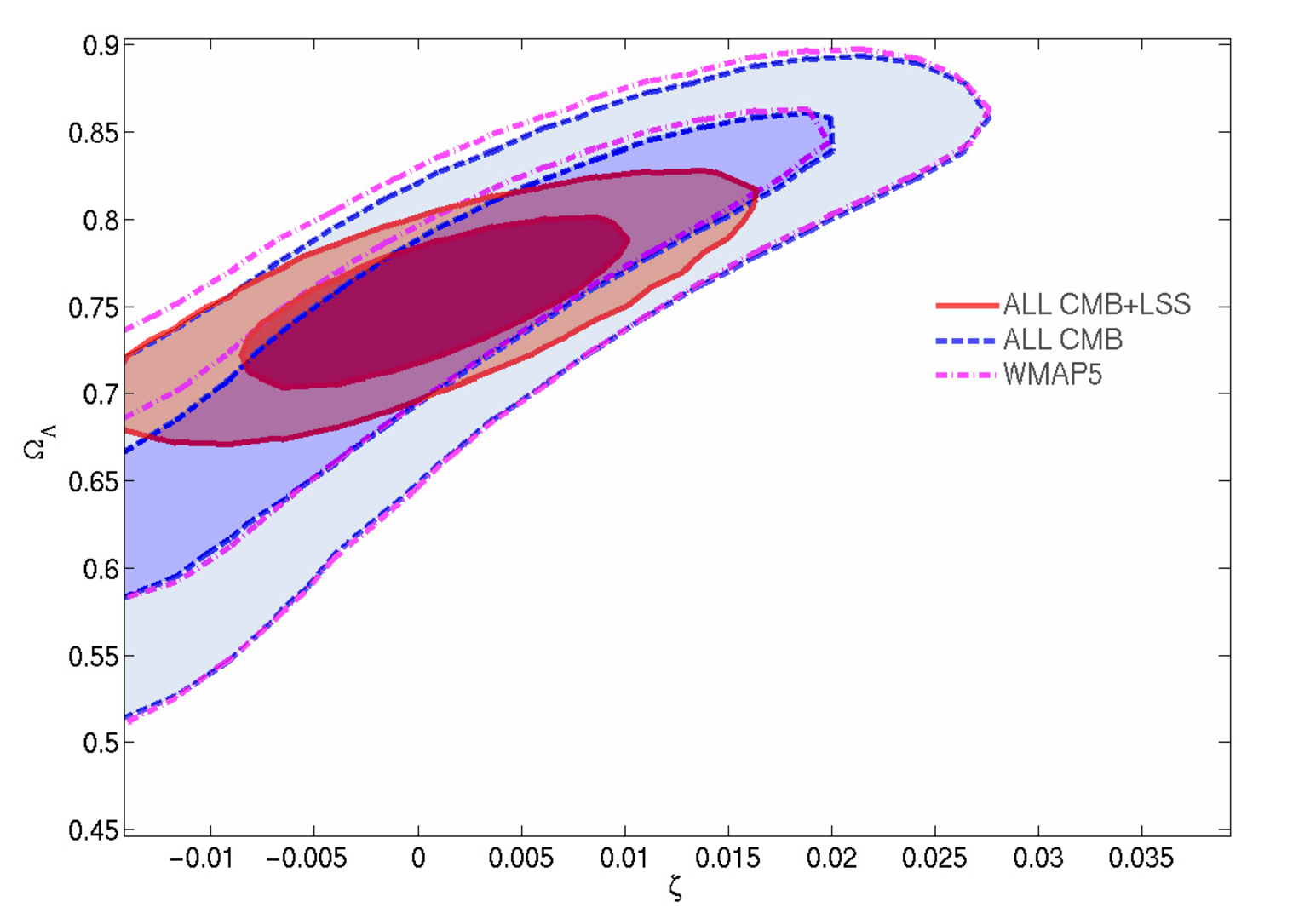
To better understand the degeneracy and the 2-D likelihood space distribution, we plot the 2-D contours of the marginalized likelihood distributions of $\zeta$ against $\Omega_{\Lambda}$ in Fig.4. The Einstein gravity with $\Omega_{\Lambda}\sim 0.75$ is still the best fit model for the all CMB+LSS data set. If $\zeta$ is greater, $\Omega_{\Lambda}$ should also be greater, and vice versa.

III.2 Constraint on cosmological parameters

In Fig.5, we plot one-dimensional marginalized likelihood distributions for other parameters in Brans-Dicke theory(red solid curves), for comparison, we also plot the same distributions in General Relativity case(black dotted curves) which fixes $\xi=0$ , using the same dataset—“ALL CMB+LSS”, i.e. all CMB data combined the LSS data from SDSS LRG survey. The parameters in the top two rows of panels are the primary cosmological parameters used in the MCMC program, and the parameters in the bottom two rows of panels are the derived parameters (not the parameters really run in the MCMC code). We see that the best fit value of the parameters are almost unchanged. Furthermore, for most of the primary parameters, the width of the likelihood distribution is also unchanged. Only the distribution of the dark matter density parameter $\Omega_{c}h^{2}$ is slightly broader. For the derived parameters, the best-fit values are also basically unchanged. However, the likelihood distribution for most parameters are broader, showing the introduction of the Brans-Dicke model allows larger uncertainty in these parameters. The notable exception is the reionization redshift $z_{re}$ which is basically unaffected.

The 2-D contours of of the marginalized likelihood distributions of $\zeta$ against other cosmological parameters are shown in Fig.6. As can be seen in the upper two rows of panels, there are apparently not much correlations between $\zeta$ and the other primary cosmological parameters used in MCMC program, such as $\Omega_{b}h^{2}$ , $\Omega_{m}h^{2}$ , $\theta$ , $\tau$ , $n_{s}$ and $\log(10^{10}A_{s})$ . However, from Fig.4 and the lower two rows of panels of Fig.6, we see that $\zeta$ is correlated with $\Omega_{\Lambda}$ and the derived parameters including the age of Universe, $H_{0}$ , $\Omega_{m}$ , and $\sigma_{8}$ , though there is almost no correlation with the reionization redshift $z_{re}$ .

We summarize the 68% confidence limits on cosmological parameters in Table 1. Note that our pivot wavenumber $k_{0}=0.05~\mbox{Mpc}^{-1}$ of the primordial power spectrum is different from that of the WMAP group 5 year data release ( $k_{0}=0.002~{\rm Mpc^{-1}}$ ), and the set of primary parameters we used is also slightly different from the one used by the WMAP group, as they used $\Omega_{\Lambda}$ instead of $\theta$ as a primary parameter. As we have mentioned, the $\theta$ parameter is less correlated with $\zeta$ , hence our choice in this case could help improve the efficiency of the MCMC method. The data used by the WMAP group [69] are the WMAP five-year data, Type Ia supernovae data and the BAO data. We have not included the supernovae data, which we considered unreliable in the case of modified gravity. From the Table 1, we find that our best-fit values of cosmological parameters are generally consistent with the WMAP group result at one $\sigma$ confidence level, however, our constraints are a bit weaker than those given by the WMAP group, as we have added the Brans-Dicke parameter, and also used somewhat different data sets.

III.3 Constraint on the variation of gravitational constant $G$

An interesting question is what limit could one place on the variation of the gravitational constant $G$ using the CMB and LSS observations. In the Brans-Dicke theory, $G$ also underwent evolution from the time of recombination to the present time, the variation in $G$ is correlated with the value of $\zeta$ , so we can also derive a limit on the variation of the $G$ . Of course, this evolution is not arbitrary, but determined by the dynamical equation Eq. (4), so when citing the bounds on variation of $G$ obtained in this way, one has to remember its limitations. Nevertheless, we note that in the Brans-Dicke theory, the impact on CMB and LSS comes mainly from the variation of $G$ [53, 1], so the result obtained this way could still serve as a good reference value.

Table 1: Summary of cosmological parameters and the corresponding 68% intervals.

Class	Parameter	WMAP5	ALL CMB	ALL CMB+LSS	WMAP group [69]
Primary	$\Omega_{b}h^{2}$	$0.02190_{-0.00062}^{+0.00073}$	$0.02200_{-0.00052}^{+0.00069}$	$0.02229_{-0.00071}^{+0.00033}$	$0.02265\pm 0.00059$
	$\Omega_{c}h^{2}$	$0.1040_{-0.0049}^{+0.0089}$	$0.1064_{-0.0039}^{+0.0077}$	$0.1066_{-0.0046}^{+0.0042}$	$0.1143\pm 0.0034$
	$\theta$	$1.0391_{-0.0024}^{+0.0049}$	$1.0425_{-0.0028}^{+0.0032}$	$1.0432_{-0.0030}^{+0.0018}$
	$\tau$	$0.088_{-0.009}^{+0.009}$	$0.085_{-0.007}^{+0.011}$	$0.093_{-0.014}^{+0.001}$	$0.084\pm 0.016$
	$n_{s}$	$0.947_{-0.006}^{+0.035}$	$0.956_{-0.012}^{+0.027}$	$0.962_{-0.011}^{+0.015}$	$0.960^{+0.014}_{-0.013}$
	$\log[10^{10}A_{s}]$	$3.034_{-0.024}^{+0.074}$	$3.050_{-0.024}^{+0.065}$	$3.070_{-0.047}^{+0.030}$	$A_{s}=(2.457^{+0.092}_{-0.093})\times 10^{-9}$
Derived	$\Omega_{\Lambda}$	$0.780_{-0.009}^{+0.100}$	$0.789_{-0.093}^{+0.076}$	$0.753_{-0.031}^{+0.029}$	$0.721\pm 0.015$
	$\Omega_{b}$				$0.0462\pm 0.0015$
	$\Omega_{c}$				$0.233\pm 0.013$
	Age/Gyr	$14.09_{-1.00}^{+0.97}$	$13.82_{-1.13}^{+0.82}$	$13.63_{-0.44}^{+0.49}$	$13.73\pm 0.12\ \mbox{Gyr}$
	$\Omega_{m}$	$0.210_{-0.085}^{+0.085}$	$0.218_{-0.076}^{+0.093}$	$0.247_{-0.029}^{+0.031}$
	$\sigma_{8}$			$0.789_{-0.055}^{+0.053}$	$0.817\pm 0.026$
	$z_{re}$	$10.4_{-1.5}^{+1.7}$	$10.2_{-1.4}^{+1.8}$	$10.9_{-1.8}^{+0.9}$	$10.8\pm 1.4$
	$H_{0}$	$63.5_{-11.6}^{+12.4}$	$64.4_{-9.7}^{+14.2}$	$72.3_{-4.7}^{+5.0}$	$70.1\pm 1.3$

For making this constraint, we introduce two derived variables in the MCMC, namely the rate of change of the gravitational constant $\dot{G}/G$ at present and the integrated change of gravitational constant since the epoch of recombination $\delta G/G$ :

\dot{G}/G\equiv-\dot{\varphi}/\varphi,\qquad\delta G/G\equiv(G_{rec}-G_{0})/G_{0}.

(10)

The one dimensional marginalized likelihood distributions of $\dot{G}/G$ and $\delta{G}/G$ are plotted in Fig. 7 and Fig. 8 respectively. The “WMAP 5 year data” and the “all CMB data” both favor a slightly non-zero (positive) $\dot{G}/G$ . With the addition of the SDSS power spectrum data, however, the best-fit value is back to zero. From these figures, we could still see some effect of the prior, as the likelihoods are still non-zero or at best just approaching zero at the edge of the figures. Nevertheless, with the LSS data added, the likelihood is quite symmetric around the central value.

With this caveat in mind, we derive the following $2\sigma$ (95.4%) constraints:

-1.75\times 10^{-12}{\rm yr}^{-1}<\dot{G}/G<1.05\times 10^{-12}{\rm yr}^{-1}

(11)

and

-0.083<\delta G/G<0.095

(12)

We also plot 2D contours of marginalized likelihood distributions of $\zeta$ versus $\dot{G}/G$ and $\delta{G}/G$ in Fig. 9 and Fig. 10 respectively. As expected, the variation of gravitational constant is strongly correlated with the value of $\zeta$ in this model.

Some previous constraints on these two variables together with the result of the present paper are summarized in Table 2. We note that in order to obtain such a constraint, one has to make some assumptions, either in the underlying theoretical model, or in the way $G$ varies. This is particularly true for the case of constraints derived from CMB and LSS, as the impact of varying $G$ on these are multitude. For example, Ref.[70] modeled the variations of $G$ by some hypothetical functions, Ref.[71] parametrizes the evolution of $G$ as three forms: constant, linear and Heaviside function, while the present paper assumed Brans-Dicke model. One has to be careful when comparing the different limits, as the assumptions made are often different. Nevertheless, from this table we can get a feeling of the current limits on the variation of gravitational constants.

Table 2: Constraints on the rate of variations of gravitational constant. The errors are

1\sigma

unless otherwise noted.

Parameter	Value	Method	Reference
$\dot{G}/G$	$2\pm 7$	lunar laser ranging	Muller & Biskupek 2007[72]
$[10^{-13}$ yr ${}^{-1}]$	$0\pm 4$	big bang nucleosynthesis	Copi et al. 2004 [73]
			Bambi et al. 2005[74]
	$0\pm 16$	helioseismology	Guenther et al. 1998 [75]
	$-6\pm 20$	neutron star mass	Thorsett 1996 [76]
	$20\pm 40$	Viking lander ranging	Hellings et al. 1983 [77]
	$40\pm 50$	binary pulsar	Kaspi et al. 1994 [78]
	$-96\sim 81~(2\sigma)$	CMB (WMAP3)	Chang & Chu 2007 [70]
	$-17.5\sim 10.5~(2\sigma)$	CMB+LSS	Wu & Chen 2009 (This paper)

IV Conclusion

In this paper, we use the currently available CMB (WMAP five-year[62], ACBAR 2007[63], CBI polarization[64] and BOOMERanG 2003[65, 66, 67]) and the LSS data (galaxy clustering power spectrum from SDSS DR4 LRG data[68]) to constrain the Brans-Dicke theory. We use the covariant and gauge-invariant method developed in paper I to calculate the CMB angular power spectrum and LSS matter power spectrum.

To explore the parameter space, we use the MCMC technique. We parametrize $\omega$ with a new parameter, $\zeta=\ln(1/\omega+1)$ , in order to explore the likelihood distribution of the Brans-Dicke parameter $\omega$ in a continuous interval. This method of parametrization is approximately equivalent to $\zeta=1/\omega$ when $\omega$ is a large number. It allows consideration of negative $\omega$ value, and also there is no arbitrary upper limit on $|\omega|$ (due to numerical problem, one has to choose a lower limit for $|\omega|$ ). We explore in the range $\zeta\in[-0.014,0.039]$ , corresponding to $\omega\in[-\infty,-71]\cup[25,\infty]$ .

We found that while the CMB observation could constrain models with positive $\omega$ , for the present data set and best fit parameter values, there is some degeneracy at $\omega<0$ . The LSS data could effectively remove this degeneracy. Finally, using the CMB and LSS data, we obtain $2\sigma$ (95.5%) limit on $\zeta$ as $-0.00837<\zeta<0.01018$ , corresponding to $\omega<-120.0$ or $\omega>97.8$ . These limits may appear as weaker than previous limit obtained by Ref. [56], even though we used later data than them. However, this difference is largely due to the different assumption made in the constraint. Particularly, we consider case of $\omega<0$ which was not considered in Ref. [56]. As expected, the current limit on $\omega$ derived from CMB and LSS data is much weaker than those derived from solar system tests. However, the large temporal and spatial range probed by these observations make it a useful complementary to the latter.

To examine whether the gravitational coupling is really a constant we introduced two new derived parameters in our MCMC code, one is $\dot{G}/G$ , the rate of change of the gravitational “constant” $G$ at present, and the other is $\delta G/G$ , the integrated change of $G$ since the epoch of recombination. We obtain the $2\sigma$ limit for these two variable as $-1.75\times 10^{-12}{\rm yr}^{-1}<\dot{G}/G<1.05\times 10^{-12}{\rm yr}^{-1}$ and $-0.083<\delta{G}/G<0.095$ respectively. These limits are still somewhat weaker than the solar systems, but again they probed larger scales. Especially for this test, the assumptions made in each technique could be quite different, which one must bear in mind when making comparisons.

The Planck satellite ¹¹ 1 http://www.rssd.esa.int/index.php?project=planck is expect to begin operation and bring back even better CMB data. The SDSS-3 BOSS survey ²² 2 http://cosmology.lbl.gov/BOSS/, http://www.sdss3.org/ , WiggleZ [79], and the LAMOST surveys [80] are expected to measure galaxy power spectrum at higher redshift and with better precision. We look forward to obtain more stringent constraints on the Brans-Dicke theory and other scalar-tensor gravity models in the near future.

Acknowledgements

We thank Antony Lewis, Le Zhang, Yan Gong, Xin Wang, Li’e Qiang, G.F.R. Ellis and Marc Kamionkowski for helpful discussions. X.C. acknowledges the hospitality of the Moore center of theoretical cosmology and physics at Caltech, where part of this research is performed. Our MCMC chain computation was performed on the Supercomputing Center of the Chinese Academy of Sciences and the Shanghai Supercomputing Center. This work is supported by the National Science Foundation of China under the Distinguished Young Scholar Grant 10525314, the Key Project Grant 10533010; by the Chinese Academy of Sciences under grant KJCX3-SYW-N2; and by the Ministry of Science and Technology under the National Basic Science program (project 973) grant 2007CB815401.

References

[1] F.-Q. Wu, L. e Qiang, X. Wang, and X. Chen (2009), eprint 0903.0385.
[2] P. Jordan, Nature (London) 164, 637 (1949).
[3] P. Jordan, Z. Phys. 157, 112 (1959).
[4] M. Fierz, Helv. Phys. Acta 29, 128 (1956).
[5] C. Brans and R. H. Dicke, Phys. Rev. 124, 925 (1961).
[6] R. H. Dicke, Phys. Rev. 125, 2163 (1962).
[7] P. G. Bergmann, Int. J. Theor. Phys. 1, 25 (1968).
[8] J. Nordtvedt, Kenneth, Astrophys. J. 161, 1059 (1970).
[9] R. V. Wagoner, Phys. Rev. D1, 3209 (1970).
[10] J. D. Bekenstein, Phys. Rev. D15, 1458 (1977).
[11] J. D. Bekenstein and A. Meisels, Phys. Rev. D18, 4378 (1978).
[12] M. B. Green, J. Schwarz, and E. Witten, superstring theory (Cambridge University Press, 1987).
[13] T. Appelquist, A. Chodos, and P. Freund, Modern Kaluza-Klein Theories (Addison-Wesley, Redwood City, 1987).
[14] C. A. Clarkson, A. A. Coley, and E. S. D. O’Neill, Phys. Rev. D64, 063510 (2001), eprint gr-qc/0105026.
[15] K. Becker, M. Becker, and J. H. Schwarz, String Theory and M-Theory (Cambridge University Press, 2006).
[16] A. G. Riess et al. (Supernova Search Team), Astron. J. 116, 1009 (1998), eprint astro-ph/9805201.
[17] S. Perlmutter et al. (Supernova Cosmology Project), Nature 391, 51 (1998), eprint astro-ph/9712212.
[18] S. Perlmutter et al. (Supernova Cosmology Project), Astrophys. J. 517, 565 (1999), eprint astro-ph/9812133.
[19] C. Wetterich, Nucl. Phys. B302, 668 (1988).
[20] P. J. E. Peebles and B. Ratra, Astrophys. J. 325, L17 (1988).
[21] J. A. Frieman, C. T. Hill, A. Stebbins, and I. Waga, Phys. Rev. Lett. 75, 2077 (1995), eprint astro-ph/9505060.
[22] M. S. Turner and M. J. White, Phys. Rev. D56, 4439 (1997), eprint astro-ph/9701138.
[23] R. R. Caldwell, R. Dave, and P. J. Steinhardt, Phys. Rev. Lett. 80, 1582 (1998), eprint astro-ph/9708069.
[24] A. R. Liddle and R. J. Scherrer, Phys. Rev. D59, 023509 (1999), eprint astro-ph/9809272.
[25] P. J. Steinhardt, L.-M. Wang, and I. Zlatev, Phys. Rev. D59, 123504 (1999), eprint astro-ph/9812313.
[26] J.-P. Uzan, Phys. Rev. D59, 123510 (1999), eprint gr-qc/9903004.
[27] L. Amendola, Phys. Rev. D60, 043501 (1999), eprint astro-ph/9904120.
[28] T. Chiba, Phys. Rev. D60, 083508 (1999), eprint gr-qc/9903094.
[29] F. Perrotta, C. Baccigalupi, and S. Matarrese, Phys. Rev. D61, 023507 (2000), eprint astro-ph/9906066.
[30] D. J. Holden and D. Wands, Phys. Rev. D61, 043506 (2000), eprint gr-qc/9908026.
[31] C. Baccigalupi, S. Matarrese, and F. Perrotta, Phys. Rev. D62, 123510 (2000), eprint astro-ph/0005543.
[32] X. Chen, R. J. Scherrer, and G. Steigman, Phys. Rev. D63, 123504 (2001), eprint astro-ph/0011531.
[33] S. M. Carroll, V. Duvvuri, M. Trodden, and M. S. Turner, Phys. Rev. D70, 043528 (2004), eprint astro-ph/0306438.
[34] S. Capozziello, Int. J. Mod. Phys. D11, 483 (2002), eprint gr-qc/0201033.
[35] S. Capozziello, S. Carloni, and A. Troisi, Recent Res. Dev. Astron. Astrophys. 1, 625 (2003), eprint astro-ph/0303041.
[36] S. Nojiri and S. D. Odintsov, Phys. Rev. D68, 123512 (2003), eprint hep-th/0307288.
[37] S. Nojiri and S. D. Odintsov, Gen. Rel. Grav. 36, 1765 (2004), eprint hep-th/0308176.
[38] A. D. Dolgov and M. Kawasaki, Phys. Lett. B573, 1 (2003), eprint astro-ph/0307285.
[39] W. Hu and I. Sawicki, Phys. Rev. D76, 064004 (2007), eprint astro-ph/0705.1158.
[40] G. R. Dvali, G. Gabadadze, and M. Porrati, Phys. Lett. B485, 208 (2000), eprint hep-th/0005016.
[41] C. Deffayet, G. R. Dvali, and G. Gabadadze, Phys. Rev. D65, 044023 (2002), eprint astro-ph/0105068.
[42] A. Riazuelo and J.-P. Uzan, Phys. Rev. D66, 023525 (2002), eprint astro-ph/0107386.
[43] G. Esposito-Farese and D. Polarski, Phys. Rev. D63, 063504 (2001), eprint gr-qc/0009034.
[44] N. Bartolo and M. Pietroni, Phys. Rev. D61, 023518 (2000), eprint hep-ph/9908521.
[45] L.-e. Qiang, Y.-g. Ma, M.-x. Han, and D. Yu, Phys. Rev. D71, 061501 (2005), eprint gr-qc/0411066.
[46] S.-F. Wu, G.-H. Yang, and P.-M. Zhang (2008), eprint hep-th/0805.4044.
[47] B. Bertotti, L. Iess, and P. Tortora, Nature 425, 374 (2003).
[48] P. J. E. Peebles and J. T. Yu, Astrophys. J. 162, 815 (1970).
[49] H. Nariai, Prog. Theor. Phys. 42, 742 (1969).
[50] J. P. Baptista, J. C. Fabris, and S. V. B. Goncalves (1996), eprint gr-qc/9603015.
[51] J.-c. Hwang, Class. Quant. Grav. 14, 1981 (1997), eprint gr-qc/9605024.
[52] A. R. Liddle, A. Mazumdar, and J. D. Barrow, Phys. Rev. D58, 027302 (1998), eprint astro-ph/9802133.
[53] X. Chen and M. Kamionkowski, Phys. Rev. D 60, 104036 (1999), eprint astro-ph/9905368.
[54] R. Nagata, T. Chiba, and N. Sugiyama, Phys. Rev. D66, 103510 (2002), eprint astro-ph/0209140.
[55] R. Nagata, T. Chiba, and N. Sugiyama, Phys. Rev. D69, 083512 (2004), eprint astro-ph/0311274.
[56] V. Acquaviva, C. Baccigalupi, S. M. Leach, A. R. Liddle, and F. Perrotta, Phys. Rev. D71, 104025 (2005), eprint astro-ph/0412052.
[57] V. Acquaviva and L. Verde, JCAP 0712, 001 (2007), eprint astro-ph/0709.0082.
[58] C. Schimd, J.-P. Uzan, and A. Riazuelo, Phys. Rev. D71, 083512 (2005), eprint astro-ph/0412120.
[59] S. Tsujikawa, K. Uddin, S. Mizuno, R. Tavakol, and J. Yokoyama, Phys. Rev. D77, 103009 (2008), eprint astro-ph/0803.1106.
[60] A. Lewis and A. Challinor, http://camb.info/ (1999).
[61] A. Lewis and S. Bridle, Phys. Rev. D66, 103511 (2002), eprint astro-ph/0205436.
[62] M. R. Nolta et al. (WMAP), Astrophys. J. Suppl. 180, 296 (2009), eprint astro-ph/0803.0593.
[63] C. L. Reichardt et al. (2008), eprint astro-ph/0801.1491.
[64] J. L. Sievers et al. (2005), eprint astro-ph/0509203.
[65] W. C. Jones et al., Astrophys. J. 647, 823 (2006), eprint astro-ph/0507494.
[66] F. Piacentini et al., Astrophys. J. 647, 833 (2006), eprint astro-ph/0507507.
[67] T. E. Montroy et al., Astrophys. J. 647, 813 (2006), eprint astro-ph/0507514.
[68] M. Tegmark et al. (SDSS), Phys. Rev. D74, 123507 (2006), eprint astro-ph/0608632.
[69] E. Komatsu et al. (WMAP), Astrophys. J. Suppl. 180, 330 (2009), eprint astro-ph/0803.0547.
[70] K.-C. Chang and M. C. Chu, Phys. Rev. D75, 083521 (2007), eprint astro-ph/0611851.
[71] S. Galli, A. Melchiorri, G. F. Smoot, and O. Zahn, Phys. Rev. D80, 023508 (2009), eprint 0905.1808.
[72] J. Muller and L. Biskupek, Class. Quant. Grav. 24, 4533 (2007).
[73] C. J. Copi, A. N. Davis, and L. M. Krauss, Phys. Rev. Lett. 92, 171301 (2004), eprint astro-ph/0311334.
[74] C. Bambi, M. Giannotti, and F. L. Villante, Phys. Rev. D71, 123524 (2005), eprint astro-ph/0503502.
[75] D. B. Guenther, L. M. Krauss, and P. Demarque, Astrophys. J. 498, 871 (1998).
[76] S. E. Thorsett, Phys. Rev. Lett. 77, 1432 (1996), eprint astro-ph/9607003.
[77] R. W. Hellings, P. J. Adams, J. D. Anderson, M. S. Keesey, E. L. Lau, E. M. Standish, V. M. Canuto, and I. Goldman, Physical Review Letters 51, 1609 (1983).
[78] V. M. Kaspi, J. H. Taylor, and M. F. Ryba, Astrophys. J. 428, 713 (1994).
[79] K. Glazebrook et al. (2007), eprint astro-ph/0701876.
[80] X. Wang et al. (2008), eprint astro-ph/0809.3002.