Higgs Boson Exchange Effects in at High Energy
Abstract
We consider the prospects for detecting effects due to the Higgs exchange diagram in high energy , , and collisions producing a pair of bosons. The processes (with ) are analyzed, analytically and via numerical simulations, to determine the center of mass energy, , where the effects from Higgs exchange become relevant. The scaling of with the mass of the incoming leptons is also studied. Special consideration is given to the final state after experimental acceptance cuts are imposed. Angular cuts are shown to be able to significantly lower .
I Introduction
Although the Standard Model (SM) [1, 2, 3] of particle physics is extremely successful in describing elementary particles and their interactions (except gravity), one of the key particles predicted and required by the SM to explain the origin of mass, the so called Higgs boson, still remains elusive. The importance of the Higgs boson in the SM is not limited to the gauge invariant generation of particle masses. For processes like , the coupling of the Higgs boson to fermions and bosons is necessary to maintain S-matrix unitarity. Unitarity of the S-matrix reflects the requirement of probability conservation and requires that partial wave amplitudes behave like () at high energies, , for renormalizable theories [4, 5]. Logarithmically growing terms are also allowed since they may be canceled by higher order corrections [6] and, thus, do not spoil renormalizability.
In 1974, Joglekar [5] showed that S-matrix unitarity forces the couplings of the electroweak gauge bosons and the Higgs boson to take the form of SM couplings at asymptotically high energies. This implies that, for non-zero lepton masses, Higgs boson exchange has to contribute to the process (), and that the coupling of the Higgs boson to leptons and bosons has to be of SM form in order for S-matrix unitarity to be maintained.
In this paper we investigate through analytical calculations and numerical simulations at what center of mass energy, , the Higgs boson exchange diagram in becomes important. In particular we investigate how experimental acceptance cuts on the decay products affect . With linear colliders in the TeV energy range on the drawing board [7, 8], and active development of a muon collider with center of mass energies in the multi-TeV range ongoing [9], the question whether one may be able to detect Higgs boson exchange effects in is of interest.
The remainder of this paper is organized as follows. In Sec. II we discuss in some detail the analytical calculation, and give a brief overview of how our numerical simulations were performed. Results of the numerical simulations are presented in Sec. III. We concentrate on collisions, but also comment on the case, and, for completeness, on the academic case of collisions11 1 collisions are of academic interest only, since the lepton is too short lived for efficient acceleration and collimation into a beam.. We summarize our results in Sec. IV.
II Details of the Numerical and Analytical Calculation
To determine the center of mass energy for which the Higgs exchange diagram becomes important for maintaining S-matrix unitarity in , we calculate the cross section with and without Higgs boson exchange. Including the Higgs boson exchange diagram lowers the total cross section for pair production in lepton collisions. To quantify for which center of mass energy the Higgs exchange diagram becomes relevant, we impose simple requirements which are discussed in more detail below.
If decays are not taken into account, the calculation is simple enough to be carried out analytically. The analytical calculation is presented in Sec. II.1. However, for a more realistic estimate, decays should be taken into account. If both ’s decay leptonically, the final state contains two neutrinos which both escape undetected. This complicates event reconstruction. The small branching ratio of constitutes an additional disadvantage of the all-leptonic final state. If both ’s decay hadronically, the QCD jet process represents a potentially worrisome background. We therefore concentrate on the final state which has a large branching ratio, manageable background, and can be fully reconstructed. To calculate the cross section for , we use the parton level event generator MadEvent [10]. Details of our MadEvent calculation are given in Sec. II.2.
II.1 Analytical Calculation
| -functions |
|---|

Here, and are the momenta of the incoming lepton and anti-lepton, respectively, and and are the momenta of the and bosons. and are the helicities of the and , and and are the polarizations of the bosons. The helicity amplitudes for can be cast in the form [11]
| (2) |
where is the positron charge, , , , is the minimum angular momentum of the system, and is the scattering angle of the with respect to the direction in the center of mass frame. is the conventional -function; its explicit form for is given in Table 1. denotes the remainder of the amplitude.
The explicit expressions for the helicity amplitudes in the high energy limit obtained from the neutrino, photon and exchange diagrams (see Fig. 1) are given by
| (3) |
for transversely polarized bosons with () and ,
| (4) |
for transversely polarized bosons with () and , and
| (5) |
for longitudinally polarized bosons with () and . All other helicity amplitudes are suppressed by a factor or with and, thus, can be ignored in the high energy limit. Furthermore, the kinematic factor softens the amplitudes given by Eqs. (3) and (5), making them numerically smaller than the amplitude given in Eq. (4) for a wide range of scattering angles. In Eqs. (3) – (5), () denotes the mass of the () boson, is the positron charge, and is the weak mixing angle.
When non-zero lepton masses are taken into account, the neutrino diagram produces an extra term which grows proportional to [5] in the high energy limit. This term is canceled by the Higgs exchange diagram. The Higgs exchange amplitude is given by
| (6) |
where ,
| (7) |
is the Yukawa coupling, and are the lepton spinors, is the mass of the Higgs boson, and and are the polarization vectors of the and , respectively. , finally, is the width of the Higgs boson. For the Higgs boson masses currently favored by experimental data [12], . We, therefore, ignore the width of the Higgs boson in the following discussion.
Squaring the amplitude in Eq. (6), averaging over the lepton spins and summing over bosons polarizations results in the following expression
| (8) |
where is the squared center of mass energy. In the high energy limit, the expression in Eq. (8) simplifies to
| (9) |
One can use the expression given in Eq. (9) to estimate . The Higgs exchange diagram becomes important when and the amplitude originating from the remaining three diagrams are of the same order. Since and dominate over a wide range of scattering angles at high energies, we can get a rough idea at what energies the Higgs exchange diagram becomes important by setting Eq. (9) equal to the sum of the squared helicity amplitudes , averaged over the fermion spins, (see Eq. (4)):
| (10) |
where
| (11) |
The center of mass energy for which the Higgs exchange diagram becomes important is then given by
| (12) |
ie. it scales like . Figure 2 shows as a function of the scattering angle . The values for obtained for are listed in Table 2.
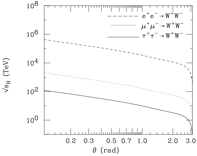 |
| process | (TeV) |
|---|---|
II.2 Simulation of in MadEvent
The results shown in Fig. 2 and Table 2 indicate that Higgs boson exchange becomes relevant at energies much higher than those foreseen for future and colliders. However, these results do not take into account interference effects between the Higgs exchange diagram and the other three diagrams. Furthermore, decays, and effects caused by experimental cuts, are not included.
These effects can easily be taken into account in numerical simulations. We have used the tree-level event generator MadEvent [10] to perform simulations of the process . MadEvent assumes electrons and muons to be massless. Since lepton masses are essential when taking into account the Higgs exchange diagram in , we modified the MadEvent source code to include finite masses for electrons and muons. We only consider the final state. As discussed in Sec. I, the final state can easily be reconstructed, has a fairly large branching ratio, and a relatively small background.
The SM parameters and cuts we used for our simulations are given in Table 3. The Higgs boson mass of GeV was arbitrarily chosen from the accepted Higgs mass range ( GeV at ) [12]. As a quantitative measure for estimating , we require that the cross section with and without Higgs boson exchange differ by a factor 2:
| (13) |
| parameter | value |
|---|---|
| GeV | |
| GeV | |
| GeV | |
| GeV | |
| GeV | |
| GeV | |
| MeV | |
| GeV | |
| GeV | |
| width | GeV |
To simulate detector response, we impose acceptance cuts on the final state particles. For definiteness, we chose cuts similar to those imposed by the LEP experiments [13]. We shall comment below how our results change if these cuts are modified.
It should be noted that the criteria for estimating given in Eqs. (10) and (13) are not identical. In addition to the dominant helicity amplitudes and , Eq. (13) includes the contributions of , and , as well as interference effects between the Higgs exchange amplitude and the other amplitudes. It will be interesting to compare the numerical results obtained using Eq. (10) and (13).
III Numerical Results
 |
 |
We illustrate the effect of the Higgs exchange diagram on the total cross section in Fig. 3 for the case. As expected from the analytic estimate (see Fig. 2), the Higgs exchange diagram becomes important in the few hundred TeV region; Eq. (13) is satisfied for TeV. Similar calculations performed for and collisions also confirm the results of Fig. 2, in particular the scaling of .
The analytic estimate, Eq. (12), gives the center of mass energy as a function of the scattering angle, determined directly from a comparison of the squared amplitudes. Since the squared amplitude is proportional to the differential cross section , it is useful to impose Eq. (13) on the differential cross section, and then compare with the result obtained from Eq. (12). Figure 4 shows for as a function of the center of mass energy with and without Higgs exchange. The dashed lines indicate where the differential cross sections differ by a factor 2.
The analytic estimate for is compared with the result of the MadEvent simulation for , and collisions in Table 4. Although the criteria for obtaining and are somewhat different, the numerical results agree at the 10% level, indicating that the sub-dominant amplitudes and interference effects play a minor role only. In particular, Table 4 confirms that the center of mass energy for which Higgs boson exchange becomes relevant scales with .
| process | (TeV) | (TeV) | percentage difference |
|---|---|---|---|
Comparing Figs. 3 and 4 it is obvious that the Higgs exchange diagram has a more pronounced effect on the differential cross section at larger scattering angles than on the total cross section, which is dominated by the contribution from small values of . This is due to the fact that the Higgs exchange diagram leads to an isotropic distribution of the bosons and their decay products, whereas the contribution from the remaining diagrams is strongly peaked at small scattering angles due to the (massless) neutrino exchange - and -channel diagrams. It also suggests that experimental cuts, in particular angular cuts, could substantially lower the center of mass energy for which Higgs boson exchange becomes important in . To be specific, we impose the following cuts [13] in our subsequent discussion:
| (14) |
Furthermore, the scattering angle of the leptons has to be in the range
| (15) |
and the opening angle between a lepton and a jet has to be . Finally, the invariant mass of the two jets has to be GeV.
Figure 5 shows the cross section, including angular and energy cuts on the final state particles, as a function of the center of mass energy with and without Higgs boson exchange. The center of mass energy for which now is TeV, about a factor 3 less than without cuts.
 |
For () collisions, is larger (smaller) than for collisions. Since the cross section becomes increasingly peaked at smaller scattering angles, and thus at smaller lepton and jet scattering angles, one expects that the angular cuts will lower by a larger (smaller) amount for () collisions. Explicit calculations show that this is indeed the case. Table 5 compares the values of obtained with and without cuts for , , and collisions.
| collisions | (before decays and cuts) | (after decays and cuts) | ratio |
|---|---|---|---|
| TeV | TeV | ||
| TeV | TeV | ||
| TeV | TeV |
The effect of the Higgs exchange diagram can be seen in more detail in the angular distributions of the bosons, and their decay products which are shown for and TeV in Figs. 6 and 7.
 |
 |
| (a) | (b) |
 |
 |
| (a) | (b) |
 |
 |
| (c) | (d) |
The Higgs exchange diagram is seen to have only a small effect at small scattering angles, but becomes much more important for larger values of . For () of the ( scattering angle, the Higgs exchange diagram reduces the differential cross section by almost two orders of magnitude. Because of the V-A nature of the coupling, the decay products inherit the characteristics of the parental differential cross section, i.e. the differential cross sections for the final state neutrino (Fig. 7(a)) and corresponding lepton (Fig. 7(b)) are similar to that of the (see Fig. 6(a)). Most of the final state leptons and neutrinos scatter close to the beam direction. Likewise, for the decaying into two jets, the angular distributions of the jet with maximum transverse energy (Fig. 7(c)) and jet with minimum transverse energy (Fig. 7(d)) are similar to the angular distribution of the (Fig. 6(b)). Because of this similarity between the distributions of the bosons and the final state particles, a relatively larger percentage of the final state particles will scatter close to the beam direction when the Higgs diagram is taken into account than when it is omitted [14]. Thus, imposing experimental acceptance cuts will reduce the differential cross section with the Higgs diagram taken into account by a larger percentage than without.
A more detailed view is offered in Fig. 8, where the pseudorapidity, , of the final state particles is shown for and TeV without imposing any cuts. Here, the pseudorapidity is defined by
| (16) |
 |
 |
| (a) | (b) |
Based on the angular distributions for , we can draw the following conclusions [14]:
- •
The angular cuts imposed on the final state particles remove events where the final state particles scatter close to the beam ( or (). This means that a substantial portion of the total cross section is discarded because of the strong forward peaking of the cross section.
- •
The discarded events constitute a higher percentage of than of due to the fact that most of the cancellations between and occur at large scattering angles. This is a result of the spin 0 nature of the Higgs boson: -channel Higgs exchange leads to an isotropic distribution for the bosons. Due to the character of the coupling, the final state leptons and jets largely inherit the characteristics of the angular distribution of their parents.
- •
Thus, experimental cuts will increase the difference between the and for any particular center of mass energy and shift the values of .
 |
Qualitatively similar results are obtained for and collisions. The results obtained for the cross section with cuts imposed deserve special attention. Fig. 9 shows that the total cross section for the process calculated without the Higgs exchange diagram begins to increase for TeV, which explicitly indicates that S-matrix unitarity is violated.
We now briefly comment on the uncertainties in the simulated data and in the cross section obtained by MadEvent for . Large cancellations between the diagrams result in large uncertainties for both and . At TeV the standard deviation for ab is ab which corresponds to about of the total cross section. For the same center of mass energy, the standard deviation for ab is ab corresponding to of the total cross section. In both cases, the uncertainties in the cross section are large, due to cancellations between the individually divergent amplitudes and . The uncertainties for electron and -lepton collisions are similar.
Finally, we briefly comment on how higher order radiative corrections may affect our results. The full NLO electroweak corrections to including lepton mass effects (and the Higgs exchange diagram) have not been calculated yet. The complexity of the NLO electroweak corrections does not allow us to make educated guesses about the possible effect of these corrections on . However, at high energies, higher order electroweak corrections are known to grow as [15], and eventually have to be resummed. This may considerably change the numerical results presented here. The energy for which Higgs exchange becomes relevant may well increase or decrease by a factor of 2 or more once these effects are taken into account.
IV Summary and Conclusions
In this paper, we have considered the high energy limit of the processes () in order to determine the center of mass energy, , for which the Higgs exchange diagram becomes relevant. In the SM, the Higgs exchange diagram is needed in order to guarantee that S-matrix unitarity is maintained in the high energy limit. Two, slightly different, criteria were used to estimate , both leading to similar results.
From a simplified analytical calculation we found that is of order , where is the mass of the incoming lepton. As a result, the center of mass energies for which Higgs boson exchange becomes important for , and collisions are in the region of TeV), which is far above the energy range of any or collider currently on the drawing board.
We also investigated how experimental acceptance cuts influence the center of mass energy for which Higgs boson exchange becomes important. The - and -channel fermion exchange diagrams result in a strong peaking of the cross section at small scattering angles, which, due to the nature of the -fermion coupling, is inherited by the decay products. The Higgs exchange diagram, on the other hand, leads to a distribution which peaks at large scattering angles. Imposing angular cuts on the final state particles thus tends to lower the center of mass energy for which the Higgs exchange diagram becomes important. The effect of the angular cuts increases with growing energies, and is most pronounced for collisions where the angular cuts chosen in this paper decrease by almost a factor 7. For comparison, for () collisions, angular cuts decrease by about a factor 3 (2.5). For more (less) stringent angular cuts, the effect on increases (decreases).
Our results were obtained from simple tree level calculations and one does have to worry about how higher order electroweak corrections may affect them. Unfortunately, the NLO electroweak corrections to fermions have been computed in the limit of massless incoming leptons only [16]. However, electroweak radiative corrections are known to increase logarithmically with the center of mass energy [15], and, eventually, have to be resummed. They may thus substantially change , although the general order of magnitude estimate presented in this paper should remain correct.
Acknowledgements.
We would like to thank C. Quigg for suggesting the problem. One of us would like to thank the Fermilab Theory Group and the Physics Department, Michigan State University, where part of this work was done, for their generous hospitality. This research was supported by the National Science Foundation under grants No. PHY-0456681 and PHY-0757691.Bibliography
- [1] S. Weinberg, Phys. Rev. Lett. 19, 1264 (1967).
- [2] A. Salam, Originally printed in *Svartholm: Elementary Particle Theory, Proceedings Of The Nobel Symposium Held 1968 At Lerum, Sweden*, Stockholm 367-377 (1968).
- [3] S. L. Glashow, Nucl. Phys. 22, 578-588 (1961).
- [4] C. H. Llewellyn Smith, Phys. Lett. B 46, 233 (1973).
- [5] S. D. Joglekar, Ann. Phys. 83, 427 (1974).
- [6] J. M. Cornwall, D. N. Levin and G. Tiktopoulos, Phys. Rev. D 10, 4, 1145-1167 (1974).
- [7] J. Brau et al., “International Linear Collider reference design report. 1: Executive summary. 2: Physics at the ILC. 3: Accelerator. 4: Detectors,” SLAC-R-857.
- [8] H. Braun et al. [CLIC Study Team Collaboration], CERN-OPEN-2008-021, CLIC-NOTE-764.
- [9] C. Ankenbrandt et al., FERMILAB-TM-2399-APC.
- [10] F. Maltoni and T. Stelzer, JHEP 0302, 027 (2003).
- [11] K. Hagiwara, R. D. Peccei, D. Zeppenfeld, and K. Hikasa, Nucl. Phys. B282, 253 (1987).
- [12] The LEP Collaborations, the LEP Electroweak Working Group, the Tevatron Electroweak Working Group, and the SLD electroweak and heavy flavor working groups, arXiv:0811.4682 [hep-ex].
- [13] D. Bardin et al., arXiv:hep-ph/9709270.
- [14] E. Brewer, PhD Thesis (University at Buffalo), (2008).
- [15] M. Kuroda, G. Moultaka and D. Schildknecht, Nucl. Phys. B 350, 25 (1991); G. Degrassi and A. Sirlin, Phys. Rev. D 46, 3104 (1992); A. Denner, S. Dittmaier and R. Schuster, Nucl. Phys. B 452, 80 (1995) [arXiv:hep-ph/9503442]; A. Denner, S. Dittmaier and T. Hahn, Phys. Rev. D 56, 117 (1997) [arXiv:hep-ph/9612390]; A. Denner and T. Hahn, Nucl. Phys. B 525, 27 (1998) [arXiv:hep-ph/9711302]; M. Beccaria, G. Montagna, F. Piccinini, F. M. Renard and C. Verzegnassi, Phys. Rev. D 58, 093014 (1998) [arXiv:hep-ph/9805250]; P. Ciafaloni and D. Comelli, Phys. Lett. B 446, 278 (1999) [arXiv:hep-ph/9809321].
- [16] A. Denner, S. Dittmaier, M. Roth, and D. Wackeroth, Eur. Phys. J. direct C2, 4 (2000).