Measuring the Higgs boson mass in dileptonic -boson decays at hadron colliders
Abstract
It is expected that hadron collider measurements of the Higgs boson mass using the decay followed by the leptonic decay of each -boson, will be performed by fitting the shape of a distribution that is sensitive to the Higgs mass. We demonstrate that the variable most commonly used to measure the Higgs mass in this channel is not optimal as it contains an unnecessary and even counter-productive approximation. We remove that approximation, without introducing any cost in complexity, and demonstrate that the new variable is a clear improvement over the old: its performance is never worse, and in some cases (particularly the high Higgs mass region) it might reduce the fit uncertainty on the Higgs mass in that channel by a factor approaching two.
.1 Introduction
The mass of the Higgs boson is the last unknown parameter of the Standard Model. Here, we present a method to measure it at a hadron collider, assuming the Higgs exists and is sufficiently massive () that it decays predominantly to -bosons. The method is based on the transverse mass observable, , that was originally used to measure the masses of the -bosons themselves, via their decays, , to a lepton and a neutrino. There, since the neutrino is invisible in a detector, one cannot simply reconstruct the mass of the parent from the invariant mass of the daughter system; the transverse mass circumvents this problem. Similarly, in the case of Higgs decays to two s (one or more of which may be significantly off-mass-shell), then if the s subsequently decay leptonically to , we end up with two invisible neutrinos in the final state. We will describe a generalization of whose distribution features an edge, which will enable us to extract directly. We believe that the method both complements, and improves upon, existing strategies [1, 2, 3] for measuring in this channel, and we encourage experiments to make use of it. The distribution should also aid ongoing Higgs searches at the Tevatron [4, 5].
We also briefly discuss potential applications to mass measurement of other particles at the LHC, for example new resonances (such as Kaluza-Klein gluons from an extra dimension) that decay to , as well as the lightest stable superpartner (LSP) in supersymmetric theories.
The original application of the transverse mass was in measurement of [6, 7, 8]. We define
| (1) |
where is the momentum transverse to the beam, denotes the transverse energy, and and label the visible and invisible decay products respectively, (a charged lepton and a neutrino in the case at hand).
This definition of has two desirable features: first, since the mass of the neutrino is unknown, but negligible, and the transverse momentum of the neutrino can be inferred from the missing transverse momentum in the event, is indeed an observable; second, is always bounded above by the mass of the parent . This is easily shown using the invariant mass constraint
| (2) |
where is the longitudinal momentum and is the energy, together with the lemma
| (3) |
with equality at , which the reader may easily prove for himself. Thus, by computing the distribution of in many events, appears as the upper endpoint. (In practice, the finite decay width of the and other effects lead to appearing as a Jacobian peak in the data.)
Recently, a number of generalizations of have appeared [9, 10, 11, 12, 13, 14, 15, 16, 17, 18], with diverse applications for LHC mass measurements. They include generalizations to: decays with multiple visible daughters; decays with a massive invisible daughter (such as a DM candidate); and decays of pair-produced parent particles. The last of these has already been used to measure the mass of the top quark in the process at the Tevatron [19].
.2 More Invisibles
There is one other generalization that can be made, which is to situations where a single decay in itself contains more than one invisible daughter. Practical examples include the single Higgs decay , the decay of new resonances (such as a Kaluza-Klein gluon) to , followed by a semi-leptonic decay of each top, , or pair decays in supersymmetric theories with both the lightest superpartner and neutrinos in the final state. To generalize to such a situation, the obvious thing to do is to replace in (1) by the invariant mass of the invisible system [20]. Now, in any event, goes unobserved, but it is useful nevertheless to consider its properties. A first observation is that , though a relativistic invariant, now varies from event to event, taking values on some real, positive interval. The endpoints of this interval, , are fixed by the particular decay topology. For example, if a parent of mass undergoes a pointlike three-body decay to one visible particle of mass and two massless invisible particles, the lower and upper endpoints are given by and , respectively, whereas if the decay involves an intermediate resonance of mass , they are given by and .
What is more, it is easy to show that is a monotonically increasing function of . We thus have the chain of inequalities
| (4) |
If is known, then is an observable that is bounded above by ; if is unknown, we can determine it using a generalization of the kink method described in [12, 13, 14, 15].
.2.1 Higgs Decays
For the Higgs decay , it is simple enough to show that , when we ignore the mass of the neutrinos. To wit, consider the on-shell decay , with at rest in the laboratory, in which the two s are emitted back-to-back. Then let the two s decay such that the neutrinos are emitted parallel to each other (not anti-parallel). In this configuration, . Since is positive semi-definite, . Similar arguments apply to the off-shell decay .
That the inequalities in (4) can be made into equalities also follows from the existence of these kinematic configurations. Thus, by computing
| (5) |
in many events, we should obtain a distribution in whose endpoint yields the mass of the Higgs boson. Since the observable defined in (5) is truly bounded above by , we distinguish it from other transverse-mass-like observables by giving it the label .
In work to date [21, 22, 1], an alternative transverse mass has been used,
| (6) |
The justification for replacing the unknown by the observable in those papers is that for Higgs bosons with masses close to and produced at or near threshold, each boson will decay almost at rest, therefore . We note though that is not bounded above by . Not knowing and without using the above approximation, the best lower limit we can place on will be with the true transverse mass (5).
.2.2 simulation
To investigate the relative performance of the alternative transverse mass variables (5) and (6) we use the HERWIG 6.505 [23, 24] Monte Carlo generator, with LHC beam conditions (). Our version of the generator includes the fix to the spin correlations described in [25]. Our simulations do not include all corrections from higher orders in (see e.g. [26] for a comparison). These will be important to consider when later comparing against real experimental distributions.
We generate unweighted events for Standard Model Higgs boson production () and for the dominant background, .11 1 Other backgrounds, such as , are rendered sub-dominant by the cuts discussed below [1]. Final state hadrons with GeV and pseudorapidity are clustered into jets using the longitudinally invariant clustering algorithm for hadron-hadron collisions [27] in the inclusive mode [28] with . The missing transverse momentum is calculated from the vector sum of the transverse momenta of the neutrinos. No detector simulation is applied in this paper. Detector effects should provide a relatively small correction since lepton momenta are very well measured at these energies [1, 2], and the dominant contribution to the missing transverse momentum will be from recoil against well-measured leptons. There will be some additional smearing of from mismeasured and out-of-acceptance hadrons but such corrections are small when the hadronic transverse energy in the event is small [1].
Selection cuts are applied based on [1], requiring:
- •
Exactly two leptons with GeV and
- •
Missing transverse momentum, GeV
- •
- •
No jet with GeV
- •
rejection: the event was rejected if and for both 22 2 The variable is the momentum fraction of the th tau carried by its daughter lepton and is the di-tau invariant mass. They are calculated using the approximation that each was collinear with its daughter lepton.
- •
Relative azimuth
- •
Transverse momentum of the pair system,
As has been done in previous studies [1], we optimize the values of the latter two cuts, and for each Higgs boson mass. In this case we select the values which would be predicted to best constrain – experimentally one would select cuts which would give the best expected measurement once an approximate Higgs boson mass was known. The optimal values ranged from 1.4 to 2.4 for and 0 to 10 GeV for .


Both observables correlate with (see Figure 1), so it is possible to make a mass measurement with either. However does not provide a strict event-by-event lower bound on , whereas the kinematic endpoint of the distribution shows a clear edge at .
To examine the relative performance of the two variables, we generate distributions of them for various choices of . This is done for twenty independent pseudo-experiments (including both signal and the dominant background contributions), each corresponding to integrated luminosity of 10 . Each pseudo-experiment is compared to (signal and background) model distributions with differing hypotheses of .
An example pseudo-experiment distribution for is shown in Figure 2. For each pseudo-experiment the binned log likelihood of the data is calculated. Each likelihood is maximised over the normalisations of the model signal and background distributions, reflecting our uncertainty in the cross-sections and luminosity33 3 While uncertainties in the shapes of these distributions are also likely to be important, they are difficult to estimate without collision data and so are not considered in this paper. We note that shape effects are likely to be more detrimental for ; the position of the kinematic edge in should be robust against uncertainties in smoothly-varying background parameters.:
where the sum is over histogram bins, is the Poisson likelihood and is the expected number of events if signal and background cross sections are times their leading-order Monte Carlo predictions. The angle brackets indicate an average over the twenty pseudo-experiments.
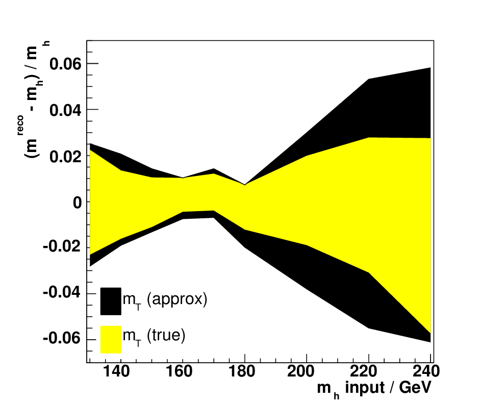
The resulting curves of are plotted in Figure 3, where indicates the difference from the minimum value. The relative precision with which each method can be expected to measure the Higgs boson mass is determined from a quadratic fit to around the minimum. The fractional uncertainties (Figure 4) show that the true transverse mass performs somewhat better than the approximate version for all , so there appears to be no advantage in making the approximation . When there is a significant penalty to pay for assuming — the true transverse mass provides the higher-precision measurement.
The absolute uncertainties (for both variables) will obviously be somewhat broadened when experimental resolution and sub-leading backgrounds are included. While such detailed simulations are beyond the scope of this paper, we project that the desirable properties of will mean it is also the more appropriate variable in the real world.
One might also expect to be a good selection variable for Higgs boson discovery and for measuring the product of cross-section and branching ratio for Higgs production and di-leptonic decay, by counting the number of signal events. Indeed, as discussed in the Appendix, we find that again gives an improvement, albeit a slight one, over in both cases.
.2.3 Other Applications
There are many other possible decay processes at the LHC involving multiple invisible daughters, to which similar methods might be applied. One is to decays of new resonances, such as a Kaluza-Klein gluon from an extra dimension [29], in the channel, followed by semi-leptonic decays of the tops. For heavy resonances (existing constraints suggest that a KK gluon should be multi-TeV, for example), the approximation will certainly be inappropriate.
.3 Conclusions
There seems to be no advantage in using the approximate version of the transverse mass – whether for Higgs boson discovery, for mass determination or for measuring event rates. Indeed our simulations show that the approximation is often counter-productive, particularly if the objective is to make a Higgs boson mass measurement and especially when . The true transverse mass is easy to calculate, and (unlike the approximate version) provides an event-by-event lower bound on .
These results should be cross-checked with more detailed studies with: full detector simulation; more sophisticated models for the signal and background distribution shape uncertainties; and with calculations to higher orders in .44 4 A subsequent study with full detector simulation [30] confirms our results and, in addition, suggests that the true transverse mass appears to have the advantage over of being less correlated with . Future work should also consider the case of Higgs boson production via vector boson fusion for which one might expect rather similar results.
Other examples of processes where this generalization of could be used include Kaluza-Klein gluon decays , where the top quarks decay via leptonic bosons, and supersymmetric decays involving neutrinos, such as .
Although we have focussed our attention here on the decay , it is worth remarking that, in the case of an Standard Model Higgs boson with , the decay channel will allow the Higgs mass to be measured at the per mille level. Nevertheless, the decay would provide an important corroborative measurement.
Acknowledgements.
We are grateful to Bryan Webber for making us aware of [25], to other members of the Cambridge Supersymmetry Working Group, and also to Alessandro Nisati, Bruce Mellado, Bill Quayle and a referee for additional helpful comments. AJB thanks Chris Hays and members of the Oxford Dalitz Institute for useful discussions. This work was supported by the Science and Technology Research Council of the United Kingdom..4 Appendix: Higgs discovery and branching ratio

To quantify the Higgs boson discovery potential using as a selection variable, we calculate the log likelihood difference
where is the likelihood of the trial data when the model contains no Higgs boson contribution. is maximised over , and ; is maximised over .
Plots of this are shown as a function of in Figure 5. The absolute numbers are optimistic, since the discovery potential will be reduced by subdominant backgrounds and detector resolution, but the relative performance of the two variables is meaningful. One can see that the plots are rather similar, but there may be a small advantage in using rather than when .
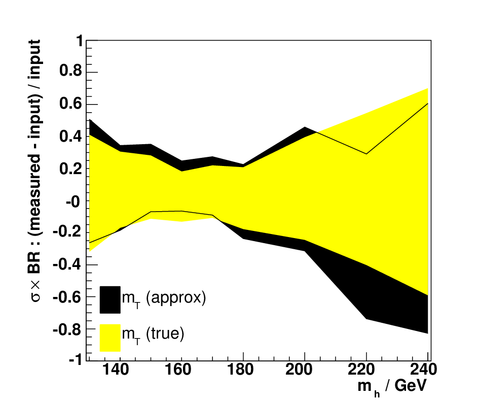
The branching ratio of the Higgs boson to boson pairs is another parameter of significant interest. The relative precision with which one could measure the number of signal events, which is proportional to , was determined from quadratic fits to
for various . The resulting fractional uncertainty bands are shown in Figure 6. There is again an advantage in using , though in this case it is slight.
References
- [1] G. Aad et al. (ATLAS collaboration) (2009), eprint 0901.0512.
- [2] CMS physics technical design report, volume II (2006), CERN-LHCC-2006-021, CMS-TDR-008-2.
- [3] Search strategy for a standard model Higgs boson decaying to two W bosons in the fully leptonic final state (2008), CMS PAS HIG-08-006.
- [4] Search for production at CDF using of data (2009a), CDF note 9500.
- [5] Search for the Higgs boson in decays with at D0 in run II (2009), D0 note 5757.
- [6] G. Arnison et al. (UA1), Phys. Lett. B122, 103 (1983a).
- [7] G. Arnison et al. (UA1), Phys. Lett. B129, 273 (1983b).
- [8] M. Banner et al. (UA2), Phys. Lett. B122, 476 (1983).
- [9] C. G. Lester and D. J. Summers, Phys. Lett. B463, 99 (1999), eprint hep-ph/9906349.
- [10] A. Barr, C. Lester, and P. Stephens, J. Phys. G29, 2343 (2003a), eprint hep-ph/0304226.
- [11] C. Lester and A. Barr, JHEP 12, 102 (2007), eprint 0708.1028.
- [12] W. S. Cho, K. Choi, Y. G. Kim, and C. B. Park, Phys. Rev. Lett. 100, 171801 (2008a), eprint 0709.0288.
- [13] B. Gripaios, JHEP 02, 053 (2008), eprint 0709.2740.
- [14] A. J. Barr, B. Gripaios, and C. G. Lester, JHEP 02, 014 (2008), eprint 0711.4008.
- [15] W. S. Cho, K. Choi, Y. G. Kim, and C. B. Park, JHEP 02, 035 (2008b), eprint 0711.4526.
- [16] D. R. Tovey, JHEP 04, 034 (2008), eprint 0802.2879.
- [17] M. Serna, JHEP 06, 004 (2008), eprint 0804.3344.
- [18] M. Burns, K. Kong, K. T. Matchev, and M. Park (2008), eprint 0810.5576.
- [19] Simultaneous template-based top quark mass measurement in the lepton+jets and dilepton channels using of CDF data (2009b), CDF note 9769.
- [20] A. J. Barr, C. G. Lester, M. A. Parker, B. C. Allanach, and P. Richardson, JHEP 03, 045 (2003b), eprint hep-ph/0208214.
- [21] D. L. Rainwater and D. Zeppenfeld, Phys. Rev. D60, 113004 (1999), eprint hep-ph/9906218.
- [22] S. Asai et al., Eur. Phys. J. C32S2, 19 (2004), eprint hep-ph/0402254.
- [23] G. Corcella et al. (2002), eprint hep-ph/0210213.
- [24] G. Marchesini et al., Comput. Phys. Commun. 67, 465 (1992).
- [25] URL http://projects.hepforge.org/fherwig/trac/ticket/37.
- [26] C. Anastasiou, G. Dissertori, F. Stockli, and B. R. Webber, JHEP 03, 017 (2008), eprint 0801.2682.
- [27] S. Catani, Y. L. Dokshitzer, M. H. Seymour, and B. R. Webber, Nucl. Phys. B406, 187 (1993).
- [28] S. D. Ellis and D. E. Soper, Phys. Rev. D48, 3160 (1993), eprint hep-ph/9305266.
- [29] K. Agashe, A. Delgado, M. J. May, and R. Sundrum, JHEP 08, 050 (2003), eprint hep-ph/0308036.
- [30] W. B. Quayle, private communication.