Error Threshold for Color Codes and Random 3-Body Ising Models

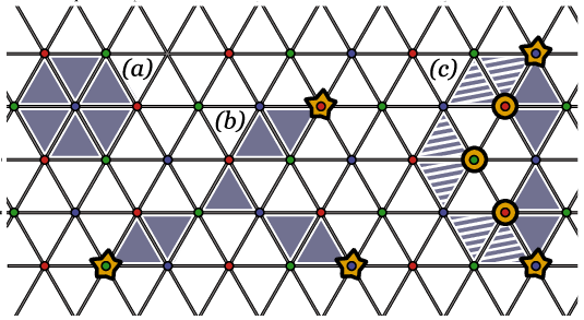
To construct a TCC ${\cal C}$ we start from any two-dimensional (2D) lattice in which all plaquettes are triangles and vertices are 3-colorable, such that no link connects vertices of the same color. The lattice is embedded in a compact surface of arbitrary topology. Since information is encoded in topological degrees of freedom, the code is nontrivial only when the topology of the surface is nontrivial, e.g., a torus of genus $g\geq 1$. So far, color codes have been introduced in the dual lattice (2-colex [11]). Here we prefer to work in the triangular lattice to have a more direct mapping, see Fig. 2.

We consider a physical system with a qubit at each lattice triangle, and introduce the following vertex operators that generate the stabilizer group of $\mathcal{C}$. For each vertex $v$ we have two types of operators which correspond to Pauli operators of $X$ or $Z$ type, i.e., $X_{v}:=\bigotimes_{\triangle:v\in\triangle}X_{\triangle}$ and $Z_{v}:=\bigotimes_{\triangle:v\in\triangle}Z_{\triangle}$. Thus, a vertex operator acts on all nearby triangles, see Fig. 2. Vertex operators pairwise commute and square to identity. The code $\mathcal{C}$ is defined as the subspace with $X_{v}=Z_{v}=1\;\forall v$. To perform error correction one measures vertex operators. The resulting collection of $\pm 1$ eigenvalues is the error syndrome.

Color codes have a structure with stabilizer generators which are either products of $X$ or $Z$ Pauli operators, but not both. This allows us to treat bit-flip and phase errors separately, making the procedure classical: $X$-type ($Z$-type) errors produce violations of $Z$-type ($X$-type) vertex operators. Without loss of generality, let us consider the bit-flip case, that is, errors of the form $X_{E}:=\bigotimes_{\triangle\in E}X_{\triangle}$, where $E$ is the subset of triangles that suffered a bit-flip. Let $\partial E$ be the collection of vertices that are part of an odd number of triangles in $E$, i.e., the boundary of a set of triangles $E$ is chosen so that the error $X_{E}$ gives rise to a syndrome with $Z_{v}=-1$ at those vertices $v\in\partial E$, see Fig. 2. In trying to correct the error, we apply to the system bit-flips $X_{E^{\prime}}$ with the same boundary, $\partial E^{\prime}=\partial E$. This is only successful as long as $X_{E^{\prime}}X_{E}=:X_{E+E^{\prime}}$ is an element of the stabilizer group. Geometrically, $D=E+E^{\prime}$ is a cycle: its boundary $\partial D$ is empty. Given a vertex $v$, let $\partial v$ be the subset of triangles meeting at $v$. We say that $D$ is a boundary if $D=\sum_{V}\partial v$ for some subset of triangles $V$. In that case, $X_{D}$ is an element of the stabilizer group. Thus, error correction is successful whenever $D$ is a boundary, i.e., if $D$ has trivial homology. In that case the real error $E$ and the guessed error $E^{\prime}$ belong to the same homology class.

We consider a standard error model based on stochastic errors in which phase errors $Z$ and qubit bit-flip errors $X$ are uncorrelated and occur with probability $p$ at each qubit. We focus on the correction of bit-flip errors.

Let $P(E)$ be the probability for a given set of bit-flip errors $E$. Up to a $p$-dependent factor, $P(E)\propto[p/(1-p)]^{|E|}$. We may also consider the total probability for the corresponding homology class $\bar{E}$ of errors, $P(\bar{E}):=\sum_{D}P(E+D)$, where $D$ runs over all boundaries. If we measure a syndrome $\partial E$, then the probability that it was caused by an error in the homology class $\bar{E}$ is

where the $D_{i}$ are representatives of the homology classes of cycles [5]. Then, error correction is achievable if in the limit of infinite system size we have $\sum_{E}P(E)\,P(\bar{E}|\partial E)\rightarrow 1$. That is, $p<p_{c}$ if for those syndromes which have a nonnegligible probability to appear the error can be guessed with total confidence.

Following Ref. [5], we set $\exp(-2K):=p/(1-p)$ (with $K=J/T$, $T$ the temperature) for the N-line so that $P(E)\propto\exp(K\sum_{\triangle}\tau_{\triangle})$, where the sum is over all the triangular plaquettes (qubits) and $\tau_{\triangle}=\pm 1<0$ when $\triangle\in E$. By inserting classical spin variables $\sigma_{i}=\pm 1$ at the vertices and labeling the triangles $\triangle$ with triplets of vertices $\langle ijk\rangle$ we write $P(\bar{E})$ as a partition function

Equation (2) is a 3-body classical Ising model with the couplings’ sign given by $\boldsymbol{\mathrm{\tau}}$. When all $\tau_{\triangle}=1$ the model is ferromagnetically ordered at low $T$. Negative $\tau_{\triangle}$ introduce frustration in the form of nets of domain walls. These can branch, a new feature not present in the random bond Ising model associated with the TC.

The relative importance of the different error homology classes $P(\bar{E}+\bar{D}_{i})=Z[K,\boldsymbol{\mathrm{\tau}}_{i}]$ in (1) is given by the free energy cost of introducing a domain wall $D_{i}$, because

The cost $\Delta_{i}$ must be averaged over all coupling configurations, with $p$ the probability for any triangle to have $\tau_{\triangle}=-1$. Thus we are led to the study of a random 3-body Ising model. For low $p$ and $T$ (high $K=J/T$) the system is ordered and domain-wall fluctuations are suppressed: $\Delta_{i}$ diverges with the system size for nontrivial domain walls. The critical error threshold $p_{c}$ for error correction is recovered from the $p$–$T$ phase diagram as the critical $p$ along the N-line $e^{-2J/T}=p/(1-p)$ [18].

To determine the existence of a ferromagnetic phase we compute the finite-size correlation length [19]. We start by determining the wave-vector-dependent susceptibility given by $\chi(k)=(1/L^{2})\sum_{ij}\langle S_{i}S_{j}\rangle_{T}\exp[i{\bf k}\cdot({\bf R}_{i}-{\bf R}_{j})]$. Here $\langle\cdots\rangle_{T}$ denotes a thermal average and ${\bf R}_{i}$ the spatial location of the spins. The correlation length is given by

where $q=(2\pi/L,0)$ is the smallest nonzero wave-vector and $[\cdots]_{\rm av}$ represents an average over $N_{\rm sa}$ disorder (error) samples. $\xi_{\rm m}/L\sim\widetilde{X}(L^{1/\nu}[T-T_{\rm c}])$, i.e., if there is a transition at $T=T_{c}$, data for ${\xi_{\rm m}}/{L}$ for different system sizes $L$ cross at $T_{c}$ [see, for example Fig. 3(a)]. The critical exponent $\nu$ for the correlation length can be determined by a full scaling of the data, as shown in Fig. 3(b). We also probe the existence of a spin-glass phase by computing the spin-glass finite-size correlation length.

The disorder in Eq. (2) increases the numerical complexity of the problem drastically with a behavior reminiscent of spin glasses [20]. To speed up the simulations, we use the exchange Monte Carlo method [21]. Equilibration is tested by a logarithmic binning of the data. Once the last three bins agree within errors, we define the system to be equilibrated. Simulation parameters are shown in Table 1.

Figure 3 shows the temperature-dependent finite-size correlation length for different values of $p$. (a) Data for $p=0$, the ferromagnetic case. The dashed line represents the transition temperature of the 2D Ising model $T_{c}\simeq 2.2692$ [22]. The agreement with the numerical data is excellent, suggesting that corrections to scaling are negligible. (b) Finite-size scaling analysis of the data in (a) using the exact exponent $\nu=2/3$. (c) — (h) Finite-size correlation length for different $p$ values. For $p=0.108$ marginal behavior appears and the determination of the transition is difficult. Because $p=0.107$ shows a transition, and $p=0.109$ shows marginal behavior, whereas $p=0.110$ shows no sign of a transition, we conservatively estimate $p_{c}=0.109(2)$ [23]. This is close to estimates for the TC where $p_{c}^{\rm TC}$ has been continuously improved from $0.1094(2)$ [13] to $0.1093(2)$ [14] and $0.109187$ [15]. The $p$–$T_{c}$ phase diagram is shown in Fig. 1; the solid (blue) line being the N-line. We have also verified that there is no spin-glass order in the model (not shown). Finally, we ensure that our results do not violate the quantum Gilbert-Varshamov bound [13, 14, 15, 24] where the encoding rate $R(p)$ must satisfy $R(p)\leq 1-2H(p)$, $H(p)=-p\log_{2}(p)-(1-p)\log_{2}(1-p)$ the Shannon entropy, [25, 26, 27]. For our estimate the bound is satisfied, since it lies under the zero-rate probability $p\simeq 0.110027$.

In summary, we have computed the error threshold for TCCs on a triangular lattice by mapping the problem onto a 3-body random Ising model on a triangular lattice. Using Monte Carlo simulations we find for the error threshold $p_{c}=0.109(2)$ [28]. Therefore, TCCs are as robust as the Kitaev toric code with the added benefit of being able to represent the whole Clifford group of quantum gates. The studied 3-body random Ising model highlights the relationship between spin-glass physics and information theory [29], e.g., fully connected systems, and presents a new class of system exhibiting glassy behavior via 3-body interactions, without spin-reversal symmetry. Future work will focus on the impact of faulty measurements and the corresponding mapping to a $(2+1)$-dimensional random gauge model.