Source-Channel Coding and Separation for Generalized Communication Systems

Yifan Liang Andrea Goldsmith and Michelle Effros ^†^†thanks: This work was supported by the DARPA ITMANET program under grant number 1105741-1-TFIND. The material in this paper was presented in part at the IEEE Information Theory Workshop, Lake Tahoe, California, September 2007.^†^†thanks: Y. Liang and A. Goldsmith are with the Department of˜Electrical Engineering, Stanford University, Stanford CA 94305 (email: yfl@wsl.stanford.edu, andrea@wsl.stanford.edu). ^†^†thanks: M. Effros is with the Department of Electrical Engineering, California Institute of Technology, Pasadena, CA 91125 (email: effros@caltech.edu).

Abstract

We consider transmission of stationary and ergodic sources over non-ergodic composite channels with channel state information at the receiver (CSIR). Previously we introduced alternate capacity definitions to Shannon capacity, including the capacity versus outage and the expected capacity. These generalized definitions relax the constraint of Shannon capacity that all transmitted information must be decoded at the receiver. In this work alternate end-to-end distortion metrics such as the distortion versus outage and the expected distortion are introduced to relax the constraint that a single distortion level has to be maintained for all channel states. For transmission of stationary and ergodic sources over stationary and ergodic channels, the classical Shannon separation theorem enables separate design of source and channel codes and guarantees optimal performance. For generalized communication systems, we show that different end-to-end distortion metrics lead to different conclusions about separation optimality even for the same source and channel models.

Separation does not imply isolation - the source and channel still need to communicate with each other through some interfaces. For Shannon separation schemes, the interface is a single-number comparison between the source coding rate and the channel capacity. Here we include a broader class of transmission schemes as separation schemes by relaxing the constraint of a single-number interface. We show that one such generalized scheme guarantees the separation optimality under the distortion versus outage metric. Under the expected distortion metric, separation schemes are no longer optimal. We expect a performance enhancement when the source and channel coders exchange more information through more sophisticated interfaces, and illustrate the tradeoff between interface complexity and end-to-end performance through the example of transmitting a binary symmetric source over a composite binary symmetric channel.

I Introduction

The time-varying nature of the underlying channel is one of the most significant design challenges in wireless communication systems. In particular, real-time media traffic typically has a stringent delay constraint, so the exploitation of long blocklength frames is infeasible and the entire frame may fall into deep fading channel states. Furthermore, the receiver may have limited resources to feed the estimated channel state information back to the transmitter, which precludes adaptive transmission and forces the transmitter to use a stationary coding strategy. The above described situation is modeled as a slowly fading channel with receiver side information only, which is an example of a non-ergodic composite channel. A composite channel is a collection of component channels $\{W_{S}:S\in{\cal S}\}$ parameterized by $S$ , where the random variable $S$ is chosen according to some distribution $p(S)$ at the beginning of transmission and then held fixed. We assume the channel realization is revealed to the receiver but not the transmitter. This class of channel is also referred to as the mixed channel [1] or the averaged channel [2] in literature.

The Shannon capacity of a composite channel is given by the Verdú-Han generalized capacity formula [3]

C=\sup_{\boldsymbol{X}}\underline{\boldsymbol{I}}(\boldsymbol{X};\boldsymbol{Y}),

where $\underline{\boldsymbol{I}}(\boldsymbol{X};\boldsymbol{Y})$ is the liminf in probability of the normalized information density. This formula highlights the pessimistic nature of the Shannon capacity definition, which is dominated by the performance of the “worst” channel, no matter how small its probability. To provide more flexibility in capacity definitions for composite channels, in [4, 5] we relax the constraint that all transmitted information has to be correctly decoded and derive alternate definitions including the capacity versus outage and the expected capacity. The capacity versus outage approach allows certain data loss in some channel states in exchange for higher rates in other states. It was previously examined in [6] for single-antenna cellular systems, and later became a common criterion for multiple-antenna wireless fading channels [7, 8, 9]. See [10, Ch. 4] and references therein for more details. The expected capacity approach also requires the transmitter to use a single encoder but allows the receiver to choose from a collection of decoders based on channel states. It was derived for a Gaussian slow-fading channel in [11], and for a composite binary symmetric channel (BSC) in [12].

Channel capacity theorems deal with data transmission in a communication system. When extending the system to include the source of the data, we also need to consider the data compression problem which deals with source representation and reconstruction. For the overall system, the end-to-end distortion is a well-accepted performance metric. When both the source and channel are stationary and ergodic, codes are usually designed to achieve the same end-to-end distortion level for any source sequence and channel realization. Nevertheless, practical systems do not always impose this constraint. If the channel model is generalized to such scenarios as the composite channel above, it is natural to relax the constraint that a single distortion level has to be maintained for all channel states. In parallel with the development of alternative capacity definitions, we introduce generalized end-to-end distortion metrics including the distortion versus outage and the expected distortion. The distortion versus outage is characterized by a pair $(q,D_{q})$ , where the distortion level $D_{q}$ is guaranteed in receiver-recognized non-outage states of probability no less than $(1-q)$ . This definition requires CSIR based on which the outage can be declared. The expected distortion is defined as $\mathbb{E}_{S}D_{S}$ , i.e. the achievable distortion $D_{S}$ in channel state $S$ averaged over the underlying distribution $p(S)$ . These alternative distortion metrics are also considered in prior works. In [13] the average distortion $q\sigma^{2}+(1-q)D_{q}$ , obtained by averaging over outage and non-outage states, was adopted as a fidelity criterion to analyze a two-hop fading channel. Here $\sigma^{2}$ is the variance of the source symbols. The expected distortion was analyzed for the MIMO block fading channel in the high SNR regime [14] and in the finite SNR regime [15, 16]. Various coding schemes for expected distortion were also studied in a slightly different but closely related broadcast scenario [17, 18, 19].

Data compression (source coding) and data transmission (channel coding) are two fundamental topics in Shannon theory. For transmission of a discrete memoryless source (DMS) over a discrete memoryless channel (DMC), the renowned source-channel separation theorem [20, Theorem 2.4] asserts that a target distortion level $D$ is achievable if and only if the channel capacity $C$ exceeds the source rate distortion function $R(D)$ , and a two-stage separate source-channel code suffices to meet the requirement¹¹ 1 The separation theorem for lossless transmission [21] can be regarded as a special case of zero distortion.. This theorem enables separate designs of source and channel codes with guaranteed optimal performance. It also extends to stationary and ergodic source and channel models [22] [23]. Separate source-channel coding schemes provide flexibility through modularized design. From the source’s point of view, the source can be transmitted over any channel with capacity greater than $R(D)$ and be recovered at the receiver subject to a certain fidelity criterion (the distortion $D$ ). The source is indifferent to the statistics of each individual channel and consequently focuses on source code design independent of channel statistics.

Despite their flexibility and optimality for certain systems, separation schemes also have their disadvantages. First of all, the source encoder needs to observe a long-blocklength source sequence in order to determine the output, which causes infinite delay. Second, separation schemes may increase complexity in encoders and decoders because the two processes of source and channel coding are acting in opposition to some extent. Source coding is essentially a data compression process, which aims at removing redundancy from source sequences to achieve the most concise representation. On the other hand, channel coding deals with data transmission, which tries to add some redundancy to the transmitted sequence for robustness against the channel noise. If the source redundancy can be exploited by the channel code, then a joint source-channel coding scheme may avoid this overhead. In particular, transmission of a Gaussian source over a Gaussian channel, and a binary symmetric source over a BSC, are both examples where optimal performance can be achieved without any coding [24]. This is because the source and channel are “matched” to each other in the sense that the transition probabilities of the channel solve the variational problem defining the source rate-distortion function $R(D)$ and the letter probabilities of the source drive the channel at capacity [25, p.74].

A careful inspection of the Shannon separation theorem reveals some important underlying assumptions: a single-user channel, a stationary and ergodic source and channel, and a single distortion level maintained for all transmissions. Violation of any of these assumptions will likely prompt reexamination of the separation theorem. For example, Cover et. al. showed that for a multiple access channel with correlated sources, the separation theorem fails [26]. In [27] Vembu et al. gave an example of a non-stationary system where the source is transmissible through the channel with zero error, yet its minimum achievable source coding rate is twice the channel capacity. In this work, we illustrate that different end-to-end distortion metrics lead to different conclusions about separability even for the same source and channel model. In fact, source-channel separation holds under the distortion versus outage metric but fails under the expected distortion metric. In [28] we proved the direct part of source-channel separation under the distortion versus outage metric and established the converse for a system of Gaussian source and slow-fading Gaussian channels. Here we extend the converse to more general systems of stationary sources and composite channels.

Source-channel separation implies that the operation of source and channel coding does not depend on the statistics of the counterpart. However, the source and channel do need to communicate with each other through a negotiation interface even before the actual transmission starts. In the classical view of Shannon separation for stationary ergodic sources and channels, the source requires a rate $R(D)$ based on the target distortion $D$ and the channel decides if it can support the rate based on its capacity $C$ . For generalized source/channel models and distortion metrics, the interface is not necessarily a single rate and may allow multiple parameters to be agreed upon between the source and channel. After communication through the appropriate negotiation interface, the source and channel codes may be designed separately and still achieve the optimal performance. Vembu et al. studied the transmission of non-stationary sources over non-stationary channels and observed that the notion of (strict) domination [27, Theorem 7] dictates whether a source is transmissible over a channel, instead of the simple comparison between the minimum source coding rate and the channel capacity. The notion of (strict) domination requires the source to provide the distribution of the entropy density and the channel to provide the distribution of the information density as the appropriate interface.

The source-channel interface concept also applies after the actual transmission starts. At the transmitter end, we see examples where the source sequence is directly supplied to the channel, such as the uncoded transmission of a Gaussian source over a Gaussian channel. But more generally there is certain processing on the source side, and the processed output, instead of the original source sequence, is supplied to the channel. The transmitter interface contains what the source actually delivers to the channel. For example, in separation schemes the interface is the source encoder output; in hybrid digital-analog schemes [19] the interface is a combination of vector quantizer output and quantization residue. Similarly we can introduce the concept of a receiver interface. Instead of directly delivering the channel output sequence to the destination, the receiver may implement certain decoding and choose the channel decoder output as the interface. The interfaces at the transmitter and the receiver are the same in classical Shannon separation schemes, since the channel code requires all transmitted information to be correctly decoded with vanishing error, but in general the two interfaces can be different. For example, the receiver interface may include an outage indicator or partial decoding when considering generalized capacity definitions.

Different transmission schemes can be compared by their end-to-end performance. Nevertheless, the concept of source-channel interface opens a new dimension for comparison. Ideally the interface complexity should be measured by some quantified metrics. Transmission schemes with low interface complexity are also appealing in view of simplified system design. We expect a performance enhancement when the source and channel exchange more information through a more sophisticated interface, and illustrate the tradeoff between interface complexity and end-to-end performance through some examples in this work.

The rest of the paper is organized as follows. We review alternative channel capacity definitions and define corresponding end-to-end distortion metrics in Section II. In Section III we provide a new perspective of source-channel separation generalized from Shannon’s classical view and also introduce the concept of source-channel interface. In Section IV we establish the separation optimality for transmission of stationary ergodic sources over composite channels under the distortion versus outage metric. In Section V we consider various schemes to transmit a binary symmetric source (BSS) over a composite BSC and show the tradeoff between achievable expected distortion and interface complexity. Conclusions are given in Section VI.

II Generalized Performance Metrics

We first review alternate channel capacity definitions derived in [4, 12] to provide some background information. We then define alternate end-to-end performance metrics for the entire communication system, including the source and the destination.

II-A Background: Channel Capacity Metrics

The channel $\boldsymbol{W}$ is statistically modeled as a sequence of $n$ -dimensional conditional distributions $\boldsymbol{W}=\{W^{n}=P_{Z^{n}|X^{n}}\}_{n=1}^{\infty}$ . For any integer $n$ , $W^{n}$ is the conditional distribution from the input space ${\cal X}^{n}$ to the output space ${\cal Z}^{n}$ . Let $\boldsymbol{X}$ and $\boldsymbol{Z}$ denote the input and output processes, respectively. Each process is specified by a sequence of finite-dimensional distributions, e.g. $\boldsymbol{X}=\{X^{n}=(X_{1}^{(n)},\cdots,X_{n}^{(n)})\}_{n=1}^{\infty}$ .

In a composite channel, when the channel side information is available at the receiver, we represent it as an additional channel output. Specifically, we let $Z^{n}=(S,Y^{n})$ , where $S$ is the channel side information and $Y^{n}$ is the output of the channel described by parameter $S$ . Throughout, we assume the random variable $S$ is independent of $\boldsymbol{X}$ and unknown to the encoder. Thus for each $n$

	$\displaystyle P_{W^{n}}(z^{n}\|x^{n})$	$\displaystyle=$	$\displaystyle P_{Z^{n}\|X^{n}}(s,y^{n}\|x^{n})$		(1)
		$\displaystyle=$	$\displaystyle P_{S}(s)P_{Y^{n}\|X^{n},S}(y^{n}\|x^{n},s).$		(1)

The information density is defined similarly as in [3]

$\displaystyle i_{X^{n}W^{n}}(x^{n};z^{n})$	$\displaystyle=$	$\displaystyle\log\frac{P_{W^{n}}(z^{n}\|x^{n})}{P_{Z^{n}}(z^{n})}$	(2)
	$\displaystyle=$	$\displaystyle\log\frac{P_{Y^{n}\|X^{n},S}(y^{n}\|x^{n},s)}{P_{Y^{n}\|S}(y^{n}\|s)}$
	$\displaystyle=$	$\displaystyle i_{X^{n}W^{n}}(x^{n};y^{n}\|s).$

II-A1 Capacity versus Outage

Consider a sequence of $(n,2^{nR})$ codes. Let $P_{o}^{(n)}$ be the probability that the receiver declares an outage, and $P_{e}^{(n)}$ be the decoding error probability given that no outage is declared. We say that a rate $R$ is outage- $q$ achievable if there exists a sequence of $(n,2^{nR})$ channel codes such that ${\displaystyle\lim_{n\rightarrow\infty}P_{o}^{(n)}\leq q}$ and ${\displaystyle\lim_{n\rightarrow\infty}P_{e}^{(n)}=0}$ . The capacity versus outage $C_{q}$ is defined to be the supremum over all outage- $q$ achievable rates, and is shown to be [3, 4]

C_{q}=\sup_{\boldsymbol{X}}\sup\left\{\alpha:\lim_{n\rightarrow\infty}\Pr\left[\frac{1}{n}i(X^{n};Y^{n}|S)\leq\alpha\right]\leq q\right\}.

(3)

The operational implication of this definition is that the encoder uses a single codebook and sends information at a fixed rate $C_{q}$ . Assuming repeated channel use and independent channel state at each use, the receiver can correctly decode the information a proportion $(1-q)$ of the time and turn itself off a proportion $q$ of the time. We further define the outage capacity $C^{o}_{q}=(1-q)C_{q}$ as the long-term average rate, which is a meaningful metric if we are only interested in the fraction of correctly received packets and approximate the unreliable packets by surrounding samples, or if there is some repetition mechanism where the receiver requests retransmission of lost information from the sender. The value $q$ can be chosen to maximize the long-term average throughput $C^{o}_{q}$ .

II-A2 Expected Capacity

This notion provides another strategy for increasing reliably-received rate. Although the transmitter is forced to use a single encoder at a rate $R_{t}$ without channel state information, the receiver can choose from a collection of decoders, each parameterized by $s$ and decoding at a rate $R_{s}\leq R_{t}$ , based on CSIR. Denote by $P_{e}^{(n,s)}$ the error probability associated with channel state $s$ . The expected capacity $C^{e}$ is the supremum of all achievable rates $\mathbb{E}_{S}R_{S}$ of any code sequence that has $\mathbb{E}_{S}P_{e}^{(n,S)}$ approaching zero.

In a composite channel, different channel states can be viewed as virtual receivers, and therefore the expected capacity is closely related to the capacity region of a broadcast channel (BC). In the broadcast system the channel from the input to the output of receiver $s$ is

P_{Y_{s}^{n}|X^{n}}(y_{s}^{n}|x^{n})=P_{Y^{n}|X^{n},S}(y_{s}^{n}|x^{n},s).

Under certain conditions, it is shown that the expected capacity of a composite channel equals to the maximum weighted sum-rate over the capacity region of the corresponding broadcast channel, where the weight coefficient is the state probability $P(s)$ [5, Theorem 1]. Using broadcast channel codes, the expected capacity is derived in [11] for a Gaussian slow-fading channel and in [12] for a composite BSC.

The expected capacity is a meaningful metric if partial received information is useful. For example, consider sending an image using a multi-resolution (MR) source code over a composite channel. Decoding all transmitted information leads to reconstructions with the highest fidelity. However, in the case of inferior channel quality, it still helps to decode partial information and get a coarse reconstruction.

II-B End-to-End Distortion Metrics

Next we introduce alternative end-to-end distortion metrics as performance measures for transmission of a stationary ergodic source over a composite channel. We denote by $\mathcal{V}$ the source alphabet and the source symbols $\{V^{n}=(V^{(n)}_{1},V^{(n)}_{2},\cdots,V^{(n)}_{n})\}_{n=1}^{\infty}$ are generated according to a sequence of finite-dimensional distributions $P(V^{n})$ , and then transmitted over a composite channel $W^{n}:X^{n}\to(Y^{n},S)$ with conditional output distribution

W^{n}(y^{n},s|x^{n})=P_{S}(s)P_{Y^{n}|X^{n},S}(y^{n}|x^{n},s).

It is possible that the source generates symbols at a rate different from the rate at which the channel transmits symbols, i.e. a length- $n$ source sequence may be transmitted in $m$ channel uses with $m\neq n$ . The channel bandwidth expansion ratio is defined to be $b=m/n$ . For simplicity we assume $b=1$ in this and the next two sections, but the discussions can be easily extended to general cases with $b\neq 1$ . The numerical examples in Section V will explicitly address this issue.

II-B1 Distortion versus Outage

Here we design an encoder $f_{n}:V^{n}\to X^{n}$ that maps the source sequence to the channel input. Note that the source and channel encoders, whether joint or separate, do not have access to channel state information $S$ . However, the receiver can declare an outage with probability $P^{(n)}_{o}$ based on CSIR. In non-outage states, we design a decoder $\phi_{n}:(Y^{n},S)\to\hat{V}^{n}$ that maps the channel output to a source reconstruction. We say a distortion level $D$ is outage- $q$ achievable if ${\displaystyle\lim_{n\rightarrow\infty}P_{o}^{(n)}\leq q}$ and

\lim_{n\to\infty}\Pr\left\{\left.(V^{n},\hat{V}^{n}):d(V^{n},\hat{V}^{n})>D\right|\textrm{no outage}\right\}=0,

(4)

where $d(V^{n},\hat{V}^{n})=\frac{1}{n}\sum_{i=1}^{n}d(V_{i},\hat{V}_{i})$ is the distortion measure between the source sequence $V^{n}$ and its reconstruction $\hat{V}^{n}$ . The distortion versus outage $D_{q}$ is the infimum over all outage- $q$ achievable distortions. In order to evaluate (4) we need the conditional distribution $P(\hat{V}^{n}|V^{n})$ . Assuming the encoder $f_{n}$ and the decoder $\phi_{n}$ are deterministic, this distribution is given by

\sum_{(X^{n},Y^{n},S)}W^{n}(Y^{n},S|X^{n})\cdot\boldsymbol{1}\left\{X^{n}=f_{n}(V^{n}),\hat{V}^{n}=\phi_{n}(Y^{n},S)\right\}

(5)

Here $\boldsymbol{1}\{\cdot\}$ is the indicator function. Note that the channel statistics $W^{n}$ and the source statistics $P(V^{n})$ are fixed, so the code design is essentially the appropriate choice of the outage states and the encoder-decoder pair $(f_{n},\phi_{n})$ .

II-B2 Expected Distortion

We denote by $D_{S}$ the achievable average distortion when the channel is in state $S$ , and it is given by

D_{S}=\lim_{n\to\infty}\sum P(V^{n})W^{n}(Y^{n}|X^{n},S)d(V^{n},\hat{V}^{n}),

(6)

where the summation is over all ${(V^{n},X^{n},Y^{n},\hat{V}^{n})}$ such that $X^{n}=f_{n}(V^{n})$ and $\hat{V}^{n}=\phi_{n}(Y^{n},S)$ . Notice that the transmitter cannot access channel state information so the encoder $f^{n}$ is independent of $S$ ; nevertheless the receiver can choose different decoders $\phi_{n}(\cdot,S)$ based on CSIR.

In a composite channel, each channel state is assumed to be stationary and ergodic, so for a fixed channel state $S$ we can design source-channel codes such that $d(V^{n},\hat{V}^{n})$ approaches a constant limit $D_{S}$ for large $n$ ; however, it is possible that $d(V^{n},\hat{V}^{n})$ approaches different limits for different channel states. The expected distortion metric captures the distortion averaged over various channel states. Using the conditional distribution $P(\hat{V}^{n}|V^{n})$ in (5) and the definition of $D_{S}$ in (6), the average distortion can be written as²² 2 Assuming a bounded distortion measure, the exchange of limit operation and expectation follows from the dominant convergence theorem.

\lim_{n\to\infty}\mathbb{E}_{(V^{n},\hat{V}^{n})}\left\{d(V^{n},\hat{V}^{n})\right\}=\sum_{S}P(S)D_{S}=\mathbb{E}_{S}D_{S}.

(7)

The expected distortion $D^{e}$ is the infimum of all achievable average distortions $\mathbb{E}_{S}D_{S}$ .

III Source-Channel Separation and Interface: A New Perspective

For transmission of a source over a channel, the system consists of three concatenated blocks: the encoder $f_{n}$ that maps the source sequence $V^{n}$ to the channel input $X^{n}$ ; the channel $W^{n}$ that maps the channel input $X^{n}$ to channel output $Z^{n}$ , and the decoder $\phi_{n}$ that maps the channel output $Z^{n}$ to a reconstruction of the source sequence $\hat{V}^{n}$ . In contrast, a separate source-channel coding scheme consists of five blocks. The encoder $f_{n}$ is separated into a source encoder

\tilde{f}_{n}:V^{n}\to\mathcal{M}_{n,t}=\{1,2,\cdots,2^{nR_{t}}\}

and a channel encoder

\hat{f}_{n}:\mathcal{M}_{n,t}=\{1,2,\cdots,2^{nR_{t}}\}\to X^{n},

where the index set $\mathcal{M}_{n,t}$ of size $2^{nR_{t}}$ serves as both the source encoder output and the channel encoder input. Equivalently, each index in $\mathcal{M}_{n,t}$ can be viewed as a block of $nR_{t}$ bits [5, Defn. 5]. The decoder $\phi_{n}$ is also separated into a channel decoder $\hat{\phi}_{n}$ and a source decoder $\tilde{\phi}_{n}$ . The difference between a general system and a separate source-channel coding system is summarized in Fig. 1.

Refer to caption — Fig. 1: Upper: general communication system with three blocks. Lower: separate source-channel coding system with five blocks.

Separation does not imply isolation - the source and channel encoders and decoders still need to agree on certain aspects of their respective designs. There are three interfaces through which they exchange information, the negotiation interface, the transmitter interface and the receiver interface. For classical Shannon separation schemes with an end-to-end distortion target $D$ , these interfaces are summarized in Table I. The negotiation interface is a single rate comparison between $R(D)$ and $C$ . Since the Shannon capacity definition requires that all transmitted information be correctly decoded, the transmission rate $R_{t}$ is the same as the receiving rate $R_{r}$ . Assuming stationary and ergodic systems, these rates do not depend on the blocklength $n$ . However, these constraints can be relaxed to include more source-channel transmission strategies as separation schemes.

TABLE I: Interface for Shannon separation schemes

Negotiation	source coding rate $R(D)$ and channel Shannon capacity $C$
Transmitter	$\mathcal{M}_{n,t}=\{1,2,\cdots,2^{nR_{t}}\}$
Receiver	$\mathcal{M}_{n,r}=\{1,2,\cdots,2^{nR_{r}}\}$

In [27] Vembu et al. proposed transmission schemes for non-stationary source and channel models. The corresponding interfaces are listed in Table II. Here the negotiation interface is no longer a single number, but a sequence of source and channel statistics for different blocklengths $n$ . The transmission and receiving rates are still the same, but now they depend on the blocklength $n$ .

TABLE II: Interface for Vembu separation schemes

Negotiation	source entropy density $h_{V^{n}}(v^{n})$ and channel information density $i_{X^{n}W^{n}}(x^{n};z^{n})$
Transmitter	$\mathcal{M}_{n,t}=\{1,2,\cdots,2^{nc_{n}}\}$
Receiver	$\mathcal{M}_{n,r}=\{1,2,\cdots,2^{nc_{n}}\}$

In Section IV we propose a separation scheme for transmission of stationary ergodic sources over composite channels, and prove its optimality under distortion versus outage metrics. The interfaces of this scheme are shown in Table III. The negotiation interface is still a single number, but the channel should provide its capacity versus outage- $q$ ( $C_{q}$ ) [5, Defn. 3] instead of the Shannon capacity. The receiver interface includes an additional outage indicator. In non-outage states, the channel decoder recovers the channel input index with negligible error and delivers it to the source decoder to achieve the end-to-end distortion target $D_{q}$ . In outage states the channel decoder shuts itself off and nothing passes through the receiver interface.

TABLE III: Interface under distortion versus outage metric

Negotiation	source coding rate $R(D_{q})$ and channel capacity versus outage- $q$ ( $C_{q}$ )
Transmitter	$\mathcal{M}_{n,t}=\{1,2,\cdots,2^{nR}\}$
Receiver	Outage indicator $I$ . For non-outage states $\mathcal{M}_{n,r}=\mathcal{M}_{n,t}$

In Section V we study transmission of a binary symmetric source over a composite BSC under the expected distortion metric. One of the transmission schemes is to use a multi-resolution source code and a broadcast channel code, with interfaces defined in Table IV. For the negotiation interface, the channel provides the channel state probability $P(s)$ and the entire broadcast capacity region boundary. A point on the boundary is a vector $(R_{s})_{s\in\mathcal{S}}$ of achievable rates in each channel state for a certain BC channel code. Based on the distortion-rate function $D(R_{s})$ of its multi-resolution code, the source then chooses the rate vector $(R_{s})$ to minimize the expected distortion $\sum P(s)D(R_{s})$ . Without channel state information at the transmitter, the size of the index set $\mathcal{M}_{n,t}$ , i.e. the transmitter interface, is fixed. Each index in $\mathcal{M}_{n,t}$ can be viewed as a block of $nR_{t}$ bits. Different from the Shannon capacity definition, each bit is only required to be successfully decoded by a subset of channel states, not necessarily all states [5, Defn. 5]. Consequently, the receiver can choose different decoders based on CSIR, and the receiver interface $\mathcal{M}_{n,s}$ depends on the channel state $s$ .

TABLE IV: Interface under expected distortion metric

Negotiation	achievable distortion with multi-resolution source code $D(R_{s})$ , broadcast channel capacity region $(R_{s})_{s\in\mathcal{S}}$ and corresponding channel state probability $P(s)$
Transmitter	$\mathcal{M}_{n,t}=\{1,2,\cdots,2^{nR_{t}}\}$
Receiver	$\mathcal{M}_{n,s}=\{1,2,\cdots,2^{nR_{s}}\}$ for channel state $s$

Although the above schemes differ from each other in their choice of interfaces, all of them retain the main advantage of separation - modularity. For example, under the distortion versus outage metric, there is a class of channels which can support rate $C_{q}$ with probability no less than $(1-q)$ . As long as $C_{q}$ exceeds the rate distortion function $R(D_{q})$ , the source can be transmitted over any channel within this class and be reconstructed at the destination subject to the distortion versus outage constraint (4). The source only need to know $C_{q}$ to decide whether the constraint (4) can be satisfied, and the source code design does not depend on any other channel statistics. We can argue similarly for other transmission schemes. For all of them, the encoder/decoder can be separated into a source encoder/decoder and a channel encoder/decoder, as illustrated by the five-block diagram in Fig. 1. A channel code can be explicitly identified in this diagram, which includes the three blocks in the middle. Note that the channel code might be designed for generalized capacity definitions, not necessarily for the Shannon capacity definition.

In contrast joint source-channel coding is a loose label that encompasses all coding techniques where the source and channel coders are not entirely separated. Consider the example of the direct transmission of a complex circularly symmetric Gaussian source, which we denote by $\mathcal{CN}(0,\sigma^{2})$ , over a Gaussian channel with input power constraint $P$ . The linear encoder $X=f(V)=\sqrt{P/\sigma^{2}}V$ cannot be separated into a source encoder and a channel encoder. Therefore this direct transmission is an example of joint-source channel coding.

In Section V we also propose two other schemes, namely the systematic coding and the quantization error splitting, for transmission of a binary symmetric source over a composite BSC. These schemes are applicable because of the specific system setup: the source alphabet is the same as the channel input alphabet, and they do not apply if the BSC is replaced by some other channels. We view them as joint source-channel coding schemes because they lack flexibility and because we cannot identify a three-block channel code as in previous examples. Nevertheless, the interface concept can be extended to joint source-channel coding schemes. The interface complexity, together with end-to-end performance, provides two criterions to compare various schemes. We defer the details to Section V.

IV Separation Optimality under Distortion versus Outage Metric

Consider transmission of a finite alphabet stationary ergodic source $\{V_{i}\}_{i=1}^{\infty}$ over a composite channel $\boldsymbol{W}$ . In this section we show that the classical Shannon separation theorem can be extended to communication systems under the distortion versus outage metric.

IV-A Lossless Transmission

Denote by $C_{q}$ the channel capacity versus outage- $q$ and by $H(\mathcal{V})$ the source entropy rate

H(\mathcal{V})=\lim_{n\to\infty}\frac{1}{n}H(V_{1},V_{2},\cdots,V_{n}).

We first consider the case of lossless transmission, i.e. $D=0$ . The distortion versus outage- $q$ constraint (4) now simplifies to

			$\displaystyle\Pr\left\{\left.(V^{n},\hat{V}^{n}):d(V^{n},\hat{V}^{n})=0\right\|\textrm{no outage}\right\}$
		$\displaystyle=$	$\displaystyle\Pr\left\{\left.V^{n}=\hat{V}^{n}\right\|\textrm{no outage}\right\}\to 1$

as $n$ approaches infinity.

Theorem 1

For lossless transmission, if $H(\mathcal{V})<C_{q}$ then there exists a sequence of blocklength- $n$ source-channel codes that satisfy the outage- $q$ constraint

\lim_{n\rightarrow\infty}P_{o}^{(n)}\leq q,\,\,\,\lim_{n\to\infty}\Pr\left\{\left.V^{n}=\hat{V}^{n}\right|\textrm{{no outage}}\right\}=1;

(8)

conversely, the existence of source-channel codes that satisfy the above constraints also implies $H(\mathcal{V})\leq C_{q}$ .

To prove the direct part, we construct a two-stage encoder $f_{n}$ , which involves a source encoder $\tilde{f}_{n}$ and a channel encoder $\hat{f}_{n}$ , and similarly for the decoder $\phi_{n}$ . The converse of Theorem 1 then guarantees this separate source-channel code essentially achieves optimal performance, i.e. performance at least as good as any possible joint coding scheme. The converse of the Shannon separation theorem [29, p. 217] is established through Fano’s inequality. It is known that Fano’s inequality fails to provide a tight lower bound for error probability [3], so here we use information density to establish the converse for general channel models.

Proof: In the following we denote $R=H(\mathcal{V})$ and $C=C_{q}$ to simplify notation.

Achievability: Fix $\delta>0$ . Since the stationary ergodic source satisfies asymptotic equipartition property (AEP) [29, p. 51], for any $0<\epsilon<1$ and sufficiently large $n$ , there exists a source encoder

\tilde{f}_{n}:V^{n}\to U\in\{1,2,\cdots,2^{n(R+\delta)}\}

and a source decoder

\tilde{\phi}_{n}:U\in\{1,2,\cdots,2^{n(R+\delta)}\}\to\tilde{V}^{n}

such that $\Pr\{V^{n}\neq\tilde{V}^{n}\}\leq\epsilon$ . Here $\tilde{V}^{n}$ is the decoder output of the stand-alone source code. By definition of capacity versus outage [5, Defn.3], there exist channel codes with a channel encoder

\hat{f}_{n}:U\in\{1,2,\cdots,2^{n(C-\delta)}\}\to X^{n},

outage indicator

I:\mathcal{S}\to\{0,1\},

and a channel decoder for non-outage states

\hat{\phi}_{n}:Z^{n}=(Y^{n},S)\to\hat{U}\in\{1,2,\cdots,2^{n(C-\delta)}\}

such that for sufficiently large $n$ , $P_{o}^{(n)}=\Pr\{I=0\}\leq q+\epsilon$ and $P_{e}^{(n)}=\Pr\{U\neq\hat{U}|I=1\}\leq\epsilon$ . For sufficiently small $\delta$ we have $R+\delta<C-\delta$ , which guarantees the output of the source encoder $\tilde{f}_{n}$ always lies in the domain of the channel encoder $\hat{f}_{n}$ .

Now we concatenate the source encoder, channel encoder, channel decoder and source decoder to form a communication system. We declare an outage for the overall system whenever the channel is in outage. For non-outage states, denote by $\hat{V}^{n}$ the source reconstruction at the output of the overall system, given by $\hat{V}^{n}=\tilde{\phi}_{n}\left(\hat{\phi}_{n}(Z^{n})\right)$ with $Z^{n}$ the channel output due to the channel input $X^{n}=\hat{f}_{n}\left(\tilde{f}_{n}(V^{n})\right)$ . We have $P_{o}^{(n)}\leq q+\epsilon$ and

			$\displaystyle\Pr\left\{\left.V^{n}=\hat{V}^{n}\right\|\textrm{no outage}\right\}$
		$\displaystyle\geq$	$\displaystyle\Pr\left\{\left.V^{n}=\hat{V}^{n},U=\hat{U}\right\|I=1\right\}$
		$\displaystyle=$	$\displaystyle\Pr\left\{\left.U=\hat{U}\right\|I=1\right\}\cdot\Pr\left\{\left.V^{n}=\hat{V}^{n}\right\|U=\hat{U},I=1\right\}$
		$\displaystyle\geq$	$\displaystyle(1-\epsilon)(1-\epsilon).$

Since $\epsilon>0$ is arbitrary, (8) is proved.

Converse: Notice that

\Pr\{V^{n}=\hat{V}^{n}\}\geq\left[1-P_{o}^{(n)}\right]\cdot\Pr\left\{\left.V^{n}=\hat{V}^{n}\right|\textrm{no outage}\right\},

so the outage- $q$ constraint (8) also implies

\lim_{n\to\infty}\Pr\{V^{n}=\hat{V}^{n}\}\geq 1-q.

(9)

The constraint (9) is a weaker condition than (8) since it does not require the outage event to be recognized by the decoder. In the following we prove a stronger version of the converse: a source-channel code with encoder $f_{n}$ : $V^{n}\to X^{n}$ and decoder $\phi_{n}:Z^{n}=(Y^{n},S)\to\hat{V}^{n}$ that satisfies the constraint (9) also implies $H(\mathcal{V})\leq C_{q}$ , whether or not the outage event is recognized.

Fix $\gamma>0$ . For any $0<\epsilon<\gamma$ , define the typical set $A_{\epsilon}^{(n)}$ as

A_{\epsilon}^{(n)}=\left\{v^{n}:\left|-\frac{1}{n}\log P_{V^{n}}(v^{n})-R\right|<\epsilon\right\}.

(10)

For any $v^{n}\in\mathcal{V}^{n}$ , define

D(v^{n})=\left\{Z^{n}\in\mathcal{Z}^{n}:\phi_{n}(z^{n})=v^{n}\right\}

as the decoding region for $v^{n}$ and

B(v^{n})=\left\{Z^{n}\in\mathcal{Z}^{n}:\frac{1}{n}i_{X^{n}W^{n}}\left(f_{n}(v^{n});z^{n}\right)\leq R-2\gamma\right\}.

(11)

Then we have

	$\displaystyle\Pr\left\{\frac{1}{n}i_{X^{n}W^{n}}(X^{n};Z^{n})\leq R-2\gamma\right\}$	(12)
$\displaystyle=$	$\displaystyle\sum_{(v^{n},z^{n})}P_{V^{n}}(v^{n})W^{n}(z^{n}\|f_{n}(v^{n}))\cdot\boldsymbol{1}\left\{z^{n}\in B(v^{n})\right\}$
$\displaystyle=$	$\displaystyle\left(\sum_{\Gamma_{1}}+\sum_{\Gamma_{2}}+\sum_{\Gamma_{3}}\right)P_{V^{n}}(v^{n})W^{n}(z^{n}\|f_{n}(v^{n})),$

where $\boldsymbol{1}\{\cdot\}$ is the indicator function. In (12) we divide the summation into three regions

$\displaystyle\Gamma_{1}$	$\displaystyle=$	$\displaystyle\left\{(v^{n},z^{n}):v^{n}\notin A_{\epsilon}^{(n)},z^{n}\in B(v^{n})\right\},$
$\displaystyle\Gamma_{2}$	$\displaystyle=$	$\displaystyle\left\{(v^{n},z^{n}):v^{n}\in A_{\epsilon}^{(n)},z^{n}\in B(v^{n})\cap D(v^{n})\right\},$
$\displaystyle\Gamma_{3}$	$\displaystyle=$	$\displaystyle\left\{(v^{n},z^{n}):v^{n}\in A_{\epsilon}^{(n)},z^{n}\in B(v^{n})\cap D^{c}(v^{n})\right\},$

where $D^{c}(v^{n})$ is the complement of the decoding region $D(v^{n})$ . We can bound the summation over each region as follows. For the first term, we have

\sum_{\Gamma_{1}}P_{V^{n}}(v^{n})W^{n}(z^{n}|f_{n}(v^{n}))\leq 1-P_{V^{n}}\left\{A_{\epsilon}^{(n)}\right\}\leq\epsilon

(13)

for sufficiently large $n$ as a result of AEP [29, p.52]. For the second term, we have

	$\displaystyle P_{V^{n}}(v^{n})$	$\displaystyle\leq$	$\displaystyle 2^{-n(R-\epsilon)}\leq 2^{-n(R-\gamma)}$		(14)
	$\displaystyle W^{n}(z^{n}\|f_{n}(v^{n}))$	$\displaystyle\leq$	$\displaystyle 2^{n(R-2\gamma)}P_{Z^{n}}(z^{n})$		(15)

for any $(v^{n},z^{n})\in\Gamma_{2}$ , where (14) is a property of the typical set $A_{\epsilon}^{(n)}$ (10), and (15) is obtained from (11) and the information density definition (2). The decoding regions of different $v^{n}$ do not overlap, and therefore

\sum_{\Gamma_{2}}P_{V^{n}}(v^{n})W^{n}(z^{n}|f_{n}(v^{n}))\leq\sum_{\Gamma_{2}}2^{-n\gamma}P_{Z^{n}}(z^{n})\leq 2^{-n\gamma}.

(16)

For the third term,

	$\displaystyle\sum_{\Gamma_{3}}P_{V^{n}}(v^{n})W^{n}(z^{n}\|f_{n}(v^{n}))$	(17)
$\displaystyle\leq$	$\displaystyle\sum_{v^{n}}P_{V^{n}}(v^{n})W^{n}(D^{c}(v^{n})\|f_{n}(v^{n}))$
$\displaystyle=$	$\displaystyle\Pr\{V^{n}\neq\hat{V}^{n}\}.$

Combining (12)-(13), (16)-(17), we obtain

\Pr\{V^{n}\neq\hat{V}^{n}\}\geq\Pr\left\{\frac{1}{n}i_{X^{n}W^{n}}(X^{n};Z^{n})\leq R-2\gamma\right\}-2^{-n\gamma}-\epsilon.

Let $\epsilon\to 0$ and $n\to\infty$ , since the constraint (9) requires the error probability of the source-channel code to be upper bounded by $q$ , we conclude

\lim_{n\to\infty}\Pr\left\{\frac{1}{n}i_{X^{n}W^{n}}(X^{n};Z^{n})\leq R-2\gamma\right\}\leq q.

Since $\gamma>0$ is arbitrary, by definition of $C_{q}$ we must have $H(\mathcal{V})=R\leq C_{q}$ . ∎

IV-B Lossy Transmission

For the case of lossy transmission $(D>0)$ , we focus on discrete memoryless sources (DMS) $\{V_{i}\}_{i=1}^{\infty}$ and recall the definition of a source rate-distortion function as [29, p. 342]

R(D)=\min_{P(\hat{V}|V):\mathbb{E}d(V,\hat{V})\leq D}I(V;\hat{V}).

(18)

Extensions to sources with memory follow the procedures in [25, Sec. 7.2]. Occasionally we also use the notation $R(V,D)$ to specify the source distribution. For discrete memoryless source and channel models, it is shown that if $R(D)<C$ then the source can be transmitted over the channel subject to an average fidelity criterion

\mathbb{E}\left\{d(V^{n},\hat{V}^{n})\right\}\leq D.

(19)

Conversely, if the transmission satisfies the average fidelity criterion, we also conclude $R(D)\leq C$ [20, p. 130]. Next we consider composite channel models and generalized distortion metrics.

Theorem 2

Denote by $R(D_{q})$ the rate-distortion function (18) of a discrete i.i.d. source evaluated at distortion level $D_{q}$ . If $R(D_{q})<C_{q}$ the source can be transmitted over a composite channel subject to the outage constraint (4)

	$\displaystyle\lim_{n\rightarrow\infty}P_{o}^{(n)}\leq q,$
	$\displaystyle\lim_{n\to\infty}\Pr\left\{\left.(V^{n},\hat{V}^{n}):d(V^{n},\hat{V}^{n})>D_{q}\right\|\textrm{{no outage}}\right\}=0;$

conversely, the existence of source-channel codes that satisfy the above constraints also implies $R(D_{q})\leq C_{q}$ .

The proof of the direct part of Theorem 2 is similar to that of Theorem 1. The new element is a change from lossless source coding to lossy source coding. In the rate distortion theory for source coding, one often imposes the average fidelity criterion $\mathbb{E}\left\{d(V^{n},\tilde{V}^{n})\right\}\leq D$ , where $\tilde{V}^{n}$ is the source reconstruction sequence. The main challenge here is to satisfy the condition (4) which is based on the tail of the distortion distribution rather than on its mean. So for source coding, instead of the global average fidelity criterion (19), we impose the following local $\epsilon$ -fidelity criterion [20, p. 123]

\Pr\left\{(V^{n},\tilde{V}^{n}):d(V^{n},\tilde{V}^{n})\leq D\right\}\geq 1-\epsilon.

(20)

It is well known that for any $\delta>0$ there exist source codes with rate $R<R(D)+\delta$ which satisfy the average fidelity criterion (19) [30, p. 351]. To prove the direct part of Theorem 2, we need a stronger result [20, p. 125]: for any $0<\epsilon<1$ and $\delta>0$ , there exists source encoder

\tilde{f}_{n}:V^{n}\to U\in\left\{1,2,\cdots,2^{n[R(D)+\delta]}\right\}

and source decoder

\tilde{\phi}_{n}:U\in\left\{1,2,\cdots,2^{n[R(D)+\delta]}\right\}\to\tilde{V}^{n}

such that $\Pr\left\{d(V^{n},\tilde{V}^{n})\leq D\right\}\geq 1-\epsilon$ . We can then construct channel codes for capacity versus outage- $q$ and concatenate it with the $\epsilon$ -fidelity source code to satisfy the outage constraint (4), similarly as in Theorem 1.

Next we consider the converse of Theorem 2. Similar to the case of lossless transmission, we prove a stronger version of the converse which does not require outage events to be recognized by the decoder. Notice that

			$\displaystyle\Pr\left\{(V^{n},\hat{V}^{n}):d(V^{n},\hat{V}^{n})\leq D\right\}$
		$\displaystyle\geq$	$\displaystyle\left[1-P_{o}^{(n)}\right]\cdot\Pr\left\{\left.d(V^{n},\hat{V}^{n})\leq D\right\|\textrm{no outage}\right\},$

so the outage constraint (4) implies

\lim_{n\to\infty}\Pr\left\{(V^{n},\hat{V}^{n}):d(V^{n},\hat{V}^{n})\leq D\right\}\geq 1-q.

(21)

We show the constraint (21) also implies $R(D_{q})\leq C_{q}$ .

A brief review of the converse of the Shannon separation theorem [20, p.130] helps to highlight the new challenges here. For transmission of a DMS over a DMC under the average fidelity criterion (19), the converse is established through the following chain of inequalities

$\displaystyle C$	$\displaystyle\geq$	$\displaystyle\frac{1}{n}I(X^{n};Z^{n})$	(22)
	$\displaystyle\geq$	$\displaystyle\frac{1}{n}I(V^{n};\hat{V}^{n})$	(23)
	$\displaystyle\geq$	$\displaystyle R(D),$	(24)

where (22) is a result of [29, Lemma 8.9.2], (23) is from the Markov-chain relationship $V^{n}\to X^{n}\to Z^{n}\to\hat{V}^{n}$ and the data processing inequality [29, Theorem 2.8.1], and (24) is from the convexity of a rate-distortion function [29, p.350].

We face two problems when trying to extend the previous approach to composite channel models. First the capacity versus outage- $q$ is defined through information density instead of mutual information, and the data processing inequality does not have a counterpart in terms of information density. Hence we need to refine the lower bound of error probability in terms of information density following a similar approach in the lossless case.

Second the rate distortion function (18) is defined through an average fidelity criterion but the source and its reconstruction satisfy the $q$ -fidelity criterion (21). In this regard we consider the joint type [29, p. 279] or empirical probability distribution $\tilde{P}(V_{*},\hat{V}_{*})$ induced by a pair of sequences $(v^{n},\hat{v}^{n})$ , where $v^{n}$ is a strong typical sequence [20, p. 33] and $\hat{v}^{n}$ is the reconstruction sequence satisfying $d(v^{n},\hat{v}^{n})\leq D$ . Briefly speaking, by definition of joint type the distribution $\tilde{P}$ satisfies the average fidelity criterion $\mathbb{E}d(V_{*},\hat{V}_{*})\leq D$ . By definition of strong typicality the marginal distribution $\tilde{P}\left(V_{*}\right)$ is “close” to the true source distribution $P(V)$ , so the corresponding rate-distortion functions $R(V_{*},D)$ and $R(V,D)$ are also “close” to each other by continuity. This idea is formalized in the next proof, prior to which we must define the notion of a strong typical sequence:

Definition 1

[20, p. 33] For a random variable $V$ with alphabet $\mathcal{V}$ and distribution $p(v)$ , a sequence $v^{n}\in\mathcal{V}^{n}$ is said to be $\delta$ -strongly typical if

•

for all $a\in\mathcal{V}$ with $p(a)>0$ ,

$\left|\frac{1}{n}N(a|v^{n})-p(a)\right|<\delta;$
•

for all $a\in\mathcal{V}$ with $p(a)=0$ , $N(a|v^{n})=0$ .

$N(a|v^{n})$ is the number of occurrences of the symbol $a$ in $v^{n}$ .

The set of such sequences will be denoted by $T^{n}_{[V]_{\delta}}$ , or $T^{n}_{\delta}(V),$ or simply $T^{n}_{[V]}$ . Let $v_{i}$ , $1\leq i\leq n$ , be drawn i.i.d. according to $p(v)$ . Following the strong law of large numbers, it is seen that for any $\epsilon>0$ , $\delta>0$ and sufficiently large $n$ , we have

P_{V^{n}}\left(T^{n}_{[V]_{\delta}}\right)\geq 1-\epsilon.

By definition of strong typicality, for any sequence $v^{n}\in T^{n}_{[V]_{\delta}}$ we also have

P_{V^{n}}(v^{n})\leq 2^{-n[H(V)-\delta^{\prime}]},

(25)

where

\delta^{\prime}=-\delta\sum_{a:\,p(a)>0}\log p(a)>0.

The upper bound (25) is an immediate result by noticing that

\log P_{V^{n}}(v^{n})=\sum_{a:\,p(a)>0}N(a|v^{n})\log p(a)

and $v^{n}\in T^{n}_{[V]_{\delta}}$ implies $N(a|v^{n})>n\left[p(a)-\delta\right]$ .

The definition of a strong typical sequence can be extended to jointly distributed variables.

Definition 2

[29, p.359] A pair of sequences $(v^{n},\hat{v}^{n})\in\mathcal{V}^{n}\times\hat{\mathcal{V}}^{n}$ is said to be $\delta$ -strongly typical with respect to the distribution $p(v,\hat{v})$ on $\mathcal{V}\times\hat{\mathcal{V}}$ if

•

for all $(a,b)\in\mathcal{V}\times\hat{\mathcal{V}}$ with $p(a,b)>0$ we have

$\left|\frac{1}{n}N(a,b|v^{n},\hat{v}^{n})-p(a,b)\right|<\delta$
•

for all $(a,b)\in\mathcal{V}\times\hat{\mathcal{V}}$ with $p(a,b)=0$ , $N(a,b|v^{n},\hat{v}^{n})=0$ .

$N(a,b|v^{n},\hat{v}^{n})$ is the number of occurrences of the pair $(a,b)$ in the pair of sequences $(v^{n},\hat{v}^{n})$ .

The set of such sequences will be denoted by $T^{n}_{[V,\hat{V}]_{\delta}}$ , or $T^{n}_{\delta}(V,\hat{V})$ , or $T^{n}_{\delta}$ if the variables are clear from context.

Proof of Theorem 2: In the following we denote $R=R(D_{q})$ , $D=D_{q}$ and $C=C_{q}$ to simplify notation.

Converse: Consider a source-channel code with encoder $f_{n}$ : $V^{n}\to X^{n}$ and decoder $\phi_{n}$ : $Z^{n}=(Y^{n},S)\to\hat{V}^{n}$ that satisfy the outage constraint (21). We assume both the encoder and the decoder are deterministic.

Fix $\gamma>0$ . Consider $0<\epsilon<(\gamma/4)$ and

0<\delta<-\frac{\epsilon}{\sum_{a:p(a)>0}\log p(a)}.

From (25), for any $v^{n}\in T^{n}_{[V]_{\delta}}$ the choice of $\delta$ ensures

P_{V^{n}}(v^{n})\leq 2^{-n[H(V)-\epsilon]}.

For each $v^{n}\in\mathcal{V}^{n}$ , define

D(v^{n})=\{z^{n}\in\mathcal{Z}^{n}:d(v^{n},\phi_{n}(z^{n}))\leq D\}

as the set of channel outputs which are mapped to valid source reconstructions, i.e. those within distortion $D$ of the original source sequence $v^{n}$ . We also define

B(v^{n})=\left\{z^{n}\in\mathcal{Z}^{n}:\frac{1}{n}i_{X^{n}W^{n}}(f_{n}(v^{n});z^{n})\leq R-2\gamma\right\}.

Next we derive an upper bound on the probability of valid pairs of sequences. We have

	$\displaystyle\Pr\left\{d(V^{n},\hat{V}^{n})\leq D\right\}$	(26)
$\displaystyle=$	$\displaystyle\sum_{(v^{n},z^{n})}P_{V^{n}}(v^{n})W^{n}(z^{n}\|f_{n}(v^{n}))\cdot\boldsymbol{1}\left\{z^{n}\in D(v^{n})\right\}$
$\displaystyle=$	$\displaystyle\left(\sum_{\Gamma_{1}}+\sum_{\Gamma_{2}}+\sum_{\Gamma_{3}}\right)P_{V^{n}}(v^{n})W^{n}(z^{n}\|f_{n}(v^{n})),$

In (26) we divide the summation into three regions

$\displaystyle\Gamma_{1}$	$\displaystyle=$	$\displaystyle\left\{(v^{n},z^{n}):v^{n}\notin T^{n}_{[V]_{\delta}},z^{n}\in D(v^{n})\right\},$
$\displaystyle\Gamma_{2}$	$\displaystyle=$	$\displaystyle\left\{(v^{n},z^{n}):v^{n}\in T^{n}_{[V]_{\delta}},z^{n}\in B(v^{n})\cap D(v^{n})\right\},$
$\displaystyle\Gamma_{3}$	$\displaystyle=$	$\displaystyle\left\{(v^{n},z^{n}):v^{n}\in T^{n}_{[V]_{\delta}},z^{n}\in B^{c}(v^{n})\cap D(v^{n})\right\},$

where $B^{c}(v^{n})$ is the complement of the region $B(v^{n})$ . We can bound the summation over each region as follows. For sufficiently large $n$ , the first term is bounded by

\sum_{\Gamma_{1}}P_{V^{n}}(v^{n})W^{n}(z^{n}|f_{n}(v^{n}))\leq 1-P_{V^{n}}\left(T^{n}_{[V]_{\delta}}\right)\leq\epsilon.

(27)

In the second term, for any $(v^{n},z^{n})\in\Gamma_{2}$ we have

	$\displaystyle P_{V^{n}}(v^{n})$	$\displaystyle\leq$	$\displaystyle 2^{-n[H(V)-\epsilon]}$
	$\displaystyle W^{n}(z^{n}\|f_{n}(v^{n}))$	$\displaystyle\leq$	$\displaystyle 2^{n(R-2\gamma)}P_{Z^{n}}(z^{n}),$

therefore

			$\displaystyle\sum_{\Gamma_{2}}P_{V^{n}}(v^{n})W^{n}(z^{n}\|f_{n}(v^{n}))$		(28)
		$\displaystyle\leq$	$\displaystyle 2^{-n[H(V)-\epsilon-R+2\gamma]}\sum_{\Gamma_{2}}P_{Z^{n}}(z^{n}).$		(28)

Notice that, in contrast to the lossless case, the regions $D(v^{n})$ are not necessarily disjoint; hence the summation in (28) may count the same sequence $z^{n}$ more than once for every $v^{n}\in T^{n}_{[V]_{\delta}}$ satisfying $d(v^{n},\phi_{n}(z^{n}))\leq D$ . In the following we give an upper bound of this repeated counting.

For any $(v^{n},z^{n})\in\Gamma_{2}$ and the corresponding decoder output $\hat{v}^{n}=\phi_{n}(z^{n})$ , we define a pair of random variables $(\tilde{V},\hat{\tilde{V}})$ with joint distribution

\tilde{P}(a,b)=P_{v^{n},\hat{v}^{n}}(a,b)=N(a,b|v^{n},\hat{v}^{n})/n,

where $N(a,b|v^{n},\hat{v}^{n})$ is the number of occurrences of the pair $(a,b)$ in the pair of sequences $(v^{n},\hat{v}^{n})$ . $\tilde{P}$ is also called the joint type or empirical probability distribution of $(v^{n},\hat{v}^{n})$ [29, p. 279]. Since for every $(a,b)\in\mathcal{V}\times\hat{\mathcal{V}}$ , there are at most $(n+1)$ possible values $\{0,1,\cdots,n\}$ for $N(a,b|v^{n},\hat{v}^{n})$ , the number of different types is upper bounded by $(n+1)^{|\mathcal{V}|\cdot|\hat{\mathcal{V}}|}$ .

For every fixed $\hat{v}^{n}$ , the number of sequences $v^{n}\in\mathcal{V}^{n}$ with joint type $\tilde{P}$ is upper bounded by $2^{nH(\tilde{V}|\hat{\tilde{V}})}$ [20, Lemma 1.2.5]. When ranging over $(v^{n},z^{n})\in\Gamma_{2}$ , we can choose the pair of sequences $(v^{n}_{*},z^{n}_{*})$ , the corresponding decoder output $\hat{v}^{n}_{*}$ and the pair of induced random variables $(V_{*},\hat{V}_{*})$ that maximizes $H(\tilde{V}|\hat{\tilde{V}})$ . So the repeated counting for each fixed $z^{n}$ is upper bounded by

(n+1)^{|\mathcal{V}|\cdot|\hat{\mathcal{V}}|}2^{n[H(V_{*}|\hat{V}_{*})]}

and we continue (28) to obtain

	$\displaystyle\sum_{\Gamma_{2}}P_{V^{n}}(v^{n})W^{n}(z^{n}\|f_{n}(v^{n}))$	(29)
$\displaystyle\leq$	$\displaystyle(n+1)^{\|\mathcal{V}\|\cdot\|\hat{\mathcal{V}}\|}\cdot 2^{-n[H(V)-\epsilon-R+2\gamma-H(V_{}\|\hat{V}_{})]}\sum_{z^{n}}P_{Z^{n}}(z^{n})$
$\displaystyle\leq$	$\displaystyle(n+1)^{\|\mathcal{V}\|\cdot\|\hat{\mathcal{V}}\|}\cdot 2^{-n[H(V)-H(V_{})+I(V_{};\hat{V}_{*})-R+2\gamma-\epsilon]}.$

For sufficiently large $n$ we have

(n+1)^{|\mathcal{V}|\cdot|\hat{\mathcal{V}}|}\leq 2^{n\epsilon}.

(30)

Obviously $v^{n}_{*}\in T^{n}_{[V]_{\delta}}$ , so for any letter $a$ in the alphabet $\mathcal{V}$ we have $|P_{V_{*}}(a)-p(a)|<\delta$ . By continuity of the entropy function,

|H(V)-H(V_{*})|<\epsilon

(31)

for sufficiently small $\delta$ . Since $\mathbb{E}d(V_{*},\hat{V}_{*})=d(v^{n}_{*},\hat{v}^{n}_{*})\leq D$ , by definition of rate-distortion function $I(V_{*};\hat{V}_{*})\geq R(V_{*},D)$ , where the notation $R(V_{*},D)$ emphasizes the source distribution is $P_{V_{*}}$ . Furthermore we know the rate-distortion function is continuous with respect to the source distribution [20, p. 124], for sufficiently small $\delta$

R=R(V,D)<R(V_{*},D)+\epsilon\leq I(V_{*};\hat{V}_{*})+\epsilon.

(32)

Combine (29)-(32) and notice that $0<\epsilon<(\gamma/4)$ , we obtain

\sum_{\Gamma_{2}}P_{V^{n}}(v^{n})W^{n}(z^{n}|f_{n}(v^{n}))\leq 2^{-n\gamma}.

(33)

For the third term,

	$\displaystyle\sum_{\Gamma_{3}}P_{V^{n}}(v^{n})W^{n}(z^{n}\|f_{n}(v^{n}))$	(34)
$\displaystyle\leq$	$\displaystyle\sum_{v^{n}}P_{V^{n}}(v^{n})W^{n}(B^{c}(v^{n})\|f_{n}(v^{n}))$
$\displaystyle=$	$\displaystyle 1-\Pr\left\{\frac{1}{n}i_{X^{n}W^{n}}(X^{n};Z^{n})\leq R-2\gamma\right\}.$

Since the source-channel code satisfies the outage distortion constraint (21), from (27), (33) and (34), for sufficiently large $n$

			$\displaystyle 1-q-\epsilon$
		$\displaystyle\leq$	$\displaystyle\Pr\left\{d(V^{n},\hat{V}^{n})\leq D\right\}$
		$\displaystyle\leq$	$\displaystyle\epsilon+2^{-n\gamma}+1-\Pr\left\{\frac{1}{n}i_{X^{n}W^{n}}(X^{n};Z^{n})\leq R-2\gamma\right\}.$

Let $\epsilon\to 0$ and $n\to\infty$ , we conclude

\lim_{n\to\infty}\Pr\left\{\frac{1}{n}i_{X^{n}W^{n}}(X^{n};Z^{n})\leq R-2\gamma\right\}\leq q,

which, by definition of $C_{q}$ , implies $R=R(D_{q})\leq C_{q}$ . ∎

Note that although Theorem 2 is derived for sources with finite alphabets and bounded distortion measures, the result can be generalized to continuous-alphabet sources and unbounded distortion measures using the technique of [31, Ch. 7].

For our strategy the outage states are recognized by the receiver, which can request a retransmission or simply reconstruct the source symbol by its mean – hence the distortion is the variance of the source symbol. If we concatenate the source code in the direct part of Theorem 1 and 2 with a channel code based on $\epsilon$ -capacity [3], the relaxed constraints (9) and (21) can still be satisfied. However, there is a subtle difference. The receiver cannot recognize the outage events in the latter strategy and the reconstruction based on the decoded symbols, possibly in error, may lead to large distortions.

IV-C Example: Transmission of a Gaussian Source over a Slowly Fading Gaussian Channels

IV-C1 Distortion verus Outage Metric

We illustrate the separate source and channel codes constructed in Theorem 2 by the following example. As shown in Fig. 2, a Gaussian source $\mathcal{CN}(0,\sigma^{2})$ is transmitted over a Rayleigh slow-fading Gaussian channel with fading distribution $p(\gamma)=\left(1/\bar{\gamma}\right)e^{-\gamma/\bar{\gamma}}$ , where $\bar{\gamma}$ is the average channel power gain. The transmitter has a power constraint $P$ . The additive Gaussian noise is i.i.d. and normalized to have unit variance. The channel realization is only known to the receiver but not the transmitter. In this example we index each channel by the power gain $\gamma$ , which has the same role as the previous channel index $s$ . We consider the case where the source block length is the same as the channel block length, i.e. the bandwidth expansion ratio $b$ equals to $1$ .

For an outage probability $q$ the corresponding threshold of channel gain is $\gamma_{q}=-\bar{\gamma}\log(1-q)$ , so in non-outage states the channel can support a rate of

C_{q}=\log(1+P\gamma_{q})=\log\left[1-P\bar{\gamma}\log(1-q)\right].

(35)

The rate distortion function of a complex Gaussian source is given by $R(D_{q})=\log(\sigma^{2}/D_{q})$ . From Theorem 2 if

\sigma^{2}/D_{q}<1-P\bar{\gamma}\log(1-q),

(36)

then the outage constraint (4) can be satisfied by concatenation of a source code at rate $R(D_{q})$ and a channel code at rate $C_{q}$ .

It is well known that the uncoded scheme is optimal for transmission of a Gaussian source over a Gaussian channel when the bandwidth expansion ratio $b=1$ [19, 24]. The optimality is in the sense that a linear code $X=\sqrt{P/\sigma^{2}}V$ can achieve the minimum distortion

D_{\gamma}^{*}=\frac{\sigma^{2}}{1+P\gamma}

(37)

for each channel state $\gamma$ . It is easily seen that the optimal uncoded scheme also requires (36) to satisfy the outage distortion constraint. In summary, a separate source-channel coding scheme meets the outage constraint (4) if $R(D_{q})<C_{q}$ ; if $R(D_{q})>C_{q}$ then the constraint can never be satisfied even for optimal joint source-channel coding. The result can be extended to slow-fading Gaussian channels with any fading distribution $p(\gamma)$ .

IV-C2 Expected Distortion Metric

Unlike the distortion versus outage metric, source-channel separation does not hold for the expected distortion metric. In the following we analyze the expected distortion of optimal uncoded schemes and separate source-channel coding schemes.

Optimal joint source-channel coding: The uncoded scheme with a direct mapping $X=\sqrt{P/\sigma^{2}}V$ can achieve the minimum distortion (37) for each channel state $\gamma$ , and hence the optimal expected distortion

(D^{e})^{*}=\int_{0}^{\infty}\frac{\sigma^{2}e^{-\gamma/\bar{\gamma}}}{1+P\gamma}\cdot\frac{d\gamma}{\bar{\gamma}}=\frac{\sigma^{2}e^{1/P\bar{\gamma}}}{P\bar{\gamma}}\text{Ei}\left(\frac{1}{P\bar{\gamma}}\right),

(38)

with $\text{Ei}(x)=\int_{x}^{\infty}\left(\frac{e^{-t}}{t}\right)dt$ the exponential integral function.

Separation scheme with channel code for capacity versus outage: Consider using a channel code at rate $C_{q}$ for capacity versus outage and a source code at the same rate. With probability $q$ the channel is in outage so the receiver estimates the transmitted source symbols by its mean to achieve a distortion of $\sigma^{2}$ . With probability $(1-q)$ the channel can support the rate $C_{q}$ and the end-to-end distortion is $D_{q}=D(C_{q})$ . The overall expected distortion is averaged over the non-outage and outage states, i.e. $D^{e}_{1}(q)=q\sigma^{2}+(1-q)D_{q}$ .

The minimum achievable distortion of this strategy is obtained by optimizing $D^{e}_{1}(q)$ over $q\in(0,1)$ , i.e.

D^{e}_{1}=\min_{0<q<1}D^{e}_{1}(q)=\min_{0<q<1}q\sigma^{2}+\frac{(1-q)\sigma^{2}}{1-P\bar{\gamma}\log(1-q)}.

(39)

The solution is to use a channel code with outage probability

q^{*}_{D}=1-\exp\left\{-\frac{2}{1+\sqrt{1+4P\bar{\gamma}}}\right\}.

(40)

One might be tempted to think that the channel should optimize its outage capacity,

C^{o}_{q}=(1-q)C_{q}=(1-q)\log\left[1-P\bar{\gamma}\log(1-q)\right],

(41)

defined as the rate averaged over outage and non-outage states [5], and provide $(q_{C}^{*},R_{q_{C}^{*}})$ as the interface to the source, where $q_{C}^{*}$ is the argument that maximizes (41). In fact the solution

q^{*}_{C}=1-\exp\left\{-\frac{e^{W(P\bar{\gamma})}-1}{P\bar{\gamma}}\right\},

with $W(z)$ the Lambert-W function solving $z=W(z)e^{W(z)}$ , is in general different from $q_{D}^{*}$ in (40). It is insufficient for the channel to provide only $(q_{C}^{*},R_{q_{C}^{*}})$ as the interface; instead it should provide the entire $(q,C_{q})$ curve and let the source choose the optimal operating point on this curve to minimize overall expected distortion.

Separation schemes with broadcast channel code: We have seen in Section II-A that a composite channel can be viewed as a broadcast channel with virtual receivers indexed by each channel state. A broadcast channel code can be applied to achieve rate $R_{s}$ when channel is in state $s$ . Since a Gaussian source is successively refinable [32] we can design a multi-resolution source code which, when combined with the broadcast channel code, achieves distortion $D(R_{s})$ for each channel state $s$ . The overall expected distortion is $\mathbb{E}_{S}D(R_{S})$ .

We assume a power allocation profile $\rho(\gamma)\geq 0$ which satisfies the overall power constraint $\int_{0}^{\infty}\rho(\gamma)d\gamma=P$ . It is shown in [11] that the following rate, in unit of nats per channel use, is achievable when the channel gain is $\gamma$

R(\gamma)=\int_{0}^{\gamma}\frac{u\rho(u)}{1+uI(u)}du.

Here $I(\gamma)=\int_{\gamma}^{\infty}\rho(u)du$ is the interference level for channel state $\gamma$ . The minimum expected distortion with a multi-resolution source code and a broadcast channel code is then

\min_{\rho(\gamma)}\int_{0}^{\infty}\sigma^{2}e^{-R(\gamma)}p(\gamma)d\gamma.

(42)

The optimization problem (42) was solved in [16] [33]. The optimal power allocation satisfies

\rho_{D}^{*}(\gamma)=\left\{\begin{array}[]{ll}0,&\gamma<\gamma_{P}\,\,\text{or}\,\,\gamma>\bar{\gamma},\\ -I^{\prime}(\gamma),&\gamma_{P}\leq\gamma\leq\bar{\gamma},\\ \end{array}\right.

where

I(\gamma)=\frac{\int_{\bar{\gamma}}^{\gamma}\left(\frac{1}{2\bar{\gamma}}-\frac{1}{u}\right)e^{-u/2\bar{\gamma}}du}{\gamma e^{-\gamma/2\bar{\gamma}}},

and $\gamma_{P}$ solves $I(\gamma_{P})=P$ . The minimum expected distortion is

D^{e}_{2}=\sigma^{2}\left[D(\gamma_{P})+\int_{0}^{\gamma_{P}}p(\gamma)d\gamma\right],

where

D(\gamma)=\frac{e^{-1}-\frac{1}{\bar{\gamma}}\int_{\bar{\gamma}}^{\gamma}e^{-(u+\bar{\gamma})/2\bar{\gamma}}\left(u/\bar{\gamma}\right)^{-1}du}{\left(\gamma/\bar{\gamma}\right)^{-1}e^{(\gamma-\bar{\gamma})/2\bar{\gamma}}}.

In general the optimal power allocation $\rho_{C}^{*}(\gamma)$ that maximizes the expected capacity $\int_{0}^{\infty}R(\gamma)p(\gamma)d\gamma$ , as determined in [11], is different from $\rho_{D}^{*}(\gamma)$ that minimizes the expected distortion (42). Therefore the channel should provide the entire capacity region boundary $\{(R_{s})_{s\in\mathcal{S}}\}$ as the interface.

In Fig. 3 we plot the expected distortion under the different source-channel coding schemes, assuming average channel gain $\bar{\gamma}=1$ and source variance $\sigma^{2}=1$ . It is observed that the broadcast channel code combined with the multi-resolution source code performs slightly better than the channel code for capacity versus outage combined with a single rate source code, but there is a large gap between their expected distortion and that of the optimal uncoded scheme.

V Source-Channel Interface under Expected Distortion Metric

When the end-to-end performance metric is expected distortion, separation schemes are usually suboptimal. In Section IV-C we showed an example of transmission of a Gaussian source over a slow fading Gaussian channel. The uncoded transmission scheme is optimal if the bandwidth expansion ratio $b=1$ . With bandwidth compression or expansion $(b\neq 1)$ , various joint source-channel coding schemes based on layering and hybrid analog-digital transmission [17, 18, 19] have been proposed to achieve lower expected distortion than separation schemes. However, even the simplest problem of transmitting a Gaussian source over a two-state composite Gaussian channel is still open - so far no generally optimal scheme is known.

For joint coding schemes, the concept of source-channel information exchange through the interface still applies. Before transmission starts, in separation schemes the source and channel exploit the negotiation interface to agree on a single or a set of encoding rates. In joint coding schemes, besides encoding rates, information about other source and channel statistics may be exchanged. For example, in hybrid digital-analog coding schemes [19] the channel provides the encoding rates for the digital part and the channel bandwidth for the analog part as the negotiation interface.

After transmission starts, although we may not separate the encoder/decoder into a source encoder/decoder and a channel encoder/decoder for joint coding schemes, we can still identify a source processing unit and a channel processing unit in many cases. At the transmitter side, in contrast to that of a source encoder, the output of a source processing unit is not necessarily from an index set. For example, in a vector-quantization based joint coding scheme [34], the source processing unit provides both the quantization index and residue to the channel processing unit through the transmitter interface. Similarly at the receiver side, the channel processing unit provides an estimate of the quantization index and a noise-corrupted version of the quantization residue to the destination processing unit through the receiver interface.

This notion of a source/channel processing unit is motivated by real applications where the data collection and data transmission occur in geographically dispersed locations. Sensor networks are one such example, where sensor nodes obtain some local observations and conduct some preliminary processing, and the processed data are then delivered to remote fusion centers for long-haul transmission. To some extent this notion of source/channel processing unit is a natural extension of source/channel encoder/decoder since it also follows the philosophy of design by module; however, the flexibility of separation is not retained - many schemes are tailored to the specific system and are not universally applicable if the source or channel is changed to other models.

Various source-channel coding schemes, separate or joint, can be compared by their end-to-end expected distortions. The benefit of many joint coding schemes comes at a price of more information exchange through the interface. We believe a complete picture should represent each scheme by a point on a two-dimensional plot, which shows both end-to-end performance and interface complexity. The choice of the transmission scheme then depends on the system designer’s view of the tradeoff between the two criterions. We illustrate this methodology through the following example.

Consider transmission of a binary symmetric source over a two-state composite BSC. Denote by $\alpha_{i}$ , $i=1,2$ , the random crossover probability for each channel state. The two channel states occur with probability $(1-p)$ and $p$ , respectively. We assume $n$ source bits are transmitted over $m$ channel uses and $m>n$ , i.e. the channel bandwidth expansion ratio $b=m/n>1$ . We also assume $0<\alpha_{1}<\alpha_{2}<(1/2)$ and $b[1-h(\alpha_{1})]<1$ , so even the “good” channel state $1$ cannot achieve lossless transmission. The distortion measure between a source sequence and its reconstruction is the Hamming distance

d(V^{n},\hat{V}^{n})=\frac{1}{n}\sum_{\char 16\relax=1}^{n}V_{i}\oplus\hat{V}_{i}.

V-A Separate Source-Channel Coding

The two states of the composite BSC have a degraded relationship and can be viewed as two virtual receivers of a BSC-BC. The following rate pairs, in unit of bits per channel use, are achievable using a broadcast channel code [29, p.425]

	$\displaystyle R_{1}$	$\displaystyle\leq$	$\displaystyle h(\alpha_{1}*\beta)-h(\alpha_{1}),$
	$\displaystyle R_{2}$	$\displaystyle\leq$	$\displaystyle 1-h(\alpha_{2}*\beta),$		(43)

where $\alpha*\beta=\alpha(1-\beta)+\beta(1-\alpha)$ , and $h(\alpha)=-\alpha\log\alpha-(1-\alpha)\log(1-\alpha)$ is the binary entropy function. The subscript $(\cdot)_{2}$ denotes the common information that can be decoded in both states, and the subscript $(\cdot)_{1}$ denotes the individual information that is decodable only in the good state. By varying $\beta$ between $0$ and $1/2$ we can trace the entire BC capacity region boundary.

Since a binary symmetric source is successively refinable under the Hamming distortion measure [32], we can match the BC code with a multi-resolution source code to achieve distortions

	$\displaystyle D_{1}$	$\displaystyle=$	$\displaystyle D\left(b(R_{1}+R_{2})\right),$
	$\displaystyle D_{2}$	$\displaystyle=$	$\displaystyle D(bR_{2})$		(44)

for each state, where $b$ is the bandwidth expansion ratio and $D(R)$ is the distortion-rate function of a BSS, i.e. the inverse function of $R(D)=1-h(D)$ . The overall expected distortion is given by

D^{e}_{\textrm{BC}}=(1-p)D_{1}+pD_{2}.

In Fig. 4 we show the block diagram of this separate source-channel coding scheme. The broadcast channel code has a structure of additive superposition encoding and successive decoding with interference cancellation [29, p.379]. The multi-resolution source code is implemented as a multistage vector quantization (MSVQ) [35]. Using the test channel interpretation of rate-distortion theory [29, p.343], we see that in the first stage, Source ENC 2 quantizes the source sequence $V^{n}$ by $V^{n}_{2}$ and the residue $Q_{2}^{n}=V^{n}\oplus V_{2}^{n}$ is a Bernoulli $(D_{2})$ sequence. In the second stage, Source ENC 1 further quantizes $Q_{2}^{n}$ by $V_{1}^{n}$ and the residue $Q_{1}^{n}=Q_{2}^{n}\oplus V_{1}^{n}$ follows a Bernoulli $(D_{1})$ distribution. Details about the structure of the MR source code and BC code are given in Appendix A.

TABLE V: Interface for separation scheme: Multi-resolution source code and broadcast channel code

Negotiation	achievable distortion with MR source code $(D_{1},D_{2})$ , BC capacity region $(R_{1},R_{2})$ , channel state probability $p$
Transmitter	$\mathcal{M}_{m,t}=\{1,\cdots,2^{mR_{1}}\}\times\{1,\cdots,2^{mR_{2}}\}$
Receiver	$\mathcal{M}_{m,1}=\mathcal{M}_{m,t}$ for channel state 1, $\mathcal{M}_{m,2}=\{1,2,\cdots,2^{mR_{2}}\}$ for channel state 2.

The interface of this scheme is summarized in Table V, i.e. Table IV specified to the current example. In Fig. 4 the dashed lines clearly separate the source and channel coders and identify the transmitter and receiver interface. To measure the interface complexity, we consider the number of bits per source symbol that are delivered through the interface. The complexity of the transmitter interface is

K^{t}_{\textrm{BC}}=b(R_{1}+R_{2}),

and the receiver interface complexity is the expected capacity multiplied by the bandwidth expansion ratio

K^{r}_{\textrm{BC}}=b[(1-p)R_{1}+R_{2}].

The separation scheme based on Shannon capacity is a special case when $\beta=0$ . As a result, $R_{2}=1-h(\alpha_{2})$ and $R_{1}=0$ . We only transmit the base layer information and achieve distortion $D_{1}=D_{2}=D(bR_{2})$ in both states. The transmitter and receiver interface complexity is $K^{t}_{\textrm{Shannon}}=K^{r}_{\textrm{Shannon}}=bR_{2}$ bits per channel use.

Similarly, when $\beta=1/2$ we have the separation scheme based on capacity versus outage. Here $R_{1}=1-h(\alpha_{1})$ and $R_{2}=0$ . We only transmit the refinement layer and achieve distortion $D_{1}=D(bR_{1})$ , $D_{2}=(1/2)$ . The transmitter interface complexity is $K^{t}_{\textrm{outage}}=bR_{1}$ , and the receiver interface complexity is $K^{r}_{\textrm{outage}}=(1-p)bR_{1}$ , which is proportional to the outage capacity.

V-B Systematic Coding

Recall that $n$ source bits are transmitted in $m$ channel uses and we assume $m>n$ . The channel is divided into a primary channel and a secondary channel. The uncoded $n$ source bits are directly transmitted over the secondary channel in $n$ channel uses. The output of the secondary channel provides side information about the source sequence at the destination. We then apply the Wyner-Ziv code [36], which is a source coding technique with side information at the decoder, and transmit the encoder output over the primary channel in the remaining $(m-n)$ channel uses. The name systematic coding comes from its similarity to the systematic linear block code [37, p.85], where the input information bits are embedded in the output codewords. This scheme is motivated by [17].

The rate-distortion function for Wyner-Ziv coding with side information is given by [36]

R^{*}(d)=\left\{\begin{array}[]{ll}g(d),&0\leq d\leq d_{c},\\ g(d_{c}){\displaystyle\frac{\alpha-d}{\alpha-d_{c}}}=-g^{\prime}(d_{c})(\alpha-d),&d_{c}<d\leq\alpha,\end{array}\right.

(45)

where $\alpha$ is the BSC crossover probability, the function $g(d)$ is defined as

g(d)=\left\{\begin{array}[]{ll}h(\alpha*d)-h(d),&0\leq d<\alpha,\\ 0,&d=\alpha,\end{array}\right.

$g^{\prime}(d)$ is the derivative of $g(d)$ , and the turning point $d_{c}$ is the solution to

\frac{g(d_{c})}{d_{c}-\alpha}=g^{\prime}(d_{c}).

(46)

We give a brief review of the achievability of the rate-distortion function $R^{*}(d)$ . Notice that $R^{*}(\alpha)=0$ is achievable by simply observing the side information, i.e. the secondary channel output due to the uncoded source bits. We focus on the case of $0\leq d\leq d_{c}$ . For $d_{c}<d\leq\alpha$ , $R^{*}(d)$ is achievable by time sharing between $(\alpha,0)$ and $(d_{c},R^{*}(d_{c}))$ . Basically, for a source sequence $V^{n}$ drawn i.i.d. from a Bernoulli $(1/2)$ distribution, the output of the secondary channel is

V_{u}^{n}=V^{n}\oplus Q_{\alpha}^{n},

where the channel noise $Q_{\alpha}^{n}$ is an i.i.d. Bernoulli $(\alpha)$ sequence. The Wyner-Ziv codebook $\mathcal{C}$ consists of $2^{n[1-h(d)]}$ codewords $\tilde{V}^{n}$ , drawn i.i.d. from a Bernoulli $(1/2)$ distribution. We can approximate each source sequence $V^{n}$ by a quantized version $\tilde{V}^{n}$ with residue $Q_{d}^{n}$ , i.e.

V^{n}=\tilde{V}^{n}\oplus Q_{d}^{n}.

Using the test channel concept of rate-distortion theory [29, p.343], $Q_{d}^{n}$ is an i.i.d. Bernoulli $(d)$ sequence independent of $\tilde{V}^{n}$ . We want to recover $\tilde{V}^{n}$ at the destination in order to estimate the source sequence $V^{n}$ within distortion $d$ . Without side information, we have to transmit the index of each $\tilde{V}^{n}$ using $\log|\mathcal{C}|=n[1-h(d)]$ bits. On the other hand, the secondary channel output

V_{u}^{n}=V^{n}\oplus Q_{\alpha}^{n}=\tilde{V}^{n}\oplus Q_{d}^{n}\oplus Q_{\alpha}^{n}

also provides information about $\tilde{V}^{n}$ in terms of $I(V^{n}_{u};\tilde{V}^{n})=n[1-h(\alpha*d)]$ . Using the random binning technique [29, p.411], we can uniformly distribute the $\tilde{V}^{n}$ sequences into

\frac{2^{n[1-h(d)]}}{2^{n[1-h(\alpha*d)]}}=2^{n[h(\alpha*d)-h(d)]}

bins, transmit the bin index $\hat{j}(\tilde{V}^{n})$ instead of the sequence index, and hence reduce the encoding rate from $1-h(d)$ to $h(\alpha*d)-h(d)$ . With receiver side information the sequence $\tilde{V}^{n}$ can still be decoded with small error. This approach is formalized in [36, Sec. II].

The Wyner-Ziv coding rate depends on the quality of the side information, i.e. the BSC crossover probability $\alpha$ . We can construct two systematic codes, one for each channel state $\alpha=\alpha_{i}$ , $i=1,2$ . For the systematic code targeting the good channel state, if the channel is indeed in the good state, we can decode the Wyner-Ziv code with side information $V_{u}^{n}$ and the achievable distortion is determined by

R_{1}^{*}(D_{1})=(b-1)C_{1}=(b-1)[1-h(\alpha_{1})],

where $C_{1}$ is the channel capacity for good state, $R_{1}^{*}(d)$ is the rate-distortion function (45) with $\alpha=\alpha_{1}$ . Note that this information is transmitted over the primary channel with bandwidth expansion ratio $(b-1)$ , since it only consists of $m-n=(b-1)n$ channel uses. If the channel is actually in the bad state, we cannot decode the Wyner-Ziv code. Instead we estimate the source by the secondary channel output and achieve a distortion $D_{2}=\alpha_{2}$ .

TABLE VI: Interface for systematic coding scheme targeting the good channel state

Negotiation	Wyner-Ziv rate-distortion function $R_{1}^{*}(d)$ , primary channel capacity $C_{1}$ , secondary channel statistics ( $n$ uses of BSC), channel state probability $p$
Transmitter	uncoded source sequence $V^{n}$ , Wyner-Ziv encoder output $\mathcal{M}_{m-n,t}=\{1,2,\cdots,2^{(m-n)C_{1}}\}$
Receiver	secondary channel output $V_{u}^{n}$ for both states, $\mathcal{M}_{m-n,1}=\mathcal{M}_{m-n,t}$ for channel state 1 only.

The interfaces of this scheme are summarized in Table VI, and are also illustrated by the dashed lines in Fig. 5. The interfaces divide the source and the channel processing units so that we can still design by module, but these processing units are no longer categorized as source or channel coders because of the uncoded transmission over the secondary channel. Similar to previous separation schemes, we measure the interface complexity by the number of bits per source symbol that are delivered through the interface. The complexity of the transmitter interface is

K^{t}_{\textrm{SYS,1}}=1+(b-1)[1-h(\alpha_{1})],

and the complexity of the receiver interface is

K^{r}_{\textrm{SYS,1}}=1+(1-p)(b-1)[1-h(\alpha_{1})].

Similarly we can construct a systematic code targeting the bad channel state. If the channel is indeed in state 2, the achievable distortion $D_{2}$ is determined by

R_{2}^{*}(D_{2})=(b-1)[1-h(\alpha_{2})],

(47)

where $R_{2}^{*}(d)$ is the rate-distortion function (45) with $\alpha=\alpha_{2}$ . If the channel is in the good state, we have different options:

•

$D_{2}\leq d_{c2}$ , where $d_{c2}$ is the turning point given by (46). Here the source code does not involve any time-sharing. The quality of the side information is actually better than targeted so we can also perform Wyner-Ziv decoding, recover $\tilde{V}^{n}$ , and reconstruct the source within distortion $D_{2}$ . Or we can simply observe the secondary channel output and achieve a distortion of $\alpha_{1}$ . Therefore $D_{1}=\min\{D_{2},\alpha_{1}\}$ .
•

$D_{2}>d_{c2}$ . Here the source code involves a time sharing between the uncoded transmission and the Wyner-Ziv code with distortion $d_{c2}$ . The time sharing factor $\theta$ is determined by

$D_{2}=\theta d_{c2}+(1-\theta)\alpha_{2}.$

In the good state, for proportion $(1-\theta)$ of the time, we use the secondary channel output and achieve a distortion of $\alpha_{1}$ . For proportion $\theta$ of the time, we can reconstruct the source from the Wyner-Ziv code or the secondary channel output, and achieve a distortion of $\min\{d_{c2},\alpha_{1}\}$ . The overall distortion after time-sharing becomes

$D_{1}=\theta\min\{d_{c2},\alpha_{1}\}+(1-\theta)\alpha_{1}.$

The above two cases can be combined as follows

D_{1}=\left\{\begin{array}[]{ll}\alpha_{1},&\alpha_{1}\leq\min\{D_{2},d_{c2}\},\\ D_{2},&D_{2}\leq d_{c2},D_{2}<\alpha_{1},\\ \theta d_{c2}+(1-\theta)\alpha_{1},&d_{c2}<D_{2},d_{c2}<\alpha_{1}.\end{array}\right.

The complexity of the transmitter interface is

K^{t}_{\textrm{SYS,2}}=1+(b-1)[1-h(\alpha_{2})],

and the complexity of the receiver interface is

K^{r}_{\textrm{SYS,2}}=\left\{\begin{array}[]{ll}1+p(b-1)[1-h(\alpha_{2})],&\alpha_{1}\leq\min\{D_{2},d_{c2}\},\\ 1+(b-1)[1-h(\alpha_{2})],&\alpha_{1}>\min\{D_{2},d_{c2}\},\\ \end{array}\right.

i.e. for the good channel state we perform Wyner-Ziv decoding if and only if $\alpha_{1}>\min\{D_{2},d_{c2}\}$

V-C Quantization Residue Splitting

The block diagram of this coding scheme is shown in Fig. 6. The overall channel is divided into two subchannels, a secondary channel of $\rho n$ channel uses, $0\leq\rho\leq 1$ , and a primary channel of the remaining $m-\rho n=(b-\rho)n$ channel uses. For the primary channel, we use the same BC code as in Section V-A to achieve the rate pair (43)

	$\displaystyle R_{1}$	$\displaystyle\leq$	$\displaystyle h(\alpha_{1}*\beta)-h(\alpha_{1}),$
	$\displaystyle R_{2}$	$\displaystyle\leq$	$\displaystyle 1-h(\alpha_{2}*\beta).$

Similar to the MR code in Section V-A, we first quantize the source sequence $V^{n}$ at rate $(b-\rho)R_{2}$ . Note that the bandwidth expansion ratio for the primary channel is $(b-\rho)$ . The quantization output $V^{n}_{2}$ is to be decoded in both channel states. The quantization residue $Q_{2}^{n}=V^{n}\oplus V_{2}^{n}$ follows a Bernoulli $(d_{2})$ distribution with

d_{2}=D((b-\rho)R_{2}).

We then split the residue into two sequences, $Q_{2}^{(1-\rho)n}$ of the first $(1-\rho)n$ bits, and $Q_{2}^{(1-\rho)n+1:n}$ of the remaining $\rho n$ bits. The sequence $Q_{2}^{(1-\rho)n}$ is quantized at rate $\frac{b-\rho}{1-\rho}R_{1}$ . The output $V_{1}^{(1-\rho)n}$ is to be decoded by channel state $1$ only, and it is superimposed over the first-stage quantization output $V^{n}_{2}$ and transmitted over the primary channel using the previous BC code. The sequence $Q_{2}^{(1-\rho)n+1:n}$ is directly transmitted over the secondary channel, and the channel output is

Z^{m-\rho n+1:m}=Q_{2}^{(1-\rho)n+1:n}\oplus Q_{\alpha}^{(1-\rho)n+1:n},

where $Q_{\alpha}^{(1-\rho)n+1:n}$ , $\alpha=\alpha_{i}$ , $i=1,2$ is the channel noise for each state. The separation scheme in Section V-A can be viewed as the special case of $\rho=0$ . Extension to the current residue splitting scheme is motivated by [19].

In the good channel state, the first $(1-\rho)n$ bits are reconstructed by decoding both layers, i.e.

\hat{V}^{(1-\rho)n}=\hat{V}_{1}^{(1-\rho)n}\oplus\hat{V}_{2}^{(1-\rho)n}.

The achievable distortion is

d_{1}=D\left(\frac{b-\rho}{1-\rho}R_{1}+(b-\rho)R_{2}\right).

The remaining $\rho n$ bits can be reconstructed by either the first layer only, i.e. $\hat{V}_{2}^{(1-\rho)n+1:n}$ , to achieve a distortion of $d_{2}$ , or further combined with the secondary channel output, i.e.

			$\displaystyle\hat{V}^{(1-\rho)n+1:n}$
		$\displaystyle=$	$\displaystyle\hat{V}_{2}^{(1-\rho)n+1:n}\oplus Z^{m-\rho n+1:m}$
		$\displaystyle=$	$\displaystyle\hat{V}_{2}^{(1-\rho)n+1:n}\oplus Q_{2}^{(1-\rho)n+1:n}\oplus Q_{\alpha 1}^{(1-\rho)n+1:n}$

to achieve a distortion of $\alpha_{1}$ . The overall achievable distortion for the good state is

D_{1}=(1-\rho)d_{1}+\rho\min\{d_{2},\alpha_{1}\}.

In the bad channel state, we cannot decode the refinement layer and the reconstruction by the base layer only achieves a distortion of $d_{2}$ . However, for the last $\rho n$ bits, we can also combine the base layer decoding output with the secondary channel output to achieve a distortion of $\alpha_{2}$ . Therefore the overall achievable distortion for the bad state is

D_{2}=(1-\rho)d_{2}+\rho\min\{d_{2},\alpha_{2}\}.

The interfaces of this scheme is summarized in Table VII and illustrated by the dashed lines in Fig. 6. The complexity of the transmitter interface, measured as the number of bits per source symbol delivered through the interface, is equal to

K^{t}_{\textrm{QRS}}=(b-\rho)(R_{1}+R_{2})+\rho,

where the subscript $(\cdot)_{\textrm{QRS}}$ denotes quantization residue splitting. The complexity of the receiver interface is

K^{r}_{\textrm{QRS}}=\left\{\begin{array}[]{ll}(b-\rho)[(1-p)R_{1}+R_{2}],&d_{2}\leq\alpha_{1},\\ (b-\rho)[(1-p)R_{1}+R_{2}]+(1-p)\rho,&\alpha_{1}<d_{2}\leq\alpha_{2},\\ (b-\rho)[(1-p)R_{1}+R_{2}]+\rho,&d_{2}>\alpha_{2},\\ \end{array}\right.

i.e., for the primary channel the base layer output is delivered in both states and the refinement layer only in channel state $1$ . The secondary channel output is delivered to the destination processing unit in state $i$ , if $d_{2}>\alpha_{i}$ .

TABLE VII: Interface for quantization residue splitting scheme

Negotiation	rate-distortion pair $(d_{1},d_{2})$ for the MR source code, primary channel BC capacity region $(R_{1},R_{2})$ , secondary channel statistics ( $\rho n$ uses of BSC), channel state probability $p$
Transmitter	uncoded partial quantization residue sequence $Q_{2}^{(1-\rho)n+1:n}$ , $\mathcal{M}_{m-\rho n,t}=\{1,\cdots,2^{(m-\rho n)R_{1}}\}\times\{1,\cdots,2^{(m-\rho n)R_{2}}\}$
Receiver	$\mathcal{M}_{m-\rho n,1}=\mathcal{M}_{m-\rho n,t}$ for channel state 1, $\mathcal{M}_{m-\rho n,2}=\{1,\cdots,2^{(m-\rho n)R_{2}}\}$ for channel state 2, secondary channel output $Z^{m-\rho n+1:m}$ for channel state $i$ if $d_{2}>\alpha_{i}$ , $i=1,2$ .

V-D Numerical Examples

We provide some numerical examples to compare different schemes in this section. We assume the two states of the composite BSC have crossover probabilities $\alpha_{1}=0.25$ and $\alpha_{2}=0.45$ , and the bandwidth expansion ratio $b=2$ .

In Fig. 7 we plot the achievable distortion pair $(D_{1},D_{2})$ for each scheme. For the broadcast coding scheme, by varying the auxiliary variable $\beta$ from $0$ and $1/2$ , we change the rate allocation between the base layer $(R_{2})$ and the refinement layer $(R_{1})$ . The separation schemes using the Shannon capacity code and the capacity versus outage code are the special cases of $\beta=0$ and $1/2$ , respectively. They are marked by the two end-points of the broadcast distortion region boundary. For the quantization residue splitting scheme, we calculate the distortion pairs $(D_{1},D_{2})$ for different parameters $0\leq\beta\leq 1/2$ and $0\leq\rho\leq 1$ . The plotted curve is the convex hull of all achievable distortion pairs. Note that the broadcast scheme is a special case of the residue splitting scheme with $\rho=0$ , so the broadcast distortion region lies strictly within the residue splitting distortion region. There are two systematic codes, one targeting at each channel state. They are represented by two points, both out of the residue splitting distortion region.

In Fig. 8 we plot the expected distortion of various schemes for different channel state distributions. Each systematic code achieves a single distortion pair, so the expected distortion is simply the weighted average and increases linearly with the bad channel state probability $p$ . For broadcast and residue splitting schemes, we need to choose the optimal point on the distortion region boundary at each channel state probability. Since the broadcast scheme is a special case of the residue splitting scheme, its expected distortion is no less, and sometimes strictly larger, than that of the residue splitting scheme. For different ranges of $p$ , the scheme that achieves the lowest expected distortion is also different. For $p<0.378$ or $p>0.956$ it is the residue splitting scheme, for $0.378<p<0.845$ it is the systematic code for the good channel state, and for $0.845<p<0.956$ it is the systematic code for the bad channel state.

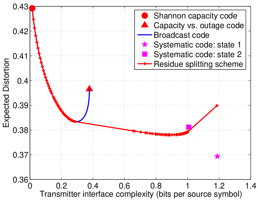
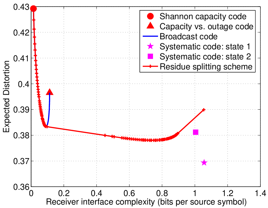
Expected distortion alone does not provide the complete picture for comparison of the schemes. In Fig. 9 and 10 we assume the channel state probability $p=0.7$ and illustrate the tradeoff between the expected distortion and the transmitter/receiver interface complexity for different schemes, where the complexity is measured by bits per source symbol delivered through the interface. For the broadcast scheme, we can reduce the expected distortion by increasing $\beta$ , which reduces the base layer rate but increases the refinement layer rate and the total rate, hence a higher interface complexity. However, the distortion-complexity curve is not strictly decreasing. After we reach the minimum expected distortion, it does not provide any more benefit to further increase the interface complexity. The same trend is also observed in the residue splitting scheme. At channel state probability $p=0.7$ , the systematic code targeting the good state has the lowest expected distortion, nevertheless it also has the highest interface complexity. The choice about the appropriate scheme and operating points (parameters) depends on the system designer’s view about this distortion-complexity tradeoff.

VI Conclusions

We consider transmission of a stationary ergodic source over non-ergodic composite channels with channel state information at the receiver (CSIR). To study the source-channel coding problem for the entire system, we include a broader class of transmission schemes as separation schemes by relaxing the constraint of Shannon separation, i.e. a single-number comparison between source coding rate and channel capacity, and introducing the concept of a source-channel interface which allows the source and channel to agree on multiple parameters.

We show that different end-to-end distortion metrics lead to different conclusions about separation optimality, even for the same source and channel models. Specifically, one such generalized scheme guarantees the separation optimality under the distortion versus outage metric. Separation schemes are in general suboptimal under the expected distortion metric. We study the performance enhancement when the source and channel coders exchange more information through a more sophisticated interface, and illustrate the tradeoff between interface complexity and end-to-end performance through the example of transmission of a binary symmetric source over a composite binary symmetric channel.

Appendix A MR Source Code and BC Channel Code Structure

In Fig. 4, the multi-resolution source code can be constructed as follows. Consider three independent auxiliary random variables $V_{1}$ $\sim$ Bernoulli $(\lambda)$ , $V_{2}$ $\sim$ Bernoulli $(1/2)$ , and $Q_{1}$ $\sim$ Bernoulli $(D_{1})$ , where

\lambda=\frac{D_{2}-D_{1}}{1-2D_{1}}

and $D_{1}$ , $D_{2}$ are given by (44). Also define

Q_{2}=V_{1}\oplus Q_{1},

which has a Bernoulli distribution with parameter $\lambda*D_{1}=D_{2}$ . These variables are related to the source symbol through the relationship

V=V_{2}\oplus Q_{2}=V_{2}\oplus V_{1}\oplus Q_{1}.

Random codebook generation: Generate $2^{nbR_{2}}$ sequences $V^{n}_{2}(w_{2})$ , $w_{2}\in\{1,\cdots,2^{nbR_{2}}\}$ , by uniform and independent sampling over the strong typical set $T^{n}_{\delta}(V_{2})$ . Similarly, generate $2^{nbR_{1}}$ sequences $V^{n}_{1}(w_{1})$ , $w_{1}\in\{1,\cdots,2^{nbR_{1}}\}$ , drawn uniformly and independently over $T^{n}_{\delta}(V_{1})$ .

Encoding: Given $V^{n}\in\mathcal{V}^{n}$ , the encoder searches over $(w_{1},w_{2})\in\{1,\cdots,2^{nbR_{1}}\}\times\{1,\cdots,2^{nbR_{2}}\}$ . If it finds a pair $(w_{1},w_{2})$ such that

(V^{n},V^{n}_{1}(w_{1}),V^{n}_{2}(w_{2}))\in T^{n}_{\delta}(V,V_{1},V_{2}),

it stops the search and sends the above $(w_{1},w_{2})$ . Otherwise it sends $(w_{1},w_{2})=(1,1)$ .

Decoding: If only the index $w_{2}$ is received, the decoder declares the estimate of the source sequence as $\hat{V}^{n}_{2}=V^{n}_{2}(w_{2})$ . If both indices are received, the source is reconstructed as $\hat{V}^{n}=\hat{V}^{n}_{1}\oplus\hat{V}^{n}_{2}=V^{n}_{1}(w_{1})\oplus V^{n}_{2}(w_{2})$ . Following the procedures in [38] and [39, Theorem 1] we can easily verify the following distortion targets are achievable: $\mathbb{E}d(V^{n},\hat{V}^{n})\leq D_{1}$ , $\mathbb{E}d(V^{n},\hat{V}^{n}_{2})\leq D_{2}$ .

In practice the MR source code can be implemented as a multi-stage vector quantization, which has an additive successive refinement structure [39]. As shown in Fig. 4, in channel state 2 only the base layer description is received and Source DEC 2 determines the base reconstruction $\hat{V}_{2}^{n}$ . When both layers are received, Source DEC 1 determines a refinement sequence $\hat{V}_{1}^{n}$ based on the refinement layer encoding index only, and add it to the base reconstruction $\hat{V}_{2}^{n}$ to obtain the overall reconstruction $\hat{V}^{n}$ . On the contrary, for general MR source codes the overall reconstruction may require a joint decoding of indices from both layers. The additive refinement structure reduces coding complexity, provides scalability, and does not incur any performance loss under certain conditions [39, Theorem 3], which are all satisfied in this example.

The broadcast channel code design, for a chosen $0\leq\beta\leq(1/2)$ , is summarized as follows.

Random codebook generation: Generate $2^{nbR_{2}}=2^{mR_{2}}$ independent codewords $U^{m}(w_{2})$ , $w_{2}\in\{1,\cdots,2^{mR_{2}}\}$ , by i.i.d. sampling of a Bernoulli $(1/2)$ distribution. Generate $2^{nbR_{1}}=2^{mR_{1}}$ independent codewords $Q_{\beta}^{m}(w_{1})$ , $w_{1}\in\{1,\cdots,2^{mR_{1}}\}$ , by i.i.d. sampling of a Bernoulli $(\beta)$ distribution.

Encoding: To send the index pair $(w_{1},w_{2})$ , send $X^{m}=Q_{\beta}^{m}(w_{1})\oplus U^{m}(w_{2})$ .

Decoding: Given channel output $Z^{m}$ , in state 2 we determine the unique $\hat{\hat{w}}_{2}$ such that

d(Z^{m},U^{m}(\hat{\hat{w}}_{2}))\leq(\alpha_{2}*\beta).

In state 1 we look for the unique indices $(\hat{w}_{1},\hat{w}_{2})$ such that

	$\displaystyle d(Z^{m},U^{m}(\hat{w}_{2}))\leq(\alpha_{1}*\beta),$
	$\displaystyle d(Z^{m},Q_{\beta}^{m}(\hat{w}_{1})\oplus U^{m}(\hat{w}_{2}))\leq\alpha_{1}.$

Following the analysis of [29, Theorem 14.6.2], we can show that the channel decoding error probability approaches zero as long as the encoding rates satisfy (43).

Roughly speaking, in channel state 2, we observe

Z^{m}=X^{m}\oplus Q_{\alpha_{2}}^{m}=U^{m}\oplus Q_{\beta}^{m}\oplus Q_{\alpha_{2}}^{m},

where the channel noise $Q_{\alpha_{2}}^{m}$ is a Bernoulli $(\alpha_{2})$ sequence. We want to decode the $U^{m}$ sequence subject to the overall interference-plus-noise $Q_{\beta}^{m}\oplus Q_{\alpha_{2}}^{m}$ , which is a Bernoulli sequence with parameter $(\alpha_{2}*\beta)$ , hence the achievable rate $1-h(\alpha_{2}*\beta)$ . In channel state 1, we observe

Z^{m}=X^{m}\oplus Q_{\alpha_{1}}^{m}=U^{m}\oplus Q_{\beta}^{m}\oplus Q_{\alpha_{1}}^{m}.

Since $\alpha_{1}<\alpha_{2}$ , the sequence $U^{m}$ can be decoded and then subtracted off. We then decode $Q_{\beta}^{m}$ subject to the noise $Q_{\alpha_{1}}^{m}$ , and the rate $h(\alpha_{1}*\beta)-h(\alpha_{1})$ is achievable.

References

[1] T. S. Han. Information-Spectrum Method in Information Theory. Applications of mathematics. Springer, New York, NY, 2003.
[2] R. Ahlswede. The weak capacity of averaged channels. Z. Wahrscheinlichkeitstheorie und Verw. Gebiete, 11:61–73, 1968.
[3] S. Verdú and T. S. Han. A general formula for channel capacity. IEEE Trans. Inform. Theory, 40(4):1147–1157, July 1994.
[4] M. Effros and A. Goldsmith. Capacity definitions and coding strategies for general channels with receiver side information. In Proc. IEEE Int. Symp. Inform. Theory (ISIT), page 39, Cambridge MA, August 1998.
[5] M. Effros, A. Goldsmith, and Y. Liang. Capacity definitions for general channels with receiver side information. Submitted to IEEE Trans. Inform. Theory, April 2008. Available at http://arxiv.org/abs/0804.4239.
[6] L. Ozarow, S. Shamai, and A. Wyner. Information theoretical considerations for cellular mobile radio. IEEE Trans. Veh. Tech., 43(2):359–378, May 1994.
[7] G. Foschini and M. Gans. On limits of wireless communications in a fading environment when using multiple antennas. Wireless Personal Comm., 6:311–335, March 1998.
[8] A. Goldsmith, S. A. Jafar, N. Jindal, and S. Vishwanath. Capacity limits of MIMO channels. IEEE J. Sel. Areas Commun., 21(5):684–702, June 2003.
[9] L. Zheng and D. N. C. Tse. Diversity and multiplexing: a fundamental tradeoff in multiple antenna channels. IEEE Trans. Inform. Theory, 49:1073–1096, May 2003.
[10] A. Goldsmith. Wireless Communications. Cambridge University Press, New York NY, 2005.
[11] S. Shamai and A. Steiner. A broadcast approach for a single-user slowly fading MIMO channel. IEEE Trans. Inform. Theory, 49(10):2617–2635, Oct. 2003.
[12] M. Effros, A. Goldsmith, and Y. Liang. Capacity definitions of general channels with receiver side information. In Proc. IEEE Int. Symp. Inform. Theory (ISIT), pages 921–925, Nice, France, June 2007.
[13] K. Zachariadis, M. Honig, and A. Katsaggelos. Source fidelity over a two-hop fading channel. In IEEE MilCom, pages 134–139, Monterey CA, Nov. 2004.
[14] D. Gündüz and E. Erkip. Joint source-channel codes for MIMO block-fading channels. IEEE Trans. Inform. Theory, 54(1):116–134, Jan. 2008.
[15] C. T.K. Ng, D. Gündüz, A. Goldsmith, and E. Erkip. Recursive power allocation in Gaussian layered broadcast coding with successive refinement. In IEEE Int. Conf. Communications, Glasgow, Scotland, June 2007. To appear.
[16] C. T.K. Ng, D. Gündüz, A. Goldsmith, and E. Erkip. Minimum expected distortion in Gaussian layered broadcast coding with successive refinement. In Proc. IEEE Int. Symp. Inform. Theory (ISIT), pages 2226–2230, Nice, France, June 2007.
[17] S. Shamai, S. Verdú, and R. Zamir. Systematic lossy source/channel coding. IEEE Trans. Inform. Theory, 44(2):564–579, March 1998.
[18] Z. Reznic, M. Feder, and R. Zamir. Distortion bounds for broadcasting with bandwidth expansion. IEEE Trans. Inform. Theory, 52(8):3778–3788, August 2006.
[19] U. Mittal and N. Phamdo. Hybrid digital-analog (HDA) joint source-channel codes for broadcasting and robust communications. IEEE Trans. Inform. Thoery, 48(5):1082–1102, May 2002.
[20] I. Csiszár and J. Körner. Information Theory: Coding Theorems for Discrete Memoryless Systems. Academic Press, New York, 1981.
[21] C. Shannon. A mathematical theory of communication. Bell Sys. Tech. Journal, 27:379–423, 623–656, July, Oct. 1948.
[22] R. L. Dobrushin. General formulation of Shannon’s main theorem in information theory. Amer. Math. Soc. Trans., 33:323–438, 1963.
[23] G. D. Hu. On Shannon theorem and its converse for sequence of communication schemes in the case of abstract random variables. In Proc. 3rd Prague Conf. on Inform. Theory, Stat. Decision Functions, Random Processes, pages 285–333, Czechoslovak Academy of Sciences, Prague, 1964.
[24] M. Gastpar, B. Rimoldi and M. Vetterli. To code, or not to code: lossy source-channel communication revisited. IEEE Trans. Inform. Theory, 49(5):1147–1158, May 2003.
[25] T. Berger. Rate Distortion Theory: a Mathematical Basis for Data Compression. Prentice-Hall, Englewood Cliffs, NJ, 1971.
[26] T. Cover, A. El Gamal, and M. Salehi. Muliple access channels with arbitrarily correlated sources. IEEE Trans. Inform. Theory, 26(6):648–657, Nov. 1980.
[27] S. Vembu, S. Verdú, and Y. Steinberg. The source-channel separation theorem revisited. IEEE Trans. Inform. Theory, 41(1):44–54, Jan. 1995.
[28] Y. Liang, A. Goldsmith, and M. Effros. Distortion metrics of composite channels with receiver side information. In IEEE Inform. Theory Workshop (ITW), pages 559–564, Lake Tahoe, CA, Sept. 2007.
[29] T. Cover and J. Thomas. Elements of Information Theory. Wiley & Sons, Inc., 1991.
[30] T. Cover. Broadcast channels. IEEE Trans. Inform. Theory, 18:2–14, Jan. 1972.
[31] R. Gallager. Information Theory and Reliable Communication. New York: Wiley, 1968.
[32] W. Equitz and T. Cover. Successive refinement of information. IEEE Trans. Inform. Theory, 37(2):269–275, March 1991.
[33] C. Tian, A. Steiner, S. Shamai(Shitz), and S. Diggavi. Expected distortion for Gaussian source with a broadcast transmission strategy over a fading channel. In Proc. IEEE Inform. Theory Workshop on Wireless Networks, pages 1–5, Bergen Norway, July 2007.
[34] M. Skoglund, N. Phamdo, and F. Alajaji. Design and performance of VQ-based hybrid digital-analog joint source-channel codes. IEEE Trans. Inform. Theory, 48(3):708–720, March 2002.
[35] A. Gersho and R. M. Gray. Vector quantization and signal compression. Kluwer, Boston MA, 1992.
[36] A. D. Wyner and J. Ziv. The rate-distortion function for source coding with side information at the decoder. IEEE Trans. Inform. Theory, 22(1):1–10, Jan. 1976.
[37] S. B. Wicker. Error control systems for digital communication and storage. Prentice Hall, Englewood Cliffs, NJ, 1995.
[38] A. El Gamal and T. M. Cover. Achievables rates for multiple descriptions. IEEE Trans. Inform. Theory, 28:851–857, Nov. 1982.
[39] E. Tuncel and K. Rose. Additive successive refinement. IEEE Trans. Inform. Theory, 49(8):1983–1991, August 2003.