Vacuum Stability of the $\mathcal{PT}$-Symmetric $\left(-\phi^{4}\right)$ Scalar Field Theory

Among its wide range of applications, the subject of $\mathcal{PT}$-symmetric theories has stressed the bounded-from-above $(-x^{4})$ quantum mechanical potential [1, 2, 3, 4, 5, 6]. The recipe for the calculations within such theories is to choose a specific contour in the complex $x$-plane and apply the quantization condition ($\chi_{n}\rightarrow 0$ as $\left|x\right|\rightarrow\infty$) on the wave functions $\chi_{n}$. It is this boundary condition that renders the problem non-Hermitian and $\mathcal{PT}$-symmetric as well. For the complete determination of the transition amplitudes within the $\mathcal{PT}$-symmetric theories, the positive definite metric operator and thus the equivalent Hermitian Hamiltonian have to be obtained. This has been done for the $\mathcal{PT}$-symmetric ($-x^{4}$) theory in Ref. [5]. Remarkably, the equivalent Hermitian Hamiltonian is bounded from below. This gives no doubt that the spectrum of the $\mathcal{PT}$-symmetric ($-x^{4}$) theory is stable. However, in higher space-time dimensions i.e. for quantum field problems, the treatment of the theory on a complex contour is hard to follow, because it is possible to have complicated Jacobian factors [7].

To avoid the existence of complicated Jacobian factors within the study of a $\mathcal{PT}$-symmetric theory on a complex contour, one may seek a way to modify the recipe used in quantum mechanical $\mathcal{PT}$-symmetric problems in a manner that makes it applicable for $\mathcal{PT}$-symmetric field theories. The usual recipe to study $\mathcal{PT}$-symmetric quantum theories mentioned above has shown that the spectrum of the $\mathcal{PT}$-symmetric $\left(-x^{4}\right)$ is bounded from below, although the classical potential $\left(-x^{4}\right)$ is unstable. Therefore, the mentioned algorithm can advocate the vacuum stability for the theory in $0+1$ space-time dimensions. Before we go on, we need to assert that for $\mathcal{PT}$-symmetric quantum field theories, there exists a lack of studies in the literature that discuss the vacuum stability for unstable classical potentials like that of the $\mathcal{PT}$-symmetric $\left(-\phi^{4}\right)$ field theory. In this work, we apply an algorithm which mimics the usual complex contour method, and it avoids the problems associated with its direct extension to quantum field problems. As we will show in this work, the algorithm we use can explain the stability of the vacuum of the the $\mathcal{PT}$-symmetric $\left(-\phi^{4}\right)$ field theory for which classical analysis prohibits vacuum stability. In fact, the algorithm can be applied to any quantum field theory but we use the $\mathcal{PT}$-symmetric $\left(-\phi^{4}\right)$ theory as an illustrative example.

The algorithm we follow to study a $\mathcal{PT}$-symmetric field theory is in the same spirit as the known complex contour method applied to the quantum mechanical cases [1, 2, 3, 4, 5]. In this algorithm, we follow the canonical quantization method in which the Hamiltonian determines the dynamics of the system [9]. Therefore, the non-Hermiticity of the theory can be realized. Moreover, the canonical quantization method employs two important features; (i) the equal time canonical commutation relations and (ii) the Heisenberg picture for the operators which leads the field to verify the Heisenberg equation of motion. These features let the amplitudes obtained through this algorithm to know about the metric [10, 11]. Accordingly, the algorithm we use avoids the calculation of the metric operator, which is hard to get for the $\mathcal{PT}$-symmetric $\left(-\phi^{4}\right)$ field theory [11].

To account for the complex contour in the method we apply, we shift the field $\phi$ to $\psi+B$, where $B$ is a $C$-number representing the vacuum condensate. The field $\psi$ is real and has a different mass, while the condensate is to be determined from the effective potential by constraining it to satisfy the following stability conditions;

where $M$ is the renormalized mass of the field $\psi$. Since the renormalized mass is always chosen to be real and positive, the effective potential as a function of the condensate $B$ is bounded from below. However, as we will see later, in this case $B$ ought to be imaginary, and thus the contour $\psi+B$ is complex. Hence, the resulting effective theory is non-Hermitian but $\mathcal{PT}$-symmetric, which secures the reality of spectrum.

The conditions in Eq.(I.1) guarantee a bounded-from-below effective potential, and also agree with the known constraints applied to the effective potential [9, 12]. In fact, the condition $\frac{\partial V_{eff}}{\partial B}=0$ is used to kill tad pole diagrams [9], while $\frac{\partial^{2}V_{eff}}{\partial B^{2}}=M^{2}$ represents the mass renormalization condition [12]. To give an idea about how this algorithm mimics the famous complex contour method, we mention that in quantum mechanical studies we used to have localized wave functions ($\chi\rightarrow 0$ as $x\rightarrow\infty$) associated with bounded-from-below potentials. Apparently, the conditions $\frac{\partial V_{eff}}{\partial B}=0$ and $\frac{\partial^{2}V_{eff}}{\partial B^{2}}=M^{2}$ define a minimum in the effective potential. Therefore, the algorithm mimics the quantization condition $\chi\rightarrow 0$ as $\left|x\right|\rightarrow\infty$, applied in the complex contour method. Within this regime, the field shift $\phi\rightarrow\psi+B$ with $B$ imaginary resembles the choice of a complex contour. For some theories, the spectrum is sensitive to the boundary condition $\chi\rightarrow 0$ as $\left|x\right|\rightarrow\infty$, and thus the theory has different spectra for different contours. In this case, in our algorithm, the conditions;

lead to different $B$ solutions, and the theory will have different vacua defined by different condensate solutions.

For a quantitative test for the algorithm mentioned above in the study of $\mathcal{PT}$-symmetric problems, we refer to our previous work in Ref.[6]. There, we applied the effective field algorithm for the calculations within the quantum mechanical $\mathcal{PT}$-symmetric $\left(-x^{4}\right)$ theory. We found reasonable results for the energy spectrum and the vacuum condensate compared to exact results. Also, we obtained the relations;

for the vacuum condensate $B$ and the effective mass of the massless $\mathcal{PT}$-symmetric $\left(-x^{4}\right)$ theory. These relations have been reproduced by Jones in Ref. [11] using the Schwinger-Dyson equations ¹¹ 1 Take into account the relations between our coupling and their coupling $\left(\lambda=2g\right)$ and a rescaling $\frac{1}{2}$ to their Hamiltonian is to be taken into account. Such kind of interesting results support the extension of the algorithm to quantum field theories (higher dimensions) which is our aim in this work. In fact, we will tackle the point of vacuum stability of the $\mathcal{PT}$-symmetric $\left(-\phi^{4}\right)$ theory, which has not been stressed before in the literature. However, since in higher dimensions there exist UV divergences in the calculations, one has to employ known tools to cure them. For that, the algorithm we apply starts by using a normal ordered theory. To eliminate divergences at the first order in the coupling, one normal order the theory with respect to another mass parameter. This technique has been used in the context of super renormalizable quantum field theories in Refs.[13, 14].

The paper is organized as follows. In Section II, the formulation of the effective field method is introduced. The calculation of the effective potential up to $g^{1}$ and $g^{2}$ order of approximations for the $\mathcal{PT}$-symmetric $\left(-\phi^{4}\right)$ field theory in $1+1$ space-time dimensions is presented in Section III, while the $2+1$ case is considered in Section IV. In Section V, the discussions and conclusions are introduced.

In the absence of an external source, the effective potential is equivalent to the vacuum energy $E$ ( $E=\langle 0|H|0\rangle$). To illustrate the implementation of the above mentioned ideas for the calculation of the effective potential of the $\mathcal{PT}$-symmetric $\left(-\phi^{4}\right)$ theory, we start by the Hamiltonian density of the form;

in which $N_{m}$ indicates that $H$ is a normal-ordered form with respect to the vacuum of the field $\phi$ of mass $m$. In introducing the field shift $\phi\rightarrow\psi+B$ , the Hamiltonian density takes the form;

Also, in taking into account the relation [13];

one can obtain the resulting Hamiltonian normal-ordered with respect to the new mass parameter $M$ of the effective field $\psi$. To show this, we first note that this relation can lead to the following set of relations;

where $\Delta$ is the free field two point function [13]. For the kinetic term, we can get the result;

where

Here $D$ is the dimension of the space-time. Considering these forms, one can rewrite the Hamiltonian density $H$ in Eq.(II.1) in the form;

In fact, $\Delta$ and $E_{0}$ might be divergent in space-time dimensions higher than one. The divergences can be eliminated as it was done by Coleman in Ref. [13], where the propagator of mass $m$ is subtracted from that of the mass $M$ of the effective field. In Ref. [15], this regularization method has been used also to regularize the sunset diagram. So, we shall use this regularization method even for contributions to the effective potential beyond the normal ordering result.

The effective potential, or equivalently the vacuum energy can be obtained from Eq.(II) where normal-ordered fields result in zero vacuum expectation values, and thus do not contribute to the effective potential. In the formula above for the effective Hamiltonian, the quantities $\Delta$ and $E_{o}$ depend on the dimension of the space-time. Accordingly, we will study the $1+1$ and $2+1$ cases individually.

The Hamiltonian form in Eq.(II) includes the space-time dependent terms $\Delta$ and $E_{o}$. In $1+1$ space-time dimensions, one can expand $E_{o}(\Omega)$ in Eq.(II.5) as a power series in $\epsilon=D-2$ to get the result;

and thus, we obtain the following form;

This is exactly the result obtained in Ref.[13]. The vacuum energy is then given by;

with $\Delta=-\frac{1}{4\pi}\ln t$ and $t=\frac{M^{2}}{m^{2}}$. This result has been obtained relying on the fact that the vacuum expectation values of the normal-ordered operators in Eq. (II) are certainly zero, and we are left with the field-independent terms (last line in Eq.(II)). To cure the divergences that appear in the calculations of $\Delta$, we subtracted the propagator with mass $m$ from that with $M$ as in Ref. [13].

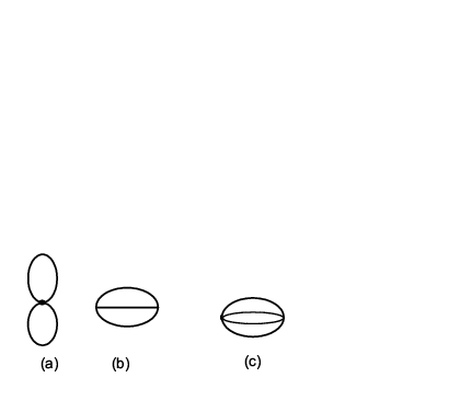
The above result for the vacuum energy accounts for the contribution of the one vertex Feynman diagram ( diagram (a) in Fig.1) to the effective potential. In the absence of external source, the effective potential is equivalent to the vacuum energy [9], and it has to satisfy the conditions [12];

In using the parameters redefinition; $b^{2}=4\pi B^{2}$, $t=\frac{M^{2}}{m^{2}}$, and $G=\frac{g}{2\pi m^{2}}$, one gets;

The condition $\frac{\partial E}{\partial B}=0$ leads to the relation

where for $b\neq 0$, it results in the solution $t=\exp\left(\frac{1}{3}\frac{Gb^{2}-2}{G}\right)$. In using the relation; $\frac{\partial^{2}E\left(M,B,g\right)}{\partial B^{2}}=M^{2}$, one can show that $b^{2}=\frac{-t}{G}$, but in this case both conditions in Eq.(III.4) are used which means that the obtained parameters ($b$ and $t$) define the minimum of the effective potential. Equivalently, we get the result;

where $W$ is the Lambert’s $W$ function defined by $W(x)e^{W(x)}=x$. Note that $W\left(x\right)=\allowbreak x+O\left(x^{2}\right)$, for small values of the argument $x$. Therefore, we obtain the result;

This exponential behavior for the dependence of the vacuum condensate on the coupling has been obtained before in Ref. [8], which constitutes a good test for our calculations.

To advocate the vacuum stability, one can use the the relation $t=\exp\left(\frac{1}{3}\frac{Gb^{2}-2}{G}\right)$ to plot the vacuum energy in Eq.(III.5). As shown in Fig. 2, the effective potential is bounded from below, and thus the plot shows the stability of the vacuum state. This result is pretty interesting, as it is the first time to show that the vacuum of the $\mathcal{PT}$-symmetric $\left(-\phi^{4}\right)$ scalar field theory is stable in $1+1$ space-time dimensions.

A note to be mentioned is that for imaginary $b$, the effective Hamiltonian obtained in Eq.(II) is non-Hermitian, but it is $\mathcal{PT}$-symmetric. Also, the $B\psi^{3}$ term turns the theory well defined on the real line [3].

One can go beyond the above result for the vacuum energy and include the radiative corrections received from the sunset ( diagram (b) in Fig.1), and the watermelon ( diagram (c) in Fig.1) diagrams. These diagrams constitute the $G^{2}$ contribution to the effective potential, which then takes the form;

with $\beta=3.155$ and $\alpha=\frac{1}{2}\left(\Psi\left(\frac{1}{3},1\right)-\Psi\left(\frac{2}{3},1\right)\right),$ while $\Psi\left(x,n\right)=\frac{d^{n+1}}{dx^{n+1}}\ln\Gamma\left(x\right)$ ( see the appendix for the calculation of the Feynman diagrams).

In applying the condition $\frac{\partial E}{\partial B}=0,$ the coefficient of $\psi$ is always zero, and thus the above result does not include Feynman diagrams resulting from the $\psi$ term in the Hamiltonian in Eq.(II). Accordingly, the stability requirement for which one always subject $E$ to the condition $\frac{\partial E}{\partial b}=0$ then yields the result;

For $b\neq 0$, one can solve for $t$ to have the form;

where $x=\frac{2-Gb^{2}}{3G}$. Again, when we substitute this result in $E$ , and for $b$ imaginary, we get the bounded-from-below effective potential plotted in Fig. 3.

For further confirmation of the stability of the vacuum of the $\mathcal{PT}$-symmetric $\left(-\phi^{4}\right)$ scalar field theory in other space-time dimensions, we consider the $2+1$ dimensions case.

In this case, $\Delta$ in Eq.(II ) takes the form;

and $E_{0}(\Omega)$ in Eq.(II.5) is given by;

After substituting for the values of $\Delta$ and $E_{0}$ in Eq.(II), we get;

or,

where $G=\frac{g}{4\pi m}$, $t=\frac{M}{m}$, and $b=B\sqrt{\frac{4\pi}{m}}$. Since the most important corrections to the effective potential come from logarithmic contributions, one has to include at least the $G^{2}$ corrections to obtain a reliable contribution to the effective potential. This leads to the result;

Similar to the $1+1$ case, in applying the condition $\frac{\partial E}{\partial b}=0$, we get;

and for $b\neq 0$, we have

Again, in substituting this result into the form of $E$, we obtain the bounded- from-below effective potential shown in Fig.4. This is correct as long as $b$ is kept imaginary. Also, one can follow the same argument led to Eq.(III.8) for the $1+1$ case to show that the $b$ value at the minimum of the effective potential behaves like;

Such exponential behavior has also been obtained in Ref.[8], which constitutes a good check for the accuracy of our calculations.

We employed the canonical quantization method for the calculation of the effective potential for the $\mathcal{PT}$-symmetric $\left(-\phi^{4}\right)$ scalar field theory. We considered the cases of the $1+1$ and $2+1$ space-time dimensions individually. We have done that although in the literature the effective potential is often studied within the path integral formulation of the theory [9]. In fact, the path integral formulation by itself is obtained via the canonical quantization of the theory, for which the equal time canonical relations of the form;

are satisfied. Our point in following the canonical quantization method is that, with in this regime, the Hamiltonian operator determines the dynamics of the system. Therefore, the non-Hermiticity of the Hamiltonian operator for a $\mathcal{PT}$-symmetric field theory can be realized easily. So, we find it more plausible to work with operators ( canonical quantization) than working with integration over classical functionals ( path integral). Note that, in the canonical quantization of a theory, one also employs the Heisenberg picture for the operators ( see the chapters in the first part in Ref.[9]). Thus, for the theory under consideration, the Heisenberg equation of motion is satisfied. Accordingly, the calculated amplitudes know about the metric [10, 11]. This means that the followed algorithm in our work avoids the calculation of the metric operator, which is hard to get for the theory under consideration.

For the $\mathcal{PT}$-symmetric $\left(-\phi^{4}\right)$ scalar field theory, the classical potential is bounded from above. Consequently, the common classical analysis predicts an unstable vacuum. In our work, we have shown that the effective potential is bounded-from-below which shows that the vacuum state of the $\mathcal{PT}$-symmetric $\left(-\phi^{4}\right)$ scalar field theory is stable. This result tells us that classical analysis are not always reliable either quantitatively or qualitatively.

The stability of the theory is constrained by the existence of an imaginary condensate. The imaginary value of the condensate renders the effective theory non-Hermitian but $\mathcal{PT}$-symmetric. In fact, the effective theory is well defined on the real line because of the existence of the pure imaginary, $B\psi^{3}$, term in the Hamiltonian.

To test the accuracy of our results, we obtained the vacuum condensate at the minimum of the effective potential. The behavior of the condensate has been found to approach its zero value for small coupling in an exponential manner ( Eq.(III.8)&Eq.(IV.8)). This exponential behavior has been obtained before in Ref.[8], which represents a good test for the accuracy of our results.

This work sheds light on some how a new strange behavior of the quantum world. It tells us that classical analysis does not always rule the quantum behavior of a quantum particle. The situation is very similar to the tunneling effect in quantum physics for which classical analysis totally prohibits tunneling from existence, while the quantum world admits it. Likewise, the vacuum stability is totally prohibited from a classical point of view for bounded- from-above potentials, while we have shown that the potential felt by the quantum particle is bounded from below, and thus allows a stable vacuum.

Appendix: Feynman Diagram Calculations

References

• [1] Carl Bender and Stefan Boettcher, Phys.Rev.Lett.80:5243-5246 (1998).
• [2] H. F. Jones and R. J. Rivers, Phys.Rev.D75:025023 (2007).
• [3] Carl M. Bender, Dorje C. Brody and Hugh F. Jones, Phys.Rev.D73:025002(2006).
• [4] H. F.Jones, J. Mateo and R. J. Rivers Phys.Rev.D74:125022 (2006).
• [5] H. F. Jones, J. Mateo, Phys.Rev.D73:085002 (2006).
• [6] Abouzeid M.Shalaby, Phys. Rev. D 79, 065017 (2009).
• [7] Carl M. Bender, Dorje C. Brody, Jun-Hua Chen, Hugh F. Jones, Kimball A. Milton, and Michael C. Ogilvie1, Phys.Rev. D 74, 025016 (2006).
• [8] Carl M. Bender, Peter N. Meisinger, and Haitang Yang, Phys.Rev. D63, 045001 (2001).
• [9] Book by Michael E.Peskin and Daniel V.Schroeder, ”AN INTRODUCTION TO THE QUANTUM FIELD THEORY” (1995).
• [10] H. F. Jones and R. J. Rivers, Phys. Lett. A 373, 3304 (2009).
• [11] H.F. Jones, Int J Theor Phys 50: 1071–1080 (2011) .
• [12] LEWIS H. RYDER , Quantum Field Theory (Second edition , CAMBRIDGE UNIVERSITY PRESS ) ( 1996).
• [13] Sideny Coleman, Phys.Rev.D11:2088 (1975).
• [14] S. J. Chang, Phys. Rev. D 13, 2778 (1976) [Erratum-ibid. D 16, 1979 (1976)].
• [15] Steven F. Magruder, Phys. Rev. D 14, 1602 (1976).
• [16] Jing-Ling Chen, L.C. Kwek and C.H.Oh, Phys. Rev. A 67, 012101 (2003).
• [17] Carl M. Bender , Dorje C. Brody and Hugh F. Jones, Phys.Rev.D73:025002 (2006 ).
• [18] John C. Collins, RENORMALIZATION, CAMBRIDGE UNIVERSITY PRESS (1984).
• [19] Arttu K. Rajantie, Nucl.Phys. B480 ,729-752 ((1996)); Erratum-ibid. B513, 761-762 (1998).
Refer to caption
.
Figure 2: The effective potential e=8​π​Em2e=\frac{8\pi E}{m^{2}}, up to order G1G^{1}, versus the vacuum condensate bb for G=12G=\frac{1}{2} for the 𝒫​𝒯\mathcal{PT}-symmetric(−ϕ4)\left(-\phi^{4}\right) scalar field theory in 1+11+1 space-time dimensions.
Figure 3: The effective potential e=8​π​Em2e=\frac{8\pi E}{m^{2}} versus the vacuum condensate bb for G=12G=\frac{1}{2} for the 𝒫​𝒯\mathcal{PT}-symmetric(−ϕ4)\left(-\phi^{4}\right) scalar field theory in 1+11+1 space-time dimensions, and up to G2G^{2} order in the coupling.
Figure 4: The effective potential e=8​π​Em3e=\frac{8\pi E}{m^{3}}, up to order G2G^{2}, versus the vacuum condensate bb for G=12G=\frac{1}{2} for the 𝒫​𝒯\mathcal{PT}-symmetric(−ϕ4)\left(-\phi^{4}\right) scalar field theory in 2+12+1 space-time dimensions.