Elastic capsules in shear flow:
Analytical solutions for constant and time-dependent shear rates
Abstract
We investigate the dynamics of microcapsules in linear shear flow within a reduced model with two degrees of freedom. In previous work for steady shear flow, the dynamic phases of this model, i.e. swinging, tumbling and intermittent behaviour, have been identified using numerical methods. In this paper, we integrate the equations of motion in the quasi-spherical limit analytically for time-constant and time-dependent shear flow using matched asymptotic expansions. Using this method, we find analytical expressions for the mean tumbling rate in general time-dependent shear flow. The capsule dynamics is studied in more detail when the inverse shear rate is harmonically modulated around a constant mean value for which a dynamic phase diagram is constructed. By a judicious choice of both modulation frequency and phase, tumbling motion can be induced even if the mean shear rate corresponds to the swinging regime. We derive expressions for the amplitude and width of the resonance peaks as a function of the modulation frequency.
pacs
87.16.D-Membranes, bilayers, and vesicles and 47.15.G-Low-Reynolds-number (creeping) flows1 Introduction
The dynamic motion of soft objects such as elastic microcapsules in shear flow represents a long-standing problem in science and engineering. It has received increasing interest recently, in particular due to its relevance to biological, medicinal and microfluidic applications. This problem is challenging from a theoretical point of view, because the shape of these objects is not given a priori, but determined dynamically from a balance of interfacial forces with fluid stresses. New insight has been gained due to a plethora of experimental Eggleton and Popel (1998); Walter et al. (2001); Fischer (2004); Abkarian et al. (2007); Fischer (2007), theoretical Barthès-Biesel (1980); Barthès-Biesel and Rallison (1981); Keller and Skalak (1982); Barthes-Biesel and Sgaier (1985); Barthès-Biesel et al. (2002); Lac et al. (2004); Lac and Barthès-Biesel (2005); Finken and Seifert (2006); Skotheim and Secomb (2007), and numerical Pozrikidis (1995); Ramanujan and Pozrikidis (1998); Noguchi and Gompper (2005); Kessler et al. (2007); Sui et al. (2008a); Sui et al. (2008b); Dodson III and Dimitrakopoulos (2008) methods.
Perhaps the most well-known dynamic state of initially spherical elastic microcapsules in shear flow is the tank-treading motion also present in fluid vesicles Kraus et al. (1996); de Haas et al. (1997); Seifert (1999); Pozrikidis (2001); Noguchi and Gompper (2004); Kantsler and Steinberg (2005); Kantsler and Steinberg (2006); Misbah (2006); Vlahovska and Gracia (2007); Lebedev et al. (2007), as reviewed in the first two chapters of Pozrikidis (2003). In contrast to fluid vesicles, microcapsules exhibit a finite shear elasticity, since their membrane is chemically or physically cross-linked. This holds both for artificial polymerised capsules Walter et al. (2001) and red blood cells (RBCs), whose membrane is composed of an incompressible lipid bilayer underlined by a thin elastic cytoskeleton Mohandas and Evans (1994). For a short time, viscous fluid vesicles can also resist shear.
The resistance to shear leads to qualitatively different behaviour, such as preventing the prolate to oblate shape transition of viscous fluid vesicles Noguchi and Gompper (2005). Perhaps most surprisingly, it also leads to qualitatively different instabilities like wrinkling first observed on polymerised capsules Walter et al. (2001); Finken and Seifert (2006) and later as a transient on viscous vesicles Kantsler et al. (2007).
When the unstressed initial shape of the cell is not spherical, material elements of the membrane are deformed when displaced from their initial position. This shape memory, suggested for RBCs in Ref. Fischer (2004), leads to an oscillation of the inclination angle superimposed on the tank-treading motion, called swinging, and an intermittent regime between tank-treading and tumbling Abkarian et al. (2007); Skotheim and Secomb (2007). The swinging motion of RBCs was studied numerically in Ref. Ramanujan and Pozrikidis (1998) using a boundary integral formulation of the hydrodynamics. Later, more comprehensive studies of all dynamic phases were performed using both a spectral numerical method Kessler et al. (2007) and an immersed boundary lattice Boltzmann method Sui et al. (2008a); Sui et al. (2008b). The phase diagram constructed in Ref. Kessler et al. (2007) basically confirmed the qualitative correctness of a reduced model Skotheim and Secomb (2007) at low to moderate viscosity ratios. However, both Refs. Kessler et al. (2007) and Sui et al. (2008b) independently contested the intermittent regime at large viscosity ratios as an artifact of the reduced model. Instead, in these works the tumbling motion was found to be a transient towards a stable swinging motion. Numerical studies of elongated capsules in extensional flow at high flow rates reveal a novel bifurcation between a spindled and a cusped capsule shape induced by compressive stresses Dodson III and Dimitrakopoulos (2008).
New phenomena are expected when the driving shear flow is no longer constant in time and space. Indeed, a transient wrinkling phenomenon was observed for fluid vesicles in suddenly reversed elongational shear flow Kantsler et al. (2007), where the stress becomes momentarily compressive. For spatially varying shear flow produced by structured microchannels, a transition from prolate shape to bullet-like shape as well as symmetry breaking transitions were observed in vesicles both experimentally and in simulations Noguchi et al. (2008).
So far, microcapsule dynamics has only been studied in steady shear flow. It is the aim of this paper to investigate the effects of modulating the shear rate on the dynamics of capsules. In particular, we want to focus on the question whether dynamic phase transitions can be induced by small amplitude oscillations around a fixed mean shear rate. Since solving the exact equations of motion numerically is computationally prohibitive, we constrain our investigations to the reduced model of Skotheim et al. Skotheim and Secomb (2007), which will allow analytical solutions in the quasi-spherical limit.
This paper is structured as follows: After reviewing the reduced model Skotheim and Secomb (2007), we derive non-dimensional equations of motion valid in the quasi-spherical limit in section 2. A numerical study of the dynamics for constant shear rate yields the dynamic phase diagram. In the quasi-spherical limit the equations of motion can be integrated exactly for time-constant shear flow, which is done in section 3. Integration is even possible for general time-dependent shear flow, which is studied in section 4 in detail. Specialising to harmonic modulations of the shear rate around a constant mean value reveals that tumbling motion can be induced from the swinging regime at certain resonance frequencies of the modulation. Both the resonance behaviour and the smooth off-resonance background are studied in detail. A dynamic phase diagram as a function of modulation amplitude and frequency is constructed. The more intricate details of the calculations are shown in the Appendices.
2 Reduced model

2.1 Equation of motion
We investigate a reduced model of an elastic capsule with fixed ellipsoidal shape (semi-axes , , , and volume ) in a linear shear flow with velocity
| (1) |
depending upon position and shear rate . The two axes and lie in the shear plane with (see Fig. 1). Thus the axis is perpendicular to the shear plane. The long axis is oriented with inclination angle with respect to the direction of the shear flow. The inner and outer flow have viscosities and , respectively. The membrane can tank-tread with respect to the fixed ellipsoidal shape, measured by the phase angle . This is the Keller-Skalak model for a Red Blood Cell Keller and Skalak (1982). Abkarian et al. Abkarian et al. (2007) and Skotheim and Secomb Skotheim and Secomb (2007) add an elastic energy term () which is due to the tank-treading motion and the shape memory effect Fischer (2004). Abkarian et al. Abkarian et al. (2007) also consider a viscosity of the membrane which effectively changes the inner viscosity. A Keller-Skalak-type Keller and Skalak (1982) derivation, which consists of a balance of torque and energy, yields the equations of motion for the angles and Skotheim and Secomb (2007):
| (2) | |||||
| (3) |
As the underlying equations of motion are overdamped, these equations hold also for time-dependent shear rate . The geometrical quantities depend only upon the semi-axes as given explicitly in Appendix A.
In the equations of motion (2) and (3) there are seven independent parameters, namely the hydrodynamic parameters , , , an elastic parameter and the geometric parameters , , which determine , , , . Three of them can be used to introduce independent scales. The volume defines a length scale, the shear rate of the external flow a time scale, and the elastic energy an energy scale.
a)

b)

Four independent parameters remain, i.e. the viscosity contrast , the ratio between hydrodynamic and elastic energy , the ratio of the short to the long axis in the shear plane , and the ratio of the axis perpendicular to the shear plane to the long axis . The first three can be used to define three equivalent nondimensional parameters, the shifted nondimensional viscosity contrast
| (4) |
(note that , , and for physical values), the capillary number
| (5) |
and the eccentricity parameter
| (6) |
Here, corresponds to the spherical case (), and corresponds to the case . It is convenient to introduce a dimensionless time by
| (7) |
which can also be done in the case of a positive time-dependent shear rate . We finally arrive at the nondimensional reformulation of the equations of motion
| (8) | |||||
| (9) |
where can be time-dependent. The phase space is the torus (each angle with period , see Fig. 2). Note that the fourth parameter does not enter the nondimensional equations of motion explicitly.
2.2 Mean tumbling rate and phase diagram
a)

b)

c)

d)

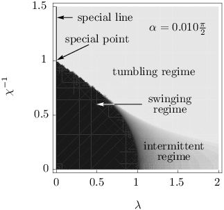
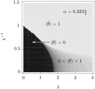
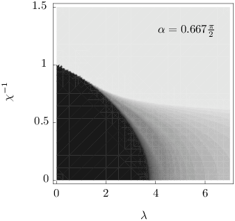
The solutions of the equations (8) and (9) in the case of a time-constant shear flow have been examined in Ref. Skotheim and Secomb (2007). The phase diagram consists of three different regimes depending upon the value of three parameters , , and . As shown in Fig. 3, the capsule can either tumble with a monotonously changing inclination angle and an oscillating phase angle or tank-tread with an oscillating inclination angle and a monotonously changing phase angle , a motion called swinging. There is a third regime in between, where the capsule both tumbles and tank-treads (either successivly or simultanously), which is called “intermittent” regime in Ref. Skotheim and Secomb (2007) (see Fig. 4). For low shear rates, i.e. for large values of , the hydrodynamic flow is too weak to overcome the elastic barrier due to the shape memory. Thus, the capsule tumbles for large . For smaller values of , i.e. for higher shear rates, the transition to the intermittent or swinging regime occurs.
a)
b)
c)
The dynamics in the reduced model can conveniently be characterized by investigating the normalized mean tumbling rate
| (10) |
as an order parameter. Here the mean rates of inclination and phase angle are given by
| (11) | |||||
| (12) |
respectively. In a stable tumbling motion, the inclination angle grows without bounds while the phase angle oscillates, which implies and a mean tumbling rate in the long time limit. Conversely, in a stable swinging motion, the phase angle grows without bounds while the inclination angle oscillates, which implies in the long time limit thus . In the intermittent regime, the mean tumbling rate takes values between and . Typical phase diagrams showing grey scale plots of the mean tumbling rate as obtained from solving equations (8) and (9) numerically can be seen in Fig. 4. Here, the axes consist of the dimensionless viscosity ratio and the inverse capillary number , while the eccentricity is constant.
Even though it is not central for this paper, we note for completeness that the status of the intermittent regime is still under debatte. Kessler et al. Kessler et al. (2007) and Sui et al. Sui et al. (2008b) solved the full dynamics of a 3d elastic capsule using a spectral method and a immersed boundary lattice Boltzmann method, respectively. While the reduced model captures the swinging and tumbling regime semi-quantitatively compared to fully numerical studies Kessler et al. (2007), the intermittent regime has been contested as an artifact of the reduced model. Neither study found any indications of intermittency, but rather a transition towards swinging. There was also no direct evidence of intermittent motion in experiments Abkarian et al. (2007).
2.3 Quasi-spherical case
Since the phase diagram is qualitatively similiar for all small values of (see Fig. 4), it is sufficient to investigate the quasi-spherical case, for which analytical progress becomes possible. We set where is a small parameter and assume the difference of to be also of order . The three dimensionless parameters introduced above then depend on to first order as (see Appendix B for definition of symbols)
| (13) | |||||
| (14) | |||||
| (15) |
In the quasi-spherical case, the elastic energy can be calculated for any elastic model. In the regime of small deformations the elastic energy scales quadratic with the eccentricity
| (16) |
with , leading to
| (17) |
For given values of all physical parameters, leaving aside the shear rate and the small parameter , the pre-factors in the above expansions (13), (14), and (17) are of the order of unity in the quasi-spherical limit . In this case, we are restricted to a small left hand stripe in the phase diagram (see Fig. 4) defined by . Here, the disputed intermittent regime has no influence on the dynamics and can be ignored. Since the transition between tumbling and swinging takes place at , we will later specify the shear rate to be of the order of the expansion parameter . For the following expansion we merely require the scaling of not to be smaller than .
Before we expand the equations of motion (8) and (9) in , we introduce a suitable stretched, rotated, and translated frame in the -plane (see Fig. 2) with coordinates
| (18) | |||||
| (19) |
where is, up to a constant, the angle of a tracer particle with respect to the direction of the shear flow. In these coordinates, the mean tumbling rate (10) can be written as
| (20) |
Finally, expansion of the equations of motion (8) and (9) up to first order in (note that , ) yields the quasi-spherical equations of motion in the new coordinates
| (21) | |||||
| (22) |
With the initial condition the solution of the first equation is
| (23) |
i.e. a tracer particle moves with constant angular velocity with respect to the dimensionless time . Assuming that the shear rate does not change sign, we can use the angle as a time quantity to arrive at an autonomous differential equation on the torus
| (24) |
where is now considered to be a function of rather than . Here, and are not restriced to the interval but can take all real values, thereby accounting for the number of revolutions on the torus.
3 Constant shear rate
We first summarize the big picture derived below in detail for the shape dynamics expressed by and close to the special line (see Fig. 4), corresponding to the quasi-spherical limit at fixed inverse capillary number . For a systematic expansion in , we first investigate the dynamics at the special line. We find a set of fixed points connected by curves, of which some are stable, some unstable, and some neutral (see Fig. 5). For capillary numbers , closed and separated curves in the phase space exist which consist solely of either stable or unstable fixed points. Upon perturbation to first order in these lines turn to stable or unstable limit cycles, as the perturbation does not alter the absolute stability. These limit cycles correspond to swinging and tumbling for and , respectively. At the special point , the lines of fixed points cross. Here, all vertical lines of fixed points consist solely of neutral fixed points, whereas all horizontal lines of fixed points consist of segments of either stable or unstable fixed points. Upon perturbation, the neutral fixed points can become either stable or unstable. Therefore the dynamics of the system close to the special point needs to be studied more carefully to first order in . Analytic determination of the resulting limit cycles becomes possible by considering the trajectories close to the stable, unstable, and neutral fixed points separately and joining these with the method of matched asymptotic expansion.
3.1 Zero order expansion on special line
We start by investigating the special line , where the equations of motion
| (25) | |||||
| (26) |
immediately lead to time-constant . For all values of there are two connected lines of fixed points (see Fig. 5) which bifurcate into limit cycles upon a perturbation with . The position and stability character of these lines of fixed points depend on the inverse capillary number . The corresponding regimes on the special line are seperated by the special point (, ).
At this special point, there are two straight lines of connected fixed points, namely with arbitrary and with arbitrary and integer . These lines of fixed points build up a checkerboard pattern as can be seen in Figs. 5 c) and 6.
a)

b)

c)

We now discuss the stability of each fixed point. The eigenvalue of a linearization around a fixed point in the direction of the connected fixed points is always zero. The sign of the other eigenvalue determines the stability of the fixed point in the perpendicular direction. Fixed points with a positive, negative or zero eigenvalue are called unstable, stable or neutral, respectively. The vertical lines of fixed points are neutral as is constant (25), while stable and unstable segments alternate on the horizontal lines as can be seen in Fig. 5 c), where the vector field corresponding to the equations of motion is shown. Thus, each square consists of two opposite neutral sides and two opposite lines of which one is stable and one is unstable.
3.2 First order expansion away from the transition
Since the system moves with constant velocity along the -direction (see eqn. (21)), fixed points exist only for vanishing viscosity contrast . For finite , the lines of fixed points turn into limit cycles. Excluding the region close to the special point (i.e. excluding ), the perturbation due to finite is too small to change the stability qualitatively. Thus, the stable character of the original stable line of fixed points as well as its topology remain unchanged. The stable limit cycle for small and leads to a decreasing , while is increasing (see Fig. 5 a). In the long time limit the mean rates have the same magnitude , resulting in a swinging motion with vanishing mean tumbling rate (see eqn. (20)). For the stable limit cycle leads to (see Fig. 5 b), resulting in a tumbling motion with mean tumbling rate (see eqn. (20)). This is consistent with the phase diagrams shown in Fig. 4.
3.3 Matched asymptotic expansion close to the transition
We now investigate the system for a finite but small viscosity contrast close to the special point (, ), where we specialize to straight lines emerging from the special point. We define a slope parameter of order unity by
| (27) |
and solve the autonomous equation of motion (24)
| (28) | |||||
asymptotically.

i)

iv)

ii)

v)

iii)

vi)

Since the curves of fixed points are separated by the lines of fixed points of the checkerboard pattern by approximately , the stable limit cycle should be within stripes of width from the lines of fixed points of the special point. In each of the four regions i) to iv) shown in Fig. 6, we expand the equations of motion up to lowest order in and solve them analytically. By the method of asymptotic matching Hinch (1991) the constants of integration can be deduced step by step. Here, we proceed as follows: We start with the general solution of region i) and match the solution of region ii). We continue by matching region ii) with region iii) and region iii) with region iv). Finally, we match the solution of region iv) with the general solution of region i) to obtain a closed trajectory on the torus. Thus, we arrive at the unique analytical solution of the stable limit cycle.
We now give a brief description of the solution which should be read while comparing Fig. 7, which shows typical graphs of the obtained solutions. For a more detailed derivation, which includes the expanded equations of motions and the asymptotically matched solutions, we refer the reader to Appendix C.
- i)
We start with the region close to the stable line with and (see Fig. 6). As is shown in Appendix C, in region i) the limit cycle is to first order in simply given by the original stable line (see eqn. (C.3) and Fig. 7 i). Thus, the system runs on the stable line with irrespective of the slope parameter . When the system starts in the vicinity of the limit cycle, it relaxes quickly to the stable line.
- ii)
In the region and , where stable and neutral line meet, the vector field corresponding to is small enough for the finite but small value of to have a significant influence on the vector field and thus on the motion. Here, the exact value of the shear rate or slope parameter is critical as can be seen by the matched solution (C.5) whose sign in the long-time limit depends only on the sign of the slope
(29) A typical graph can be seen in Fig. 7 ii) for both cases and . For a negative slope the neutral line with is choosen which leads to a swinging motion. Conversely, for a positive slope the neutral line with is choosen, corresponding to a tumbling motion (see region iii)). Region ii) with acts as a junction which only depends on the sign of the slope parameter .
- iii)
- iv)
Panels v) and vi) of Fig. 7 show a comparison of the matched asymptotic solutions and the numerically computated stable limit cycle, with excellent agreement.
Summarizing the dynamics, the system starts running along a horizontal stable line . At its end , it chooses one side depending on the sign of and runs close to the vertical neutral line towards the neighbouring horizontal stable line. For negative , the angle is decreasing along the neutral line. This case corresponds to a motion with oscillating inclination angle and monotonously decreasing phase angle (see Fig. 7 vi), resulting in a swinging motion. For positive , the angle is increasing along the neutral line. This case corresponds to a motion with oscillating phase angle and monotonously decreasing inclination angle , resulting in a tumbling motion.
In summary, these results imply for the phase diagram that the boundary between the tumbling and swinging regime is given by the line , which corresponds to the critical value , in first order in .
4 Time-modulated shear rate
a)

b)

We now investigate the dynamics of a capsule in a time-modulated shear flow and specialize to a periodically oscillating positive shear rate with period , frequency and mean value
| (30) |
Then the slope parameter defined by equations (5), (27), and (21) is periodic and can be written as
| (31) |
Here, the oscillatory function has a vanishing mean value
| (32) |
is normalized to the maximum value , and is periodic with the dimensionless frequency
| (33) |
Thus, a frequency of corresponds to a full rotation on the torus in -direction.
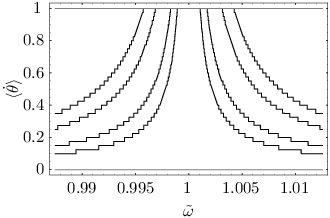
We first show numerical results for the mean tumbling rate as a function of the driving frequency . These results were obtained by a direct integration of the equations of motion (8) and (9). Fig. 8 shows the characteristic dependence on the frequency for a harmonically oscillating inverse shear rate. There is a smooth background, which is constant at low frequencies and vanishes at a high cut-off frequency. A large number of regularly ordered resonance peaks are superimposed. A qualitative discussion based on the results for time-constant shear rate can explain the general features of this plot.
4.1 Qualitative explanation
We start with some preliminary considerations, which will be confirmed analytically afterwards. As shown in section 3.3 for constant shear rates in the quasi-spherical limit, the equations of motion in regions i) and iii) and the qualitative relaxation towards the stable line in region iv) are independent of the shear rate. This behaviour remains unchanged for a time-dependent shear rate or slope parameter . Thus, the relaxation towards the stable line and the motion on the stable line are unaffected by the shear rate. As illustrated in Fig. 9, the system therefore runs on the torus with monotonously increasing angle . It moves close to the stable line into the junction region. Here it turns to one vertical side depending on the value of and reaches a neighbouring horizontal stable line. During the motion the junction region is visited over and over again periodically in time . We can label the junction with angles (, ), where
| (34) |
with integer index counts the number of visits (see Fig. 9) and is an integer multiple of counting the difference of the number of tumbling and the number of swinging motions. Starting with index , the system reaches the junction at consecutive angles , , , .
The only difference to the time-constant case of section 3 happens in the junction region ii), where the system leaves the stable line to follow the neutral line. Here, the value of the instantenous shear rate determines for the overall behaviour. Since the shear rate is now time-dependent, the slope parameter can take different signs each time the system is in the junction region and can even change signs several times within the junction region.
We first want to estimate the time the systems spends in the junction region ii) and consider corresponding limit cases of the driving frequency . Measuring time with respect to the nondimensional time , the speed of is . The time the system needs to return to the junction is of order . Since the junction region has linear dimension of the order , the time the system stays within the junction region is of the order . Thus, the fraction of time the system is within the junction region is given by the order of and the corresponding frequency is of order .
For high frequencies , the oscillation is too fast for the system to respond. Therefore the shear rate behaves effectively as a time-constant shear rate with mean slope . For a negative mean slope , there is a pure swinging motion with vanishing mean tumbling rate (see Fig. 8 b). Conversely, for a positive mean slope there is a pure tumbling motion with mean tumbling rate .
In the limit of low frequencies , the shear rate in the junction region can be regarded constant. In other words, the junction region is effectively just a point located at (, ). Each time the system is in the junction region labeled by , the sign of the slope parameter determines whether the system performs a single tumbling or a single swinging motion. The sign of depends on the initial phase , the frequency , and the index . In order to calculate the mean tumbling rate , the number of positive and negative values of , , have to be counted. Therefore, the system can be mapped on a discrete model in the low-frequency limit as shown in section 4.3). This discrete model reproduces both the constant background of the mean tumbling rate and the superimposed resonance peaks which can both be seen in Fig. 8.
For intermediate frequencies , it seems reasonable that some time-averaged slope in the junction region determines the motion of the capsule. This expectation is quantified in the next section.

4.2 Analytic solution in the junction region
The qualitative arguments of the previous section are substantiated by a full analytical investigation for a general time-dependent shear rate with parameters and close to the special point. Since we are in the quasi-spherical limit, we investigate the four regions analog to the time-constant case (sec. 3.3). The equations of motion to lowest order in remain unchanged except for the fact that the slope parameter is now time-dependent . Since the velocity in -direction in dimensionless units is , the system visits the junction labeled by (, ) at time .
As in the time-constant case (see Appendix C), there is no dependence of the solutions on the slope parameter in regions i) and iii), and no qualitative dependence on in region iv), where the trajectory merely relaxes to the next stable line. Thus, after leaving the junction region, the system moves fast towards one of the two neighbouring stable lines, before moving slowly along the stable line and returning to the junction region ii). Again, the junction region determines which stable line is chosen next, i.e. whether the capsule tumbles or swings. The corresponding first order equation of motion (C.4) in region ii) close to can be integrated for a general time-dependent as is shown in Appendix D. In the long-time limit the matched solution (D.2) in the junction region becomes asymptotically
| (35) |
where the average slope corresponding to the -th junction (, ) is defined by
| (36) |
This integral is a convolution of the time-dependent slope parameter with a Gaussian shaped kernel of width centered at . Thus, for low frequencies the kernel is effectively proportional to Dirac’s -function, while for high frequencies the kernel smoothes out the fast oscillations of . These two limit cases will be discussed in more detail in the next section.
The sign of the average slope determines whether the trajectory of the system follows the neutral vertical line along the positive (for ) or negative (for ) direction. Since the solutions in regions iii) and iv) only describe the relaxation to the next stable line, the asymptotic matching procedure then proceeds exactly as in the time-constant case. For any given time-dependent shear rate or equivalently , the sequence of average slopes at can be calculated. The mean tumbling rate is then given by
| (37) |
with the Heaviside step function . We now evaluate this expression for a specific choice of .
4.3 Harmonically oscillating shear rate
Since is periodic with period , it can be decomposed into a Fourier series consisting of an oscillation with the fundamental frequency and the corresponding higher harmonics. We constrain to a pure harmonic oscillation in the following section for simplicity. The results are easily generalised to the Fourier series of an arbitrary periodic (see Appendix E).
a)

b)

c)

d)

For a purely harmonically modulated slope
| (38) |
with mean value , amplitude , frequency and initial phase , the sequence of mean slopes can be evaluated analytically
| (39) |
where we have defined the sequence of equidistant phases
| (40) |
We now discuss the mean tumbling rate
| (41) |
as a function of , , , and .
For small modulation amplitudes , the sign of equals the sign of for all . This condition holds for all frequencies if . For , we can define a threshold frequency
| (42) |
beyond which () the phase behaviour is given by the sign of alone. The system tumbles () for and swings () for .
For large modulation amplitudes , the sign of depends on the value of the phase modulo . For phases in the region with
| (43) |
the average slopes are positive and the system performs tumbling motions and swinging motions otherwise. This behaviour is visualised in Fig. 10, where the phases modulo are interpreted as points on the circle (modulo ).
The circle consists of an arc with angle corresponding to tumbling and a complementary arc with angle corresponding to swinging. Each phase at the junction labeled by (, ) is either an element of the tumbling or an element of the swinging arc. By counting the fraction of phases within each arc the mean tumbling rate can be calculated explicitly:
- •
For an irrational frequency the values of the phases lie densely on the circle . The fraction of number of swinging to tumbling motions in the long time limit is then given by the ratio of the length and of the two intervals, leading to a mean tumbling rate of
(44) In the low frequency limit this becomes a constant .
- •
For a rational frequency with integer and coprime numbers and the phases lie on equidistant phases (with ) on the circle . In the long time limit, all of these angles are visited equal amounts of times. The ratio of number of swinging to tumbling motions is given by the ratio of number phases in the two intervals of length and . For high values of , approximately phases lie within the interval . Then the mean tumbling rate is approximately given by the expression (44) valid for irrational frequencies. For low denominators , the number of phases within the two intervals additonally depends upon the initial phase . An integer frequency for instance gives a tumbling rate of either or depending only on the initial condition. For a general rational frequency, counting the number of phases in the tumbling sector gives
(45) with given by eqn. (43). Here, and are the floor and ceiling functions, which denote the closest integer smaller or larger than the argument, respectively.
Plotting the mean tumbling rate over small frequencies in Fig. 8, we can identify a smooth irrational background (44) superimposed by rational peaks (45). Their amplitudes depends on the denominator and the initial phase . For integer resonance frequencies, the peaks go either to or .
a)
b)

Mathematically speaking, the peaks at rational frequencies are infinitesimally narrow. Since experiments and numerical methods run only for a finite time, the peaks are broadened to a finite width, which can be estimated in the following for the most dominant peaks with nearly integer frequency
| (46) |
Let us assume that , so that the system tumbles with (for ). For exactly integer modulation frequency , the phase stays constant for all . For a non-integer frequency the -th phase modulo is . If this phase does not change by more than by the width of the tumbling arc during the simulation time , the system stays in the tumbling regime. Therefore we can estimate the width of the integer resonance peaks as
| (47) |
This result is confirmed in Fig. 11, where numerically evaluated peak widths are compared to expression (47) for different modulation amplitudes . For the numerical data, the peak width was defined to be the frequency interval in which the mean tumbling rate during the simulation time was larger than . The agreement is excellent.
4.4 Dynamic phase diagram
We summarise our findings in a dynamic phase diagram. While the specific shape of the phase diagram depends on the particular functional time-dependence of the shear flow, the general features hold for any oscillating time-dependent flow with mean inverse shear rate and oscillation amplitude , compare eqn. (31). From our study of time-constant shear flow we know the location of the phase boundary . In Fig. 12, a grey scale plot of the mean tumbling rate is shown as a function of the oscillation amplitude relative to the distance of the mean shear rate to the phase boundary, , versus the oscillation frequency measured im units of the mean shear rate. The colour level indicates the mean tumbling rate as defined in eqn. (10) for finite simulation times, black colour indicating a swinging motion . In Fig. 12, a mean shear rate in the swinging regime (for constant flow) was chosen, . One can see that for oscillation amplitudes below the distance to the phase boundary, , the capsule never tumbles. In order to induce tumbling motion, the instantaneous shear rate has to cross the phase boundary. For higher modulation frequencies, the oscillation amplitude threshold for tumbling is even higher and given by
| (48) |
Above the oscillation amplitude threshold the mean tumbling rate grows continuously on the irrational background with increasing amplitude. At the resonance frequencies the mean tumbling rate reaches values given by eqn. (45).

5 Conclusions
We have investigated the motion of microcapsules in time dependent shear flow in a reduced model. The equations of motions were studied analytically in the quasi-spherical limit for constant viscosity contrast. We have identified the stable and unstable fixed points at lowest order in the deformation, which lead to swinging and tumbling limit cycles at first order depending on the shear rate. Close to the dynamic phase boundary, the expansion of the equations of motion was carried out to first order in the deformation. Their analytic solution was facilitated by solving the trajectories in different regions in phase space separately: One region close to the stable fixed points with comparatively slow dynamics, one region close to the unstable fixed points with a comparatively fast motion, and a junction close to the neutral fixed point, which also acts on a fast time scale. The direction of the dynamics in this latter region is determined by the value of the shear rate. The analytic inner solutions for the trajectories were then joined together using the method of matched asymptotic expansion.
As a central result of this study, we now fully understand the dynamic phase behaviour of quasi-spherical capsules in time-independent shear flow and have determined the phase boundary between swinging and tumbling as a function of shear rate and viscosity as . In physical parameters the phase boundary reads
| (49) |
We then generalised our result to time-dependent shear rates. The equations of motion were integrated analytically in the different dynamic regions. Again, we found that the motion for one period is determined by a weighted time-average of the shear rate during the time when the system is close to the junction. We have thus mapped the continuous capsule dynamics to a discrete model valid for all time-dependent flows. Our general results were then applied to harmonically modulated shear rates around a finite mean value, where the dynamic phase diagram was constructed explicitly. As the dynamics is determined by the (time-averaged) value of the shear rate at specific times only, the system shows a pronounced resonance behaviour: By choosing suitable modulation frequencies, it is possible to induce tumbling motion for capsules, which would otherwise swing at constant mean shear rate. The width of the resonance peaks for finite simulation time can also be expressed analytically. For not resonant frequencies, the mean tumbling rate is determined by an analytic expression, which vanishes beyond an upper modulation frequency threshold. The agreement of numerical solutions of the original equations of motion with the theoretical results is excellent.
In summary, we have reached a fairly complete analytical understanding of the motion of a quasi-spherical capsule in time-dependent shear flow. In the course of the study, we have also obtained analytical expressions for capsules in constant shear flow whose equations of motion previously have been studied merely numerically.
Acknowledgements.
Financial support of the DFG with in the priority programme SPP 1164 “Nano- and Microfluidics” is gratefully acknowledged.Appendix A Keller-Skalak quantities
Appendix B Notation for asymptotic limits
We use the following conventions, where and are real functions of the real variable , is a real constant and and are real numbers:
| (B.1) | |||
| (B.2) | |||
| (B.3) |
Appendix C Asymptotic matching for time-constant shear rates
Here, we describe our analytical procedure for obtaining the asymptotic trajectory of the limit cycle in the quasi-spherical case when the system is close to the special point and . For each of the four regions of Fig. 6, the quasi-spherical equation of motion (28) is solved asymptotically, compare Fig. 7.
- i)
, : Expansion gives the equation of motion
(C.1) which is independent of the shear rate, i.e. independent of the slope . Its solution is given by
(C.2) where is an arbitrary point on the trajectory. This solution will be used to match with the solution of region ii). As can be seen in iv) by closing the trajectory on the torus, the limit cycle in region i) is simply given by the original stable line
(C.3) Thus, to leading order in , the system runs on the stable line with . Even when the system starts off the limit cycle, the stable character of and leads to a fast relaxation towards the stable line, while the angle changes slowly due to . Therefore, the matching with region ii) will not depend on the initial point and the general solution (C.2) is independent of the slope parameter .
- ii)
, : Here, stable and neutral line meet, and the expansion gives
(C.4) In this region, the vector field corresponding to is small enough for the finite but small value of to have a significant influence on the the vector field and thus on the motion. Here, the exact value of the the shear rate or the slope parameter is critical as can be seen by the solution
(C.5) which has been matched with the general solution (C.2) of region i) and which is independent of the initial point. Here, we use the error function
(C.6) Thus, the sign of determines the sign of . For negative the neutral line with is choosen which leads to a swinging motion. Conversely, for a positive the neutral line with is choosen, corresponding to a tumbling motion (see region iii)). Region ii) with acts as a junction which only depends on the sign of the slope parameter .
- iii)
In the region and close to the neutral line, the expansion gives a slope-independent equation of motion
(C.7) whose matched solution
(C.8) depends on the slope parameter . This solution describes the relaxation towards the next stable line which has been chosen in region ii).
- iv)
In the region and , where neutral and unstable lines meet again, the expansion gives
(C.9) with matched solution
(C.10) where we used the imaginary error function
(C.11) The upper and lower signs depend on which neutral line was chosen in region ii). Although both the equation of motion and the solution depend on , the system relaxes toward the stable line for all values of . It then starts over again in region i) close to the stable line. By matching with the general solution of region i) the trajectory closes and the solution (C.3) is obtained.
Appendix D Asymptotic matching for time-dependent shear rates
Appendix E Fourier series
The oscillating part of any general period slope (see eqn. (31)) can be uniquely decomposed into a Fourier series
| (E.1) |
In this case, the sequence of mean slopes (see eqn. (36)) is explicitly given by the Fourier series
| (E.2) |
For and for all , we recover eqn. (39). The amplitude is damped by the factor .
References
- Eggleton and Popel (1998) C. D. Eggleton and A. S. Popel, Phys. Fluids 10, 1834 (1998).
- Walter et al. (2001) A. Walter, H. Rehage, and H. Leonhard, Colloid Surf. A 183-185, 123 (2001).
- Fischer (2004) T. M. Fischer, Biophys. J. 86, 3304 (2004).
- Abkarian et al. (2007) M. Abkarian, M. Faivre, and A. Viallat, Phys. Rev. Lett. 98, 188302 (2007).
- Fischer (2007) T. M. Fischer, Biophys. J. 93, 2553 (2007).
- Barthès-Biesel (1980) D. Barthès-Biesel, J. Fluid Mech. 100, 831 (1980).
- Barthès-Biesel and Rallison (1981) D. Barthès-Biesel and J. M. Rallison, J. Fluid Mech. 113, 251 (1981).
- Keller and Skalak (1982) S. R. Keller and R. Skalak, J. Fluid Mech. 120, 27 (1982).
- Barthes-Biesel and Sgaier (1985) D. Barthes-Biesel and H. Sgaier, J. Fluid Mech. 60, 119 (1985).
- Barthès-Biesel et al. (2002) D. Barthès-Biesel, A. Diaz, and E. Dhenin, J. Fluid Mech. 460, 211 (2002).
- Lac et al. (2004) E. Lac, D. Barthès-Biesel, N. A. Pelekasis, and J. Tsamopoulos, J. Fluid Mech. 516, 303 (2004).
- Lac and Barthès-Biesel (2005) E. Lac and D. Barthès-Biesel, Phys. Fluids 17, 72105 (2005).
- Finken and Seifert (2006) R. Finken and U. Seifert, J. Phys.: Condens. Matter 18, L185 (2006).
- Skotheim and Secomb (2007) J. M. Skotheim and T. W. Secomb, Phys. Rev. Lett. 98, 078301 (2007).
- Pozrikidis (1995) C. Pozrikidis, J. Fluid Mech. 297, 123 (1995).
- Ramanujan and Pozrikidis (1998) S. Ramanujan and C. Pozrikidis, J. Fluid Mech. 361, 117 (1998).
- Noguchi and Gompper (2005) H. Noguchi and G. Gompper, Proc. Natl. Acad. Sci. U. S. A. 102, 14159 (2005).
- Kessler et al. (2007) S. Kessler, R. Finken, and U. Seifert, J. Fluid Mech. 605, 207 (2007).
- Sui et al. (2008a) Y. Sui, H. T. Low, Y. T. Chew, and P. Roy, Phys. Rev. E 77, 016310 (2008a).
- Sui et al. (2008b) Y. Sui, Y. T. Chew, P. Roy, Y. P. Cheng, and H. T. Low, Physics of Fluids 20, 112106 (2008b).
- Dodson III and Dimitrakopoulos (2008) W. R. Dodson III and P. Dimitrakopoulos, Phys. Rev. Lett. 101, 208102 (2008).
- Kraus et al. (1996) M. Kraus, W. Wintz, U. Seifert, and R. Lipowsky, Phys. Rev. Lett. 77, 3685 (1996).
- de Haas et al. (1997) K. H. de Haas, C. Blom, D. van den Ende, M. H. G. Duits, and J. Mellema, Phys. Rev. E 56, 7132 (1997).
- Seifert (1999) U. Seifert, Eur. Phys. J. B 8, 405 (1999).
- Pozrikidis (2001) C. Pozrikidis, J. Fluid Mech. 440, 269 (2001).
- Noguchi and Gompper (2004) H. Noguchi and G. Gompper, Phys. Rev. Lett. 93, 258102 (2004).
- Kantsler and Steinberg (2005) V. Kantsler and V. Steinberg, Phys. Rev. Lett. 95, 258101 (2005).
- Kantsler and Steinberg (2006) V. Kantsler and V. Steinberg, Phys. Rev. Lett. 96, 036001 (2006).
- Misbah (2006) C. Misbah, Phys. Rev. Lett. 96, 28104 (2006).
- Vlahovska and Gracia (2007) P. M. Vlahovska and R. S. Gracia, Phys. Rev. E 75, 016313 (2007).
- Lebedev et al. (2007) V. V. Lebedev, K. S. Turitsyn, and S. S. Vergeles, Phys. Rev. Lett. 99, 218101 (2007).
- Pozrikidis (2003) C. Pozrikidis, Modelling and simulation of capsules and biolocical cells (Chapman & Hall/CRC, 2003).
- Mohandas and Evans (1994) N. Mohandas and E. Evans, Annu. Rev. Biophys. Biomolec. Struct. 23, 787 (1994).
- Kantsler et al. (2007) V. Kantsler, E. Segre, and V. Steinberg, Phys. Rev. Lett. 99, 178102 (2007).
- Noguchi et al. (2008) H. Noguchi, G. Gompper, L. Schmid, A. Wixforth, and T. Franke, arXiv:0811.0862v1 (2008).
- Hinch (1991) E. J. Hinch, Perturbation Methods (Cambridge University Press, 1991), chap. 5.