The Josephson light-emitting diode

Electron-hole recombination in semiconductors accompanied by emission of visible light is a key element of many technologies. Semiconducting QDs have been proposed to enhance these technologies by engineering the frequencies of radiation [1]. In the context of modern research, they have been considered as a controllable source of single [2, 3, 4] and entangled two-photon pairs [5, 6]. QDs allow for integration of photon-based technologies and solid state systems where electronic degrees of freedom are used to represent quantum information (e.g. electron spins in quantum dots (QDs) [7], charge- [8] and flux qubits [9] in superconducting (SC) circuits), combining the advantages of both. For quantum information purposes, it is crucial that indistinguishable optical photons or pairs of photons can be created on demand. The semiconducting QDs provide means to achieve this [10].

SC Josephson junctions can also be a source of coherent radiation. When the junction is biased with a voltage $V_{\rm sd}$, photons with frequency $\omega=2eV_{\rm sd}/\hbar$ are emitted corresponding to Cooper pair transfers between the two SC leads. This radiation is coherent since the Cooper pair transfers are coherent owing to macroscopic phase coherence of SC condensates involved [11]. The frequency of Josephson radiation is limited by the SC energy gap $\Delta\sim$ 1 meV, $\hbar\omega=2eV_{\rm sd}<4\Delta$. This is three orders of magnitude away from the optical frequency range.

Many theoretical predictions (e.g. [12]) promote the combination of SCs and semiconductors within a single nanostructure. This difficult technological problem attracted attention for a long time [13]. Recent progress has been achieved with semiconductor nanowires. SC field-effect transistor [14] and Josephson effect [15] in a semiconducting QD have been experimentally confirmed.

In this Letter, we propose and investigate theoretically a setup where a superconducting p-n junction enclosing a semiconducting QD emits photons in the optical range, see Fig. 1. This device is biased by a voltage $V_{\rm sd}$ which is close to the semiconducting band gap. We show that, owing to SC correlations, the device emits the photons in the frequency range $eV_{\rm sd}/\hbar$ concentrated in several discrete spectral lines, the line-width being restricted by the emission time only. The acts of photon emission correlate. In this way, one can arrange emmision of pairs of photons of opposite polarization. The device is also shown to emit in the frequency range $2eV_{\rm sd}/\hbar$. The emitted light is associated with Cooper pair transfer between the SC leads and is therefore coherent. This is in fact Josephson radiation at optical frequency.

Setup details. The semiconducting QD encompasses two levels: one for electrons(e), one for holes(h). The levels are coupled to corresponding SC leads (source and drain), those being characterized by energy gaps $\Delta_{e,h}$. The levels are aligned to the corresponding chemical potentials $\mu_{e,h}$. We count their energies $E_{e,h}$ from these potentials assuming $|E_{e,h}|\ll|\Delta_{e,h}|$. The tunnel coupling in the normal state is characterized by the broadening of a corresponding level, $\Gamma_{{\rm t};e,h}$, those being proportional to squares of the tunneling amplitudes. In the presence of superconductivity, we treat the coupling to the SC leads in second order perturbation theory [16]. This accounts for coherent transfers of electron singlets between the QD and the SC leads, and amounts to an induced pair potential for the level, with ${\tilde{\Delta}}_{e,h}=(1/2)\exp[i\phi_{e,h}]\Gamma_{{\rm t};e,h}$ (assuming $\Gamma_{{\rm t};e,h}\ll|\Delta_{e,h}|$, [12]), and $\phi_{e,h}$ the phase of the corresponding $\Delta_{e,h}$.

The induced pair potential results in formation of four discrete low-energy states at each (electron or hole) side of the setup. We write the effective low-energy Hamiltonian for electron side, skipping index “e” for $\tilde{\Delta}$, $\Gamma$, $E$,

where we assume that the charging energy (repulsive on-site interaction) $U\ll|\Delta|$.

By diagonalizing ${\widetilde{H}}_{D}^{e}$, we obtain two degenerate single-particle states $|\uparrow\rangle=c_{\uparrow}^{\dagger}|0\rangle$ and $|\downarrow\rangle=c_{\downarrow}^{\dagger}|0\rangle$ with energy $E$ forming a doublet ($|0\rangle$ denotes the empty level), and two singlets, those being linear superpositions of $|0\rangle$ and $|2\rangle=c_{\uparrow}^{\dagger}c_{\downarrow}^{\dagger}|0\rangle$. For the ground state singlet, we obtain

with energy $\varepsilon_{g}={\tilde{E}}-({\tilde{E}}^{2}+|{\tilde{\Delta}}|^{2})^{1/2}$, (${\tilde{E}}=E+(U/2)$). The coherence factors [17] are $|u|,|v|=(1/\sqrt{2})[1\pm{\tilde{E}}/({\tilde{E}}^{2}+|{\tilde{\Delta}}|^{2})^{1/2}]^{1/2}$. The excited state singlet reads

with energy $\varepsilon_{ex}={\tilde{E}}+({\tilde{E}}^{2}+|{\tilde{\Delta}}|^{2})^{1/2}.$ Similary, four states are formed on the hole side of the setup. Since we are dealing with holes, we define the corresponding vacuum $|0\rangle_{h}$ as the level occupied by two electrons [16]. Apart from this difference, the energies and wave functions of the states are given by above expressions with $E,\tilde{\Delta},\Gamma_{\rm t},U=E_{h},\tilde{\Delta}_{h},\Gamma_{{\rm t};h},U_{h}$. One could easily include the interaction energy between electrons and holes in the above scheme. We neglect this interaction since we do not expect it to change our results qualitatively.

A SC p-n junction has been discussed in [18], and supplemented with a QD in [19], in the context of superradiance which is irrelevant for our proposed effects.

Emission of “red” light. So far, we have not enabled charge transfer through the setup. This can only proceed by recombination of an electron and a hole at different sides of the setup, see Fig. 1. Such transfer has to dispose an energy $\simeq eV_{\rm sd}$ corresponding the energy difference between the electron and hole level, and therefore is accompanied by emission of a photon of this energy: Let us call it “red” photon. The recombination is described by the following Hamiltonian:

The time dependence $\exp(\pm ieV_{{\rm sd}}t)$ accounts for the difference between $\mu_{e}$ and $\mu_{h}$. Eq. (4) is a minimal model for the photon-assisted recombination of e-h pairs. We assume usual selection rules [20] implying that the holes are “heavy”, $h^{\dagger}_{\uparrow}$ ($h^{\dagger}_{\downarrow}$) creates a hole with the total angular momentum $j_{z}=3/2(-3/2)$. Eq. (4) then ensures the conservation of total angular momentum: The polarization ($p=\pm$) of the photon emitted into a mode $q$ ($a^{\dagger}_{q,\pm}$) is determined by the electron and hole spins [21]. An isolated QD in the state $|\uparrow\rangle_{e}|\downarrow\rangle_{h}$ would recombine to $|0\rangle_{e}|0\rangle_{h}$ with the rate $\Gamma_{\rm ph}\propto G^{2}$. Since the states of the QD are modified by coupling to SC leads [see Eqs. (2),(3)], the “red” emission causes transitions between all QD states (see also Fig. 2a)).

An even parity emission cycle (EP) ($\#e+\#h$=even) and an odd parity (OP) cycle ($\#e+\#h$=odd) exist. The transitions proceed between the discrete states of the QD (see Fig. 2a)). They give rise to sharp emission lines with frequencies directly related to energy differences between the states [22]. The rates incorporate the coherence factors, for instance,

EP and OP cycles are connected by transitions of a second type which involve the excitation of a single quasiparticle with energy $>\Delta_{e,h}$ in one of the leads [16] and therefore change the parity that is conserved in course of photon emission. They give rise to a continuous spectrum of the “red” light emitted that is separated from the lines by frequency ${\rm min}(\Delta_{e},\Delta_{h})/\hbar$. The transition rates of the second type are smaller as those of the first type by a typical reduction factor $|\tilde{\Delta}|/|\Delta|\ll 1$.

The emission intensity $i(\omega)=\sum_{ab,p}w^{p}_{a\rightarrow b}(\omega)\rho_{a}$ of the QD can be computed from the probabilities $\rho_{a}$ to be in one of 16 possible QD states $|a\rangle$. They follow from the stationary solution of the master equation describing the setup dynamics, governed by the rates $W_{a\rightarrow b}^{p}=\int d\omega^{\prime}\,w_{a\rightarrow b}^{p}(\omega^{\prime})$ [16]. 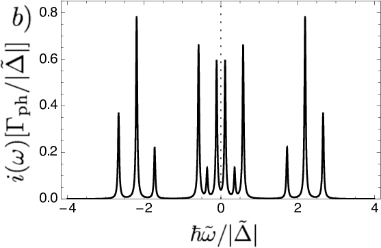The emission intensity computed is shown in Fig. 3 versus photon frequency $\omega$ (we assume for simplicity that $|{\tilde{\Delta}}_{e}|=|{\tilde{\Delta}}_{h}|$ and $U_{e}=U_{h}$). Plot a) gives the intensity at the scale $|\hbar\omega-eV_{\rm sd}|\sim|\Delta|$ (for the case $E_{e}=E_{h}=U=0$). Three discrete peaks are visible at much smaller scale of the induced gap $|\hbar\omega-eV_{\rm sd}|\sim|\tilde{\Delta}|$. At $\hbar\omega\approx eV_{\rm sd}-|\Delta|$, a continuous tail of emission starts (enlarged in the inset) reflecting quasiparticle creation in the leads. The dashed line is the emission spectrum of the same QD without superconductivity. In this case, the spectrum is continuously broadened on the scale $\Gamma_{\rm t}=2|\tilde{\Delta}|$. The total emission intensity approximately corresponds to the total intensity of the three discrete lines in the SC case. Plot b) illustrates the regime of photon-pair emission. The chosen parameters $E_{e}=1.9$, $E_{h}=-1.6$ and $U=0.28$ (in units of $|{\tilde{\Delta}}|$) induce a large population of the ground state singlet $|g\rangle_{e}|\rangle g\rangle_{h}$ ($\rho_{gg}\simeq 0.75$, $|u_{e}|\sim 0.97$ and $|v_{h}|\sim 0.96$).

This has striking consequences for the cascade emission process $|g\rangle_{e}|g\rangle_{h}\rightarrow|1\rangle_{e}|1\rangle_{h}\rightarrow|g\rangle_{e}|g\rangle_{h}$ shown in b) (main full lines). From Eqs. (5) and (6) we deduce, that $W_{|g\rangle_{e}|g\rangle_{h}\rightarrow|1\rangle_{e}|1\rangle_{h}}^{p}/W_{|1\rangle_{e}|1\rangle_{h}\rightarrow|g\rangle_{e}|g\rangle_{h}}^{p^{\prime}}=|v_{e}u_{h}/u_{e}v_{h}|^{2}\ll 1$. Therefore, this process produces two-photons of opposite polarization in a pair (i.e. the delay time between the emission of the first and second photon is much shorter than the emission time of the pair) and with energies $\hbar\omega=eV_{\rm sd}\pm(\varepsilon_{g}^{e}+\varepsilon_{g}^{h}-E_{e}-E_{h})$. We point out that the energies of these correlated photons are different, however, the polarization and energy of the photons are uncorrelated. This cascade corresponds to the biexciton-exciton decay discussed in [5] in the context of polarization-entangled photons. Therefore, potentially pairwise entangled photons [23] could be identified efficiently in the time domain. The dotted lines (OP cycle) are energetically distinct from the full lines (EP cycle) as a consequence of induced $|{\tilde{\Delta}}|$ and $U$. This allows us to distinguish emission processes from different cycles. We remark that the charge current through the device just equals the emission intensity of “red” photons.

Emission of “blue” light at $2eV_{\rm sd}$. We now consider the emission of a single-photon per Cooper pair transfer through the QD. Since the Cooper pair charge is $2e$, the energy associated with its transfer is $2eV_{\rm sd}$. If a single photon is emitted by this process, it must have a frequency $\sim 2eV_{\rm sd}/\hbar$ which we call a “blue” photon. Since only one electron-hole pair recombines radiatively in the emission process, we need a static in-plane electric field ${\bm{E}}_{0}$ that annihilates the other pair (see Fig. 2b)). This annihilation without emission is described by

with $V_{0}^{\pm}\propto E_{0,x}\mp iE_{0,y}$. To second order in the total interaction Hamiltonian $H_{\rm int}=H_{\rm int,1}+H_{\rm int,0}$, the rate to emit a single “blue” photon (with polarization $p=\pm$) is $W_{a\rightarrow b}^{p}=(2\pi/\hbar)|{\cal A}_{a\rightarrow b}^{p}|^{2}\delta(\varepsilon_{b}-\varepsilon_{a}+\hbar\omega-2eV_{\rm sd})$ between initial state $|a\rangle$ (with energy $\varepsilon_{a}$) and final state $|b\rangle$ (with energy $\varepsilon_{b}$) of the QD.

For the case where $|a\rangle$ and $|b\rangle$ belong to the singlet subspace [24], we obtain (in leading order in $1/eV_{\rm sd}$),

We note that the amplitude can also connect different initial and final QD states resulting in incoherent photons. However, they are emitted at different frequencies. The light emitted at $\hbar\omega=2eV_{\rm sd}$ is always coherent. In this case, ${\cal A}_{a\rightarrow b}^{p}={\cal A}_{a\rightarrow a}^{p}\equiv{\cal A}_{a}^{p}$ and $\langle a|00\rangle\langle 22|a\rangle=\pm\exp[i(\phi_{e}-\phi_{h})]|u_{e}u_{h}v_{e}v_{h}|$. The “blue” emission out of the doublet states $|\uparrow\rangle_{e}|\downarrow\rangle_{h}$ and $|\downarrow\rangle_{e}|\uparrow\rangle_{h}$ is anomalously small with ${\cal A}_{a\rightarrow b}^{p}\propto(eV_{\rm sd})^{-3}$ and is irrelevant.

Let us consider two QDs embedded in a SQUID loop as shown in Fig. 4a). Coherent emission from either QD (1 or 2) into a common photonic mode (and with the same polarization) has amplitudes ${\cal A}_{1,a}^{p}$ and ${\cal A}_{2,a^{\prime}}^{p}$ (assuming the QDs are in states $|a\rangle$ and $|a^{\prime}\rangle$, resp.). The total intensity $I_{J}$ of photons in the common mode is proportional to $\sum_{aa^{\prime},p}\rho_{a}\rho_{a^{\prime}}|{\cal A}_{1,a}^{p}e^{i2\pi l_{1}/\lambda_{J}}+{\cal A}_{2,a^{\prime}}^{p}e^{i2\pi l_{2}/\lambda_{J}}|^{2}$, where $\lambda_{J}=hc/2eV_{\rm sd}$ is the wave length of coherent light at the Josephson frequency and $l_{1}$ and $l_{2}$ are the respective path lengths from the QDs to the detector. The interference contribution is proportional to $\sum_{aa^{\prime},p}\rho_{a}\rho_{a^{\prime}}{\rm Re}[{\cal A}_{1,a}^{p}({\cal A}_{2,a^{\prime}}^{p})^{*}]$ with ${\rm Re}[{\cal A}_{1,a}^{p}({\cal A}_{2,a^{\prime}}^{p})^{*}]\propto\cos[2\pi((l_{1}-l_{2})/\lambda_{J}+\Phi/\Phi_{0})]$, where we use that $\phi_{1e}-\phi_{1h}-(\phi_{2e}-\phi_{2h})=2\pi\Phi/\Phi_{0}$, with $\Phi$ the flux through the SQUID and $\Phi_{0}=hc/2e$ the SC flux quantum.

Fig. 4b) shows the computed emission intensity of $2eV_{\rm sd}$ photons as a function of flux $\Phi$. We find that the intensity oscillates with period given by the superconducting flux quantum $\Phi_{0}=hc/2e$, and has a magnitude of order $(\Gamma_{\rm ph}/\hbar)Q$ with $Q\equiv 2|V_{0}^{p}{\tilde{\Delta}}|^{2}/(eV_{\rm sd})^{4}=2|{\bm{d}}\cdot{\bm{E}}_{0}|^{2}|{\tilde{\Delta}}|^{2}/(eV_{\rm sd})^{4}$, where ${\bm{d}}$ is the optical dipole moment [16] of the QD [25]. The electric field ${\bm{E}}_{0}$ could be created by gates. Typical critical field strengths before quenching the photoluminescence of optical QDs are on the order of several Volts/$\mu$m [26]. Taking $|{\bm{d}}_{\ ||}|$ on the order of the QD diameter $\sim 20$ nm and estimating $|\tilde{\Delta}|\lesssim 1$ meV (bounded by $|\Delta|$), we arrive at an intensity $I_{J}\sim$ 4 photons/s assuming $eV_{\rm sd}\sim 1$eV and $\hbar/\Gamma_{\rm ph}\sim$ 0.1 ns at $2eV_{\rm sd}$. This intensity is measurable with single-photon detectors [27]. In addition, the Purcell effect in a QD-cavity system could enhance $\Gamma_{\rm ph}$ substantially [28].

In conclusion, we investigated emission from a quantum dot (QD) embedded in a superconducting (SC) p-n junction. The presence of SC leads induces an effective pair-potential for electrons (e) and holes (h) on the QD. At frequencies $\omega$ close to the voltage bias $eV_{\rm sd}/\hbar$ of the p-n junction, a regime exists where radiation is correlated in pairs of oppositely polarized photons. At $\omega=2eV_{\rm sd}/\hbar$, emission is associated with Cooper pair transfer and is coherent. We proposed an experiment where interference of radiation from distant QDs arranged in a SQUID geometry can be manipulated by a magnetic flux. This provides a fascinating new tool to manipulate coherent light at optical frequencies.

We acknowledge useful discussions with N. Akopian, C.W.J. Beenakker, S. Frolov, D. Loss, U. Perinetti, and V. Zwiller and financial support from the Dutch Science Foundation NWO/FOM.