Connectivity, Percolation, and Information Dissemination in Large-Scale Wireless Networks with Dynamic LinksThanks: This research is supported in part by National Science Foundation (NSF) Cyber Trust grant CNS-0716335, and by Army Research Office (ARO) grant W911NF-07-1-0524.Thanks: The material in this paper was presented in part at the 27th IEEE Conference on Computer Communications (INFOCOM), Phoenix, AZ, April 2008.Thanks: Z. Kong and Edmund M. Yeh are with the Department of Electrical Engineering, Yale University (email: zhenning.kong@yale.edu, edmund.yeh@yale.edu)

Zhenning Kong Edmund M. Yeh Affiliation:

Abstract

We investigate the problem of disseminating broadcast messages in wireless networks with time-varying links from a percolation-based perspective. Using a model of wireless networks based on random geometric graphs with dynamic on-off links, we show that the delay for disseminating broadcast information exhibits two behavioral regimes, corresponding to the phase transition of the underlying network connectivity. When the dynamic network is in the subcritical phase, ignoring propagation delays, the delay scales linearly with the Euclidean distance between the sender and the receiver. When the dynamic network is in the supercritical phase, the delay scales sub-linearly with the distance. Finally, we show that in the presence of a non-negligible propagation delay, the delay for information dissemination scales linearly with the Euclidean distance in both the subcritical and supercritical regimes, with the rates for the linear scaling being different in the two regimes.

I Introduction

Large-scale wireless networks for the gathering, processing, and dissemination of information have become an important part of modern life. To ensure that important broadcast messages can be received by each node in a wireless network, the network needs to maintain full connectivity [1]. Here, the system ensures that each pair of network nodes are connected by a path of consecutive links. In large-scale wireless networks exposed to severe natural hazards, enemy attacks, and resource depletion, however, the full connectivity criterion may be overly restrictive or impossible to achieve. In these challenging environments, the system designer may reasonably aim for a slightly weaker notion of connectivity, one which ensures that a high fraction of the network nodes can successfully receive broadcast messages. This latter viewpoint can be explored using the mathematical theory of percolation [2, 3, 4, 5].

In this paper, we investigate the problem of information dissemination in wireless networks from a percolation-based perspective. Using a model of wireless networks based on random geometric graphs with dynamic on-off links, we show that the delay for disseminating broadcast information exhibits a phase transition as a function of the underlying node density. Assuming zero propagation delay, we show that in the subcritical regime, the delay scales linearly with the distance between the sender and receiver. In the supercritical regime, the delay scales sub-linearly with the distance.

In recent years, percolation theory, especially continuum percolation theory [4, 5], has become a useful tool for the analysis of large-scale wireless networks [6, 7, 8, 9, 10, 11, 12, 13, 14, 15]. A major focus of continuum percolation theory is the random geometric graph in which nodes are distributed according to a Poisson point process with constant density $\lambda$ , and two nodes share a link if they are within distance 1 of each other. A fundamental result of continuum percolation concerns a phase transition effect whereby the macroscopic behavior of the random geometric graph is very different for densities below and above the critical density $\lambda_{c}$ . For $\lambda<\lambda_{c}$ (subcritical), the connected component containing the origin contains a finite number of points almost surely. For $\lambda>\lambda_{c}$ (supercritical), the connected component containing the origin contains an infinite number of points with a positive probability [3, 4, 5].

Wireless networks are subject to multi-user interference, fading, and noise. Thus, even when two nodes are within each other’s transmission range, a viable communication link may not exist [7]. Furthermore, due to fading, the link quality can vary dynamically in time, inducing a frequently changing network topology. To capture these effects, we model a wireless network by a random geometric graph in which each link’s functionality (activity) varies dynamically in time according to a Markov on-off process. Using this model, we investigate the problem of disseminating broadcast messages in wireless networks. Due to the dynamic on-off behavior of links, a delay is incurred in transmitting a broadcast message from the sender to the receiver even when propagation delay is ignored. The main question we address is how this delay scales with the distance between the sender and the receiver.

As a first step, we show that the connectivity of the network with dynamic links exhibits a phase transition as a function of the underlying node density. We characterize the critical density for this phase transition in terms of the link state process. Next, we show that the delay for disseminating broadcast information exhibits two behavioral regimes, corresponding to the phase transition of the underlying network connectivity. When the dynamic network is in the subcritical phase, ignoring propagation delays, the delay scales linearly with the Euclidean distance between the sender and the receiver. This follows from the fact that in this regime, connectivity decays exponentially with distance, and on average, any information dissemination process is blocked by inactive links after the message travels a finite distance (and is resumed after the next link turns back on). When the dynamic network is in the supercritical phase, the delay scales sub-linearly with the distance between the sender and the receiver. In this case, the delay is determined largely by the amount of time it takes for the message to reach the infinite connected component of the dynamic network. Finally, we characterize the delay for information dissemination when propagation delays are taken into account. Here, the problem becomes more subtle. We show that, with the presence of a non-negligible propagation delay, the delay for information dissemination scales linearly with the Euclidean distance between the sender and the receiver in both the subcritical and supercritical regimes, with the rates for the linear scaling being different in the two regimes.

In order to study the behavior of information dissemination delay in wireless networks with dynamic links, we model the problem as a first passage percolation process [16, 17]. Similar first passage percolation problems have been studied within the context of lattices [3, 16]. Related continuum models are considered in [17, 8, 13]. In [17], Deijfen studies a continuum growth model for a spreading infection with Poisson point processes, and shows that the shape of the infected cluster scales linearly with time in all directions. In [8], Dousse et al. study how the latency of information dissemination scales within an independent site percolation model in wireless sensor networks. There, each sensor independently switches between the on and off states at random from time to time. The authors show that the latency scales linearly with the distance between the sender and the receiver when the dynamic sensor network is in the subcritical phase. In [13], the authors obtain similar results for degree-dependent site percolation model in wireless sensor networks. Unlike the problems studied in [8, 13], however, the problem addressed in this paper requires a bond percolation model, which demands different modelling and analysis techniques. Furthermore, in contrast to [17, 8], we also study the delay scaling for networks in the supercritical phase. Finally, we present new results regarding networks with propagation delay.

The remainder of this paper is organized as follows. In Section II, we outline some preliminary results for random geometric graphs and continuum percolation. In Section III, we present a simple model for wireless networks with static unreliable links. In Section IV, we introduce a more sophisticated model for wireless networks with dynamic unreliable links, and present our main results regarding percolation-based connectivity and information dissemination within this model. In Section V, we present simulation results, and finally, in Section VI, we conclude the paper.

II Random Geometric Graphs and Continuum Percolation

II-A Random Geometric Graphs

We use random geometric graphs to model wireless networks. That is, we assume that the network nodes are randomly placed over some area or volume, and a communication link exists between two (randomly placed) nodes if the distance between them is sufficiently small, so that the received power is large enough for successful decoding. A mathematical model for this is as follows. Let $\|\cdot\|$ be the Euclidean norm, and $f(\cdot)$ be some probability density function (p.d.f.) on $\mathbb{R}^{d}$ . Let ${\mathbf{X}}_{1},{\mathbf{X}}_{2},...,{\mathbf{X}}_{n}$ be independent and identically distributed (i.i.d.) $d$ -dimensional random variables with common density $f(\cdot)$ , where ${\mathbf{X}}_{i}$ denotes the random location of node $i$ in $\mathbb{R}^{d}$ . The ensemble of graphs with undirected links connecting all those pairs $\{{\mathbf{x}}_{i},{\mathbf{x}}_{j}\}$ with $\|{\mathbf{x}}_{i}-{\mathbf{x}}_{j}\|\leq r,r>0,$ is called a random geometric graph [5], denoted by $G({\cal X}_{n},r)$ . The parameter $r$ is called the characteristic radius.

In the following, we consider random geometric graphs $G({\cal X}_{n},r)$ in $\mathbb{R}^{2}$ , with ${\mathbf{X}}_{1},{\mathbf{X}}_{2},...,{\mathbf{X}}_{n}$ distributed i.i.d. according to a uniform distribution in a square area ${\cal A}=[0,\sqrt{\frac{n}{\lambda}}]^{2}$ . Let $A=|{\cal A}|$ be the area of ${\cal A}$ . There exists a link between two nodes $i$ and $j$ if and only if $i$ lies within a circle of radius $r$ around ${\mathbf{x}}_{j}$ . As $n$ and $A$ both become large with the ratio $\frac{n}{A}=\lambda$ kept constant, $G({\cal X}_{n},r)$ converges in distribution to an (infinite) random geometric graph $G(\mathcal{H}_{\lambda},r)$ induced by a homogeneous Poisson point process with density $\lambda>0$ . Due to the scaling property of random geometric graphs [4, 5], we focus on $G(\mathcal{H}_{\lambda},1)$ in the following.

II-B Critical Density for Continuum Percolation

To intuitively understand percolation processes in large-scale wireless networks, consider the following example. Suppose a set of nodes are uniformly and independently distributed at random over an area. All nodes have the same transmission radius, and two nodes within a transmission radius of each other are assumed to communicate directly. At first, the nodes are distributed according to a very small density. This results in isolation and no communication among nodes. As the density increases, some clusters in which nodes can communicate with one another directly or indirectly (via multi-hop relay) emerge, though the sizes of these clusters are still small compared to the whole network. As the density continues to increase, at some critical point a huge cluster containing a large portion of the network forms. This phenomenon of a sudden and drastic change in the global structure is called a phase transition. The density at which phase transition takes place is called the critical density[3, 4, 5].

More formally, let $\mathcal{H}_{\lambda,\mathbf{0}}=\mathcal{H}_{\lambda}\cup\{\mathbf{0}\}$ , i.e., the union of the origin and the infinite homogeneous Poisson point process with density $\lambda$ . Note that in a random geometric graph induced by a homogeneous Poisson point process, the choice of the origin can be arbitrary. We have the following definition [4].

Definition 1

For $G(\mathcal{H}_{\lambda,\mathbf{0}},1)$ , let $W_{\mathbf{0}}$ be the connected component of $G(\mathcal{H}_{\lambda,\mathbf{0}},1)$ containing $\mathbf{0}$ . Define the following critical densities:

$\displaystyle\lambda_{\#}$	$\displaystyle\triangleq$	$\displaystyle\inf\{\lambda:\Pr(\|W_{\mathbf{0}}\|=\infty)>0\},$	(1)
$\displaystyle\lambda_{N}$	$\displaystyle\triangleq$	$\displaystyle\inf\{\lambda:E[\|W_{\mathbf{0}}\|]=\infty\},$	(2)
$\displaystyle\lambda_{c}$	$\displaystyle\triangleq$	$\displaystyle\inf\{\lambda:\Pr(d(W_{\mathbf{0}})=\infty)>0\},$	(3)
$\displaystyle\lambda_{D}$	$\displaystyle\triangleq$	$\displaystyle\inf\{\lambda:E[d(W_{\mathbf{0}})]=\infty\},$	(4)

where $|W_{\mathbf{0}}|$ is the cardinality—the number of nodes—of $W_{\mathbf{0}}$ , and $d(W_{\mathbf{0}})\triangleq\sup\{||\mathbf{x}-\mathbf{y}||:\mathbf{x},\mathbf{y}\in W_{\mathbf{0}}\}$ .

As shown in Theorem 3.4 and Theorem 3.5 in [4], these four critical densities are identical. According to the theory of continuum percolation [4], $0<\lambda_{c}<\infty$ . Furthermore, when $\lambda>\lambda_{c}$ , there exists a unique infinite component in $G(\mathcal{H}_{\lambda,\mathbf{0}},1)$ with probability 1, and when $\lambda<\lambda_{c}$ , there is no infinite component in $G(\mathcal{H}_{\lambda,\mathbf{0}},1)$ with probability 1 [4].

III Wireless Networks with Static Unreliable Links

Random geometric graphs are good simplified models for wireless networks. However, due to noise, fading, and interference, wireless communication links between two nodes are usually unreliable. We first use the bond percolation model on random geometric graphs to study percolation-based connectivity of large-scale wireless networks with static unreliable links. Given a random geometric graph $G(\mathcal{H}_{\lambda},1)$ , let each link of $G(\mathcal{H}_{\lambda},1)$ be active (independent of all other links) with probability $p_{e}(d)$ which may depend on $d$ , where $d=\|{\mathbf{x}}_{i}-{\mathbf{x}}_{j}\|\leq 1$ is the length of the link $(i,j)$ . The resulting graph consisting of all active links and their end nodes is denoted by $G(\mathcal{H}_{\lambda},1,p_{e}(\cdot))$ . This model is a specific example of the random connection model in continuum percolation theory [4]. In this simple model, all links in the network are either active (on) or inactive (off) for all time. Later in this paper, we will study a more sophisticated model where links dynamically switch between active and inactive states from time to time.

Definition 2

For $G(\mathcal{H}_{\lambda,\mathbf{0}},1,p_{e}(\cdot))$ , let $W_{\mathbf{0}}^{\prime}$ be the connected component of $G(\mathcal{H}_{\lambda,\mathbf{0}},1,p_{e}(\cdot))$ containing $\mathbf{0}$ . We define four critical densities:

$\displaystyle\lambda_{\#}(p_{e}(\cdot))$	$\displaystyle\triangleq$	$\displaystyle\inf\{\lambda:\Pr(\|W_{\mathbf{0}}^{\prime}\|=\infty)>0\},$	(5)
$\displaystyle\lambda_{N}(p_{e}(\cdot))$	$\displaystyle\triangleq$	$\displaystyle\inf\{\lambda:E[\|W_{\mathbf{0}}^{\prime}\|]=\infty\},$	(6)
$\displaystyle\lambda_{c}(p_{e}(\cdot))$	$\displaystyle\triangleq$	$\displaystyle\inf\{\lambda:\Pr(d(W_{\mathbf{0}}^{\prime})=\infty)>0\},$	(7)
$\displaystyle\lambda_{D}(p_{e}(\cdot))$	$\displaystyle\triangleq$	$\displaystyle\inf\{\lambda:E[d(W_{\mathbf{0}}^{\prime})]=\infty\},$	(8)

where $|W_{\mathbf{0}}^{\prime}|$ is the cardinality—the number of nodes—of $W_{\mathbf{0}}^{\prime}$ , and $d(W_{\mathbf{0}}^{\prime})\triangleq\sup\{||\mathbf{x}-\mathbf{y}||:\mathbf{x},\mathbf{y}\in W_{\mathbf{0}}^{\prime}\}$ .

As in traditional continuum percolation, the following proposition asserts that the above four critical densities are identical.

Proposition 1

For $G(\mathcal{H}_{\lambda,\mathbf{0}},1,p_{e}(\cdot))$ , we have

\lambda_{\#}(p_{e}(\cdot))=\lambda_{N}(p_{e}(\cdot))=\lambda_{c}(p_{e}(\cdot))=\lambda_{D}(p_{e}(\cdot)).

(9)

Proof: The identity $\lambda_{\#}(p_{e}(\cdot))=\lambda_{N}(p_{e}(\cdot))$ is given by Theorem 6.2 in [4].

We now show $\lambda_{\#}(p_{e}(\cdot))=\lambda_{c}(p_{e}(\cdot))$ . The proof method is similar to the one used for Theorem 3.4 in [4]. Suppose $\lambda>\lambda_{\#}(p_{e}(\cdot))$ . Then for some $\delta>0$ , $\Pr(|W_{\mathbf{0}}^{\prime}|=\infty)=\delta>0$ . For every $h>0$ , the box $B(h)=[-h,h]^{2}$ contains at most a finite number of nodes of $G(\mathcal{H}_{\lambda,\mathbf{0}},1,p_{e}(\cdot))$ with probability 1. Thus, $\Pr(|W_{\mathbf{0}}^{\prime}\cap B(h)^{c}|=\infty)=\delta>0$ . However, $\{|W_{\mathbf{0}}^{\prime}\cap B(h)^{c}|=\infty\}$ implies $\{|W_{\mathbf{0}}^{\prime}\cap B(h)^{c}|>0\}$ , so that $d(W_{\mathbf{0}}^{\prime})\geq h$ . Hence we have $\Pr(d(W_{\mathbf{0}}^{\prime})\geq h)=\delta>0$ . Since this holds for all $h>0$ , we have $\lambda>\lambda_{c}(p_{e}(\cdot))$ . Therefore, $\lambda_{\#}(p_{e}(\cdot))\geq\lambda_{c}(p_{e}(\cdot))$ .

To show $\lambda_{\#}(p_{e}(\cdot))\leq\lambda_{c}(p_{e}(\cdot))$ , note that $d(W_{\mathbf{0}}^{\prime})\leq|W_{\mathbf{0}}^{\prime}|-1$ , where equality is obtained when $W_{\mathbf{0}}^{\prime}$ is a chain and the distance between any two adjacent nodes equals 1. Thus, $\{|W_{\mathbf{0}}^{\prime}|<\infty\}$ implies $\{d(W_{\mathbf{0}}^{\prime})<\infty\}$ . This proves $\lambda_{\#}(p_{e}(\cdot))=\lambda_{c}(p_{e}(\cdot))$ .

Finally, we show $\lambda_{D}(p_{e}(\cdot))=\lambda_{N}(p_{e}(\cdot))$ . Since $d(W_{\mathbf{0}}^{\prime})\leq|W_{\mathbf{0}}^{\prime}|-1$ , $\{E[d(W_{\mathbf{0}}^{\prime})]=\infty\}$ implies $\{E[|W_{\mathbf{0}}^{\prime}|]=\infty\}$ . Thus we have $\lambda_{D}(p_{e}(\cdot))\geq\lambda_{N}(p_{e}(\cdot))$ . On the other hand, if $\lambda>\lambda_{N}(p_{e}(\cdot))$ , then $\lambda>\lambda_{c}(p_{e}(\cdot))$ , i.e., $\Pr(d(W_{\mathbf{0}}^{\prime})=\infty)>0$ . As a consequence, $E[d(W_{\mathbf{0}}^{\prime})]=\infty$ , which implies $\lambda_{N}(p_{e}(\cdot))\geq\lambda_{D}(p_{e}(\cdot))$ . Therefore, $\lambda_{D}(p_{e}(\cdot))=\lambda_{N}(p_{e}(\cdot))$ . ∎

Since the four critical densities are identical, in the remainder of this paper, we state our results with respect to $\lambda_{c}(p_{e}(\cdot))$ .

It is known that when $\lambda>\lambda_{c}(p_{e}(\cdot))$ , $G(\mathcal{H}_{\lambda},1,p_{e}(\cdot))$ is percolated, i.e. with probability 1, there exists a unique infinite component in $G(\mathcal{H}_{\lambda},1)$ consisting of active links and their end nodes, and when $\lambda<\lambda_{c}(p_{e}(\cdot))$ , $G(\mathcal{H}_{\lambda},1,p_{e}(\cdot))$ is not percolated, i.e., with probability 1, there is no infinite component in $G(\mathcal{H}_{\lambda},1)$ consisting of active links and their end nodes [4].

The following monotonic property for $\lambda_{c}(p_{e}(\cdot))$ can be easily proved by coupling methods.

Proposition 2

Let $\lambda_{c}(p_{e}(\cdot))$ and $\lambda_{c}(p_{e}^{\prime}(\cdot))$ be the critical densities for $G(\mathcal{H}_{\lambda},1,p_{e}(\cdot))$ and $G(\mathcal{H}_{\lambda},1,p_{e}^{\prime}(\cdot))$ , respectively. Then, if $p_{e}^{\prime}(x)\leq p_{e}(x),\forall x\in(0,1]$ , we have $\lambda_{c}(p_{e}(\cdot))\leq\lambda_{c}(p_{e}^{\prime}(\cdot))$ .

The following proposition asserts that when the random connection model is in the subcritical phase, the probability that the origin and a given node are connected decays exponentially with the distance between them. This is analogous to similar results in traditional continuum percolation (Theorem 2.4 in [4]) and discrete percolation (Theorem 5.4 in [3]).

Proposition 3

Given $G(\mathcal{H}_{\lambda,\mathbf{0}},1,p_{e}(\cdot))$ with $\lambda<\lambda_{c}(p_{e}(\cdot))$ , let $B(h)=[-h,h]^{2}$ , $h\in\mathbb{R}^{+}$ . Then there exist constants $c_{1},c_{2}>0$ , such that $\Pr(\mathbf{0}\leftrightsquigarrow B(h)^{c})\leq c_{1}e^{-c_{2}h}$ , where $\{\mathbf{0}\leftrightsquigarrow B(h)^{c}\}$ denotes the event that the origin and some node in $B(h)^{c}$ are connected, i.e., the origin and some node outside $B(h)$ are in the same component.

The proof for this proposition is similar to the one for Theorem 2.4 in [4]. For completeness, we give the proof in Appendix A.

IV Wireless Networks with Dynamic Unreliable Links

IV-A Percolation-based Connectivity

For the random connection model, we assumed that the structure of the graph does not change with time. Once a link is active, it remains active forever. In wireless networks, however, the link quality usually varies with time due to shadowing and multi-path fading. In order to study percolation-based connectivity of wireless networks with time-varying links, we investigate a more sophisticated model. Formally, given a wireless network modelled by $G(\mathcal{H}_{\lambda},1)$ , we associate a stationary on-off state process $\{W_{ij}(d_{ij},t);t\geq 0\}$ with each link $(i,j)$ , where $d_{ij}$ is the length of the link, such that $W_{ij}(d_{ij},t)=0$ if link $(i,j)$ is inactive at time $t$ , and $W_{ij}(d_{ij},t)=1$ if link $(i,j)$ is active at time $t$ . A similar problem for discrete lattice has been studied in [18]. Our model can be viewed as one of dynamic bond percolation in random geometric graphs.

For such dynamic networks, we will show that there exists a phase transition, and the critical density for this model is the same as the one for static networks with the corresponding parameters. To simplify matters, assume that $\{W_{ij}(d_{ij},t)\}$ is probabilistically identical for all links with the same length. Use $\{W(d,t)\}$ to denote the process for a link with length $d$ when no ambiguity arises. Assume that $\{W(d,t)\}$ is a Markov on-off process with i.i.d. inactive periods $Y_{k}(d),k\geq 1$ , and i.i.d. active periods $Z_{k}(d),k\geq 1$ , where $E[Y_{k}(d)+Z_{k}(d)]<\infty$ , $\Pr(Z_{k}(d)>0)=1$ and $\Pr(Y_{k}(d)>0)=1$ for $0<d\leq 1$ . That is, both the active and inactive periods are always nonzero. Further assume that $\inf_{0<d\leq 1}\{E[Y_{k}(d)]\}>0$ and $\sup_{0<d\leq 1}\{E[Y_{k}(d)]\}<\infty$ .

Under the above assumptions, the stationary distribution of $\{W(d,t)\}$ is given by [19]

	$\displaystyle\eta_{1}(d)\triangleq\Pr(W(d,t)=1)=\frac{E[Z_{k}(d)]}{E[Z_{k}(d)]+E[Y_{k}(d)]},$		(10)
	$\displaystyle\eta_{0}(d)\triangleq\Pr(W(d,t)=0)=\frac{E[Y_{k}(d)]}{E[Z_{k}(d)]+E[Y_{k}(d)]},$		(11)

where $\eta_{1}(d)$ is the active ratio for a link with length $d$ .

Let the graph at time $t$ be $G(\mathcal{H}_{\lambda},1,W(d,t))$ . That is, $G(\mathcal{H}_{\lambda},1,W(d,t))$ consists of all active links at time $t$ , along with their associated end nodes. The following theorem establishes a phase transition phenomenon with respect to connectivity in a wireless network with dynamic unreliable links modelled by $G(\mathcal{H}_{\lambda},1,W(d,t))$ . It also asserts that the critical density is the same as the one for the static network $G(\mathcal{H}_{\lambda},1,\eta_{1}(d))$ , i.e, the network in which each link is active with probability $\eta_{1}(d)$ .

Theorem 4

Let $\lambda_{c}(\eta_{1}(d))$ be the critical density for the static model $G(\mathcal{H}_{\lambda},1,\eta_{1}(d))$ . Then $G(\mathcal{H}_{\lambda},1,W(d,t))$ is percolated for all $t\geq 0$ if $\lambda>\lambda_{c}(\eta_{1}(d))$ , and not percolated at any $t\geq 0$ if $\lambda<\lambda_{c}(\eta_{1}(d))$ .

Proof: Since $\lambda>\lambda_{c}(\eta_{1}(d))$ and $0<\eta_{1}(d)<1,\forall d\in(0,1]$ , by the monotonic property of $\lambda_{c}(p_{e}(\cdot))$ (Proposition 2), we can construct a new model $G(\mathcal{H}_{\lambda},1,W^{\prime}(d,t))$ and choose $\epsilon>0$ such that $\lambda>\lambda_{c}(\eta_{1}^{\prime}(d))\geq\lambda_{c}(\eta_{1}(d))$ and $0<\eta_{1}^{\prime}(d)<1,\forall d\in(0,1]$ , where $\eta_{1}^{\prime}(d)=(1-\epsilon)\eta_{1}(d)$ , for $d\in(0,1]$ . As active periods are always nonzero, we can choose $\delta>0$ such that for any link $(i,j)$ ,

\Pr(W_{ij}(\delta)=1|W_{ij}(d,0)=1)>1-\epsilon,

where $W_{ij}(\delta)\triangleq\min_{t\in[0,\delta]}W_{ij}(d,t)$ . Then,

\Pr(W_{ij}(\delta)=1)>(1-\epsilon)\eta_{1}(d)=\eta_{1}^{\prime}(d).

Since $\lambda>\lambda_{c}(\eta_{1}^{\prime}(d))$ , for any $t\in[0,\delta]$ , $G(\mathcal{H}_{\lambda},1,W(d,t))$ is percolated. Repeat this argument for all intervals $[k\delta,(k+1)\delta]$ with integer $k$ . Let $E_{k}$ be the event that $G(\mathcal{H}_{\lambda},1,W(d,t))$ is percolated for all $t\in[k\delta,(k+1)\delta]$ . Then, we have

\Pr\left(\bigcap_{k}E_{k}\right)=1-\Pr\left(\bigcup_{k}E_{k}^{c}\right)\geq 1-\sum_{k}\Pr(E_{k}^{c})=1.

Similarly, when $\lambda<\lambda_{c}(\eta_{1}(d))$ , we can construct another model $G(\mathcal{H}_{\lambda},1,W^{\prime\prime}(d,t))$ and choose $\epsilon>0$ such that $\lambda<\lambda_{c}(\eta_{1}^{\prime\prime}(d))\leq\lambda_{c}(\eta_{1}(d))$ and $0<\eta_{1}^{\prime\prime}(d)<1,\forall d\in(0,1]$ , where $\eta_{1}^{\prime\prime}(d)=\epsilon(1-\eta_{1}(d))+\eta_{1}(d),\forall d\in(0,1]$ . Since inactive periods are always nonzero, we can choose $\delta>0$ such that for any link $(i,j)$ ,

\Pr(W_{ij}(\delta)^{\prime}=0|W_{ij}(d,0)=0)>1-\epsilon,

where $W_{ij}(\delta)^{\prime}\triangleq\max_{t\in[0,\delta]}W_{ij}(d,t)$ . Then,

\Pr(W_{ij}(\delta)^{\prime}=0)<1-(1-\eta_{1}(d))(1-\epsilon)=\eta_{1}^{\prime\prime}(d).

Since $\lambda<\lambda_{c}(\eta_{1}^{\prime\prime}(d))$ , for any $t\in[0,\delta]$ , $G(\mathcal{H}_{\lambda},1,W(d,t))$ is not percolated. Repeat this argument for all intervals $[k\delta,(k+1)\delta]$ with integer $k$ , and then proceed in the same way as before, i.e., using countable additivity. ∎

When the process $\{W(d,t)\}$ is independent of link length $d$ , we use $\{W(t)\}$ to denote the process, and $\eta_{1}$ and $\eta_{0}$ to denote its stationary distribution.

IV-B Information Dissemination in Wireless Networks with Dynamic Unreliable Links

We have shown that there exists a critical density $\lambda_{c}(\eta_{1}(d))$ such that when $\lambda>\lambda_{c}(\eta_{1}(d))$ , $G(\mathcal{H}_{\lambda},1,W(d,t))$ is percolated for all time. If $G(\mathcal{H}_{\lambda},1,W(d,t))$ is percolated, when one node inside the infinite component of $G(\mathcal{H}_{\lambda},1,W(d,t))$ broadcasts a message to the whole network, then assuming that there is no propagation delay, all nodes in the infinite component of $G(\mathcal{H}_{\lambda},1,W(d,t))$ receive this message instantaneously. The nodes in the infinite component of $G(\mathcal{H}_{\lambda},1)$ but not in the infinite component of $G(\mathcal{H}_{\lambda},1,W(d,t))$ cannot receive this message instantaneously. Nevertheless, as links switch between the active and inactive states from time to time, those nodes can still receive the message via multi-hop relaying at some later time. This remains true even if $\lambda<\lambda_{c}(\eta_{1}(d))$ and $G(\mathcal{H}_{\lambda},1,W(d,t))$ is never percolated. In this case, when one node inside the infinite component of $G(\mathcal{H}_{\lambda},1,W(d,t))$ broadcasts a message, due to poor connectivity, only a small number of nodes can receive this message instantaneously. However, as long as two nodes $u$ and $v$ are in the infinite component of $G(\mathcal{H}_{\lambda},1)$ , the message can eventually be transmitted from $u$ to $v$ over multi-hop relays. The main question we address here is the nature of this information dissemination delay.

This problem is similar to the first passage percolation problem in lattices [3, 16]. Related continuum models are considered in [17, 8, 13]. In [17], the author study continuum growth model for a spreading infection. In [8] and [13], the authors consider wireless sensor networks where each sensor has independent or degree-dependent dynamic behavior, which can be modelled by an independent or a degree-dependent dynamic site percolation on random geometric graphs, respectively. The main tool is the Subadditive Ergodic Theorem [20]. We will use this technique to analyze our problem.

In the following, we will show that in a large-scale wireless network with dynamic unreliable links, the message delay scales linearly with the Euclidean distance between the sender and the receiver if the resulting network is in the subcritical phase, and the delay scales sub-linearly with the distance if the resulting network is in the supercritical phase.

To begin, we define the delay on a link $(i,j)$ as the amount of time for node $i$ to deliver a packet to node $j$ over link $(i,j)$ . In particular, ignoring propagation delay, if $(i,j)$ is active when $i$ initiates a transmission, then the delay is zero. If $(i,j)$ is inactive, the delay is the time from the instant when $i$ initiates transmission until the instant when $(i,j)$ becomes active. Mathematically, let delay $T_{ij}(d_{ij})$ be a random variable associated with link $(i,j)$ having length $d_{ij}$ , such that

\left\{\begin{array}[]{lll}\Pr(T_{ij}(d_{ij})=0)&=&\eta_{1}(d_{ij}),\\ \Pr(T_{ij}(d_{ij})>t)&=&\eta_{0}(d_{ij})P_{d_{ij}}(t),\end{array}\right.

(12)

where $P_{d_{ij}}(t)=\Pr(W_{ij}(d_{ij},t^{\prime})=0,\forall t^{\prime}\in[0,t)|W_{ij}(d_{ij},0)=0)$ , and $(\eta_{1}(d)$ , $\eta_{0}(d))$ is the stationary distribution of $\{W(d,t)\}$ given by (10) and (11).

Let $d(u,v)\triangleq||\mathbf{X}_{u}-\mathbf{X}_{v}||$ and

T(u,v)=T(\mathbf{X}_{u},\mathbf{X}_{v})\triangleq\inf_{l(u,v)\in\mathcal{L}(u,v)}\left\{\sum_{(i,j)\in l(u,v)}T_{ij}(d_{ij})\right\},

(13)

where $l(u,v)$ is a path of adjacent links from node $u$ to node $v$ , and $\mathcal{L}(u,v)$ is the set of all such paths. Hence, $T(u,v)$ is the message delay on the path from $u$ to $v$ with the smallest delay.¹¹ 1 Note that the path with the smallest delay may be different from the shortest path (in terms of number of links) from node $u$ to node $v$ .

Theorem 5

Given $G(\mathcal{H}_{\lambda},1,W(d,t))$ with $\lambda>\lambda_{c}$ , there exists a constant $\gamma$ satisfying $\gamma<\infty$ and $\gamma>0$ with probability 1, such that for any $u,v\in\mathcal{C}(G(\mathcal{H}_{\lambda},1))$ , where $\mathcal{C}(G(\mathcal{H}_{\lambda},1))$ denotes the infinite component of $G(\mathcal{H}_{\lambda},1)$ ,

(i)

if $G(\mathcal{H}_{\lambda},1,W(d,t))$ is in the subcritical phase, i.e., $\lambda<\lambda_{c}(\eta_{1}(d))$ , then for any $\epsilon>0,\delta>0$ , there exists $d_{0}<\infty$ such that for any $u,v$ with $d(u,v)>d_{0}$ ,

$\Pr\left(\left|\frac{T(u,v)}{d(u,v)}-\gamma\right|<\epsilon\right)>1-\delta;\vskip 7.22743pt$ (14)
(ii)

if $G(\mathcal{H}_{\lambda},1,W(d,t))$ is in the supercritical phase, i.e., $\lambda>\lambda_{c}(\eta_{1}(d))$ , then for any $\epsilon>0,\delta>0$ , there exists $d_{0}<\infty$ such that for any $u,v$ with $d(u,v)>d_{0}$ ,

$\Pr\left(\frac{T(u,v)}{d(u,v)}<\epsilon\right)>1-\delta.$ (15)

Before proceeding, we introduce some new notation. Let

	$\displaystyle\mathbf{\tilde{X}}_{i}$	$\displaystyle\triangleq$	$\displaystyle\argmin_{\mathbf{X}_{j}\in\mathcal{C}(G(\mathcal{H}_{\lambda},1))}\{\|\|\mathbf{X}_{j}-(i,0)\|\|\},$		(16)
	$\displaystyle T_{l,m}$	$\displaystyle\triangleq$	$\displaystyle T(\mathbf{\tilde{X}}_{l},\mathbf{\tilde{X}}_{m}),\mbox{ for }\|\|\mathbf{\tilde{X}}_{l}-\mathbf{\tilde{X}}_{m}\|\|<\infty,0\leq l\leq m.$		(17)

The proof for Theorem 5-(i) is based on the following lemma:

Lemma 6

Let

\gamma\triangleq\lim_{m\rightarrow\infty}\frac{E[T_{0,m}]}{m}.

(18)

Then, $\gamma=\inf_{m\geq 1}\frac{E[T_{0,m}]}{m}$ , and $\lim_{m\rightarrow\infty}\frac{T_{0,m}}{m}=\gamma$ with probability 1.

To show Lemma 6, we use the following Subadditive Ergodic Theorem by Liggett [20].

Theorem 7 (Liggett [20])

Let $\{S_{l,m}\}$ be a collection of random variables indexed by integers $0\leq l<m$ . Suppose $\{S_{l,m}\}$ has the following properties:

(i)

$S_{0,m}\leq S_{0,l}+S_{l,m},\quad 0\leq l\leq m$ ;
(ii)

$\{S_{(m-1)k,mk},m\geq 1\}$ is a stationary process for each $k$ ;
(iii)

$\{S_{l,l+k},k\geq 0\}=\{S_{l+1,l+k+1},k\geq 0\}$ in distribution for each $l$ ;
(iv)

$E[|S_{0,m}|]<\infty$ for each $m$ .

Then

(a)

$\alpha\triangleq\lim_{m\rightarrow\infty}\frac{E[S_{0,m}]}{m}=\inf_{m\geq 1}\frac{E[S_{0,m}]}{m}$ ; $S\triangleq\lim_{m\rightarrow\infty}\frac{S_{0,m}}{m}$ exists with probability 1 and $E[S]=\alpha$ .

Furthermore, if

(v)

the stationary process in (ii) is ergodic,

then

(b)

$S=\alpha$ with probability 1.

To show Lemma 6, we need to verify that the sequence $\{T_{l,m},l\leq m\}$ satisfies conditions (i)–(v) of Theorem 7. It is easy to see that (i) is satisfied, since $T_{0,m}$ is the delay of the path with the smallest delay from $\mathbf{\tilde{X}}_{0}$ to $\mathbf{\tilde{X}}_{m}$ and $T_{0,l}+T_{l,m}$ is the delay on a particular path from $\mathbf{\tilde{X}}_{0}$ to $\mathbf{\tilde{X}}_{l}$ (it has the smallest delay from $\mathbf{\tilde{X}}_{0}$ to $\mathbf{\tilde{X}}_{l}$ , and from $\mathbf{\tilde{X}}_{l}$ to $\mathbf{\tilde{X}}_{m}$ ). Furthermore, because all nodes are distributed according to a homogeneous Poisson point process, the geometric structure is stationary and hence (ii) and (iii) are guaranteed. We need only to show conditions (iv) and (v) also hold for $\{T_{l,m},l\leq m\}$ . To accomplish this, we first show property (iv) holds for $\{T_{l,m},l\leq m\}$ .

Lemma 8

Let $r_{0}=||\tilde{\mathbf{X}}_{0}-(0,0)||$ , then $r_{0}<\infty$ with probability 1.

Proof: We consider a mapping between $G(\mathcal{H}_{\lambda},1)$ and a square lattice $\mathcal{L}=d\cdot\mathbb{Z}^{2}$ , where $d$ is the edge length. The vertices of $\mathcal{L}$ are located at $(d\times i,d\times j)$ where $(i,j)\in\mathbb{Z}^{2}$ . For each horizontal edge $a$ , let the two end vertices be $(d\times a_{x},d\times a_{y})$ and $(d\times a_{x}+d,d\times a_{y})$ .

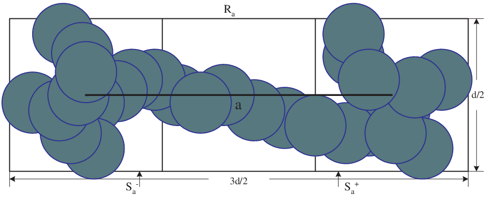
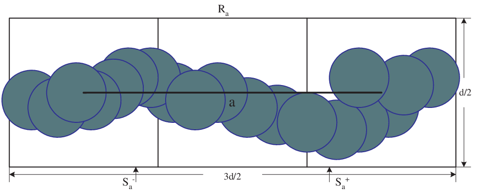
For edge $a$ in $\mathcal{L}$ , define event $A_{a}(d)$ as the set of outcomes for which the following condition holds: the rectangle $R_{a}=[a_{x}d-\frac{d}{4},a_{x}d+\frac{5d}{4}]\times[a_{y}d-\frac{d}{4},a_{y}d+\frac{d}{4}]$ is crossed²² 2 Here, a rectangle $R=[x_{1},x_{2}]\times[y_{1},y_{2}]$ being crossed from left to right by a connected component in $G(\mathcal{H}_{\lambda},1)$ means that there exists a sequence of nodes $v_{1},v_{2},...,v_{m}\in G(\mathcal{H}_{\lambda},1)$ contained in $R$ , with $||\mathbf{x}_{v_{i}}-\mathbf{x}_{v_{i+1}}||\leq 1,i=1,...,m-1$ , and $0<x(v_{1})-x_{1}<1,0<x_{2}-x(v_{m})<1$ , where $x(v_{1})$ and $x(v_{m})$ are the $x$ -coordinates of nodes $v_{1}$ and $v_{m}$ , respectively. A rectangle being crossed from top to bottom is defined analogously. from left to right by a connected component in $G(\mathcal{H}_{\lambda},1)$ . If $A_{a}(d)$ occurs, we say that rectangle $R_{a}$ is a good rectangle, and edge $a$ is a good edge. Let

p_{g}(d)\triangleq\Pr(A_{a}(d)).

Define $A_{a}(d)$ similarly for all vertical edges by rotating the rectangle by $90^{\circ}$ . An example of a good rectangle and a good edge is illustrated in Figure 1-(a).

Further define event $B_{a}(d)$ for edge $a$ in $\mathcal{L}$ as the set of outcomes for which both of the following hold: (i) $A_{a}(d)$ occurs; (ii) the left square $S_{a}^{-}=[a_{x}d-\frac{d}{4},a_{x}d+\frac{d}{4}]\times[a_{y}d-\frac{d}{4},a_{y}d+\frac{d}{4}]$ and the right square $S_{a}^{+}=[a_{x}d+\frac{3d}{4},a_{x}d+\frac{5d}{4}]\times[a_{y}d-\frac{d}{4},a_{y}d+\frac{d}{4}]$ are both crossed from top to bottom by connected components in $G_{1}(\mathcal{H}_{\lambda},1)$ .

If $B_{a}(d)$ occurs, we say that rectangle $R_{a}$ is an open rectangle, and edge $a$ is an open edge. Let

p_{o}(d)\triangleq\Pr(B_{a}(d)).

Define $B_{a}(d)$ similarly for all vertical edges by rotating the rectangle by $90^{\circ}$ . Examples of an open rectangle and an open edge are illustrated in Figure 1-(b).

Suppose edges $b$ and $c$ are vertically adjacent to edge $a$ , then it is clear that if events $A_{a}(d)$ , $A_{b}(d)$ and $A_{c}(d)$ all occur, then event $B_{a}(d)$ occurs. Moreover, since events $A_{a}(d)$ , $A_{b}(d)$ and $A_{c}(d)$ are increasing events³³ 3 An event $A$ is called increasing if $I_{A}(G)\leq I_{A}(G^{\prime})$ whenever graph $G$ is a subgraph of $G^{\prime}$ , where $I_{A}$ is the indicator function of $A$ . An event $A$ is called decreasing if $A^{c}$ is increasing. For details, please see [3, 4, 5]., by the FKG inequality [3, 4, 5],

$\displaystyle p_{o}(d)$	$\displaystyle=$	$\displaystyle\Pr(B_{a}(d))$
	$\displaystyle\geq$	$\displaystyle\Pr(A_{a}(d)\cap A_{b}(d)\cap A_{c}(d))$
	$\displaystyle\geq$	$\displaystyle\Pr(A_{a}(d))\Pr(A_{b}(d))\Pr(A_{c}(d))$
	$\displaystyle=$	$\displaystyle(p_{g}(d))^{3}.$

According to Corollary 4.1 in [4], the probability $p_{g}(d)$ converges to 1 as $d\rightarrow\infty$ when $G(\mathcal{H}_{\lambda},1)$ is in the supercritical phase. In this case, $(p_{g}(d))^{3}$ converges to 1 as $d\rightarrow\infty$ as well. Hence, $p_{o}(d)$ converges to 1 as $d\rightarrow\infty$ when $G(\mathcal{H}_{\lambda},1)$ is in the supercritical phase.

Note that in our model, the events $\{B_{a}(d)\}$ are not independent in general. However, if two edges $a$ and $b$ are not adjacent, i.e., they do not share any common end vertices, then $B_{a}(d)$ and $B_{b}(d)$ are independent. Furthermore, when edges $a$ and $b$ are adjacent, $B_{a}(d)$ and $B_{b}(d)$ are increasing events and thus positively correlated ⁴⁴ 4 Positive correlation means $\Pr(B_{a}(d)|B_{b}(d))>\Pr(B_{a}(d))$ .. Consequently, our model is a 1-dependent bond percolation model. It is known that there exists $p^{\mbox{\small{bond}}}_{\mbox{\small{1-dep}}}<1$ such that any 1-dependent model with $p>p^{\mbox{\small{bond}}}_{\mbox{\small{1-dep}}}$ is percolated, where $p$ is the probability of an edge being open [21].

Now define

d_{0}\triangleq\inf\left\{d^{\prime}>1:p_{o}(d^{\prime})>\max\left\{\frac{8}{9},p^{\mbox{\small{bond}}}_{\mbox{\small{1-dep}}}\right\}\right\},

(19)

and choose the edge length of $\mathcal{L}$ to be $d>d_{0}$ . Then there is an infinite cluster consisting of open edges and their end vertices in $\mathcal{L}$ . Denote this infinite cluster by $\mathcal{C}(\mathcal{L})$ .

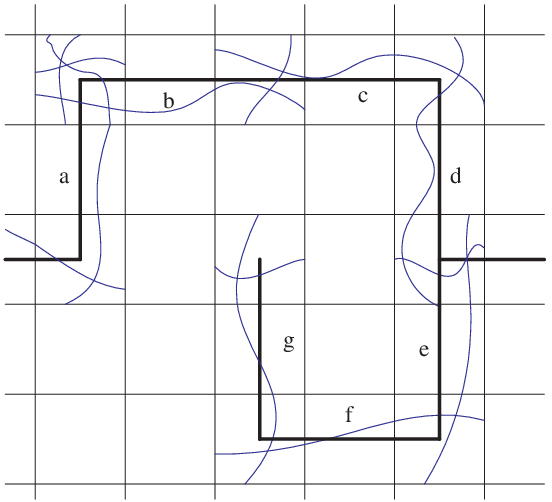
From Figure 2, it is easy to see that all the nodes along the crossings in $R_{a}$ and all the nodes along the crossings in $R_{b}$ for any $a,b\in\mathcal{C}(\mathcal{L})$ are connected. Since the infinite component of $G(\mathcal{H}_{\lambda},1)$ is unique, all the nodes along the crossings in $R_{a}$ for each $a\in\mathcal{C}(\mathcal{L})$ must belong to $\mathcal{C}(G(\mathcal{H}_{\lambda},1))$ .

By definition, no node of $G(\mathcal{H}_{\lambda},1)$ strictly inside $\mathcal{A}(\mathbf{0},r_{0})$ belongs to $\mathcal{C}(G(\mathcal{H}_{\lambda},1))$ . This implies that no edge of $\mathcal{L}$ strictly inside $\mathcal{A}(\mathbf{0},r_{0})$ belongs to $\mathcal{C}(\mathcal{L})$ . To see this, suppose edge $a_{i,j}$ of $\mathcal{L}$ is strictly inside $\mathcal{A}(\mathbf{0},r_{0})$ and belongs to $\mathcal{C}(\mathcal{L})$ . The nodes along the crossings in $R_{a_{i,j}}$ belong to $\mathcal{C}(G(\mathcal{H}_{\lambda},1))$ . As shown in Figure 3-(a), when $d>1$ and $r_{0}\gg 1$ , no matter what direction the edge $a_{i,j}$ has, there are some nodes along the crossings in $R_{a_{i,j}}$ (therefore belonging to $\mathcal{C}(G(\mathcal{H}_{\lambda},1))$ ) which are strictly inside $\mathcal{A}(\mathbf{0},r_{0})$ . These nodes then have strictly smaller distance to $\mathbf{0}$ than node $\mathbf{\tilde{X}}_{0}$ . This contradiction ensures that no edge of $\mathcal{L}$ strictly inside $\mathcal{A}(\mathbf{0},r_{0})$ belongs to $\mathcal{C}(\mathcal{L})$ .

Consider the dual lattice $\mathcal{L}^{\prime}$ of $\mathcal{L}$ . The construction of $\mathcal{L}^{\prime}$ is as follows: let each vertex of $\mathcal{L}^{\prime}$ be located at the center of a square of $\mathcal{L}$ . Let each edge of $\mathcal{L}^{\prime}$ be open if and only if it crosses an open edge of $\mathcal{L}$ , and closed otherwise. It is clear that each edge in $\mathcal{L}^{\prime}$ is open also with probability $p_{o}(d)$ . Let

q=1-p_{o}(d)<\frac{1}{9}.

Choose $2m$ edges in $\mathcal{L}^{\prime}$ . Since the states (open or closed) of any set of non-adjacent edges are independent, we can choose $m$ edges among the $2m$ edges such that their states are independent. As a result,

\Pr(\mbox{all the $2m$ edges are closed})\leq q^{m}.

Now a key observation is that if no edge of $\mathcal{L}$ strictly inside $\mathcal{A}(\mathbf{0},r_{0})$ belongs to $\mathcal{C}(\mathcal{L})$ , for which the event is denoted by $E_{\mathcal{L}}$ , then there must exist a closed circuit in $\mathcal{L}^{\prime}$ (a circuit consisting of closed edges) containing all edges of $\mathcal{L}$ strictly inside $\mathcal{A}(\mathbf{0},r_{0})$ , for which the event is denoted by $E_{\mathcal{L}^{\prime}}$ , and vice versa [3]. This is demonstrated in Figure 3-(b). Hence

\Pr(E_{\mathcal{L}})=1\Longleftrightarrow\Pr(E_{\mathcal{L}^{\prime}})=1.

Any closed circuit in $\mathcal{L}^{\prime}$ containing all edges of $\mathcal{L}$ strictly inside $\mathcal{A}(\mathbf{0},r_{0})$ has length greater than or equal to $2l$ , where $l\triangleq 2\lfloor\frac{r_{0}}{d}\rfloor$ . Thus we have

\Pr(E_{\mathcal{L}^{\prime}})=\sum_{m=l}^{\infty}\Pr(\exists\mathcal{O}_{c}(2m))\leq\sum_{m=l}^{\infty}\gamma(2m)q^{m},

where $\mathcal{O}_{c}(2m)$ is a closed circuit having length $2m$ in $\mathcal{L}^{\prime}$ containing all edges of $\mathcal{L}$ strictly inside $\mathcal{A}(\mathbf{0},r_{0})$ , and $\gamma(2m)$ is the number of such circuits. By Proposition 15 in Appendix B, we have $\gamma(2m)=\frac{4}{27}(m-1)3^{2m}$ so that

$\displaystyle\sum_{m=l}^{\infty}\gamma(2m)q^{m}$	$\displaystyle\leq$	$\displaystyle\sum_{m=l}^{\infty}\frac{4}{27}(m-1)(9q)^{m}$	(20)
	$\displaystyle=$	$\displaystyle\frac{4}{27}\left[\sum_{m=l}^{\infty}m(9q)^{m}-\sum_{m=l}^{\infty}(9q)^{m}\right]$
	$\displaystyle=$	$\displaystyle\frac{4[l-1-(l-2)9q]}{27(1-9q)^{2}}(9q)^{l}.$

Since $q<\frac{1}{9}$ , we have $\Pr(E_{\mathcal{L}^{\prime}})\rightarrow 0$ as $l=2\lfloor\frac{r_{0}}{d}\rfloor\rightarrow\infty$ . That is, as $r_{0}$ goes to infinity, with probability 1, there is some edge of $\mathcal{L}$ strictly inside $\mathcal{A}(\mathbf{0},r_{0})$ belonging to $\mathcal{C}(\mathcal{L})$ . Hence, with probability 1, there is some node of $G(\mathcal{H}_{\lambda},1)$ strictly inside $\mathcal{A}(\mathbf{0},r_{0})$ belonging to $\mathcal{C}(G(\mathcal{H}_{\lambda},1))$ . This contradiction implies that $r_{0}$ is finite with probability 1.∎

Let $r_{m}=||\tilde{\mathbf{X}}_{m}-(m,0)||$ , by Lemma 8 and stationarity, we have $r_{m}<\infty$ with probability 1, for any $m$ .

Lemma 9

Let $L(\mathbf{\tilde{X}}_{0},\mathbf{\tilde{X}}_{m})$ be the shortest path (in terms of the number of links) from $\mathbf{\tilde{X}}_{0}$ to $\mathbf{\tilde{X}}_{m}$ , and let $|L(\mathbf{\tilde{X}}_{0},\mathbf{\tilde{X}}_{m})|$ denote the number of links on such a path. If $||\mathbf{\tilde{X}}_{0}-\mathbf{\tilde{X}}_{m}||<\infty$ , then $|L(\mathbf{\tilde{X}}_{0},\mathbf{\tilde{X}}_{m})|<\infty$ , and $E[T_{0,m}^{L}]<\infty$ , where $T_{0,m}^{L}$ denotes the delay on path $L(\mathbf{\tilde{X}}_{0},\mathbf{\tilde{X}}_{m})$ .

Proof: We use the same mapping as the one for the proof of Lemma 8. For any given $\sqrt[4]{\frac{8}{9}}<\delta<1$ , define

d_{\delta}=\max\{\inf\{d^{\prime}:p_{g}(d^{\prime})\geq\delta\},||\mathbf{\tilde{X}}_{0}-\mathbf{\tilde{X}}_{m}||\}.

(21)

Then, for any $d>d_{\delta}$ , we have $p_{g}(d)\geq\delta$ .

Now, consider a fractal structure as shown in Figure 4: first a square $S(d_{\delta})$ is constructed with edge length $d_{\delta}$ centered at $\frac{\mathbf{\tilde{X}}_{0}+\mathbf{\tilde{X}}_{m}}{2}$ . Then, a second square $S(3d_{\delta})$ is constructed with edge length $3d_{\delta}$ also centered at $\frac{\mathbf{\tilde{X}}_{0}+\mathbf{\tilde{X}}_{m}}{2}$ . The construction proceeds in the same manner, i.e., at step $j$ , a square $S(3^{j-1}d_{\delta})$ is constructed with edge length $3^{j-1}d_{\delta}$ centered at $\frac{\mathbf{\tilde{X}}_{0}+\mathbf{\tilde{X}}_{m}}{2}$ . Thus, we have the initial square and a sequence of square annuli that do not overlap.

Denote the square annulus with inside edge length $3^{j-1}d_{\delta}$ ( $j\geq 2$ ) and outside edge length $3^{j}d_{\delta}$ by $D(3^{j}d_{\delta})$ . Let $A_{j}^{+}$ be the event that the upper horizontal rectangle of $D(3^{j}d_{\delta})$ — $[\frac{m}{2}-\frac{3^{j}}{2}d_{\delta},\frac{m}{2}+\frac{3^{j}}{2}d_{\delta}]\times[\frac{3^{j-1}}{2}d_{\delta},\frac{3^{j}}{2}d_{\delta}]$ is good, i.e., it is crossed by a connected component in $G(\mathcal{H}_{\lambda},1)$ from left to right. Since the length of the corresponding lattice edge of the upper horizontal rectangle of $D(3^{j}d_{\delta})$ is $2\cdot 3^{j-1}d_{\delta}>d_{\delta}$ , we have $\mbox{Pr}\{A_{j}^{+}\}\geq\delta$ . Similarly define $A_{j}^{-}$ , $B_{j}^{+}$ and $B_{j}^{-}$ to be the events that the lower, right and left rectangles are good, respectively. Then $\mbox{Pr}\{A_{j}^{-}\}\geq\delta$ , $\mbox{Pr}\{B_{j}^{+}\}\geq\delta$ and $\mbox{Pr}\{B_{j}^{-}\}\geq\delta,\forall j\geq 1$ .

Let $E_{j}$ be the event that there exists a circuit of connected nodes in $G(\mathcal{H}_{\lambda},1)$ within $D(3^{j}d_{\delta})$ . Once $A_{j}^{+},A_{j}^{-},B_{j}^{+}$ and $B_{j}^{-}$ all occur, $E_{j}$ must also occur. Although $A_{j}^{+},A_{j}^{-},B_{j}^{+}$ and $B_{j}^{-}$ are not independent, they are increasing events. By the FKG inequality, we have

$\displaystyle\Pr(E_{j})$	$\displaystyle\geq$	$\displaystyle\Pr(A_{j}^{+}\cap A_{j}^{-}\cap B_{j}^{+}\cap B_{j}^{-})$	(22)
	$\displaystyle\geq$	$\displaystyle\Pr(A_{j}^{+})\Pr(A_{j}^{-})\Pr(B_{j}^{+})\Pr(B_{j}^{-})$
	$\displaystyle\geq$	$\displaystyle\delta^{4}.$

When $E_{j}$ occurs, $\mathbf{\tilde{X}}_{0}$ and $\mathbf{\tilde{X}}_{m}$ are contained in $S(3^{j-1}d_{\delta})$ and there is a circuit of connected nodes in $G(\mathcal{H}_{\lambda},1)$ contained in the square annulus $D(3^{j}d_{\delta})$ . If the shortest path between $\mathbf{\tilde{X}}_{0}$ and $\mathbf{\tilde{X}}_{m}$ , $L(\mathbf{\tilde{X}}_{0},\mathbf{\tilde{X}}_{m})$ , were to go outside $S(3^{j}d_{\delta})$ , it would intersect the closed circuit contained by $D(3^{j}d_{\delta})$ and we could construct a shorter path from $\mathbf{\tilde{X}}_{0}$ to $\mathbf{\tilde{X}}_{m}$ . This implies that $L(\mathbf{\tilde{X}}_{0},\mathbf{\tilde{X}}_{m})$ must be contained in $S(3^{j}d_{\delta})$ .

Suppose $u$ , $v$ and $w$ are three consecutive nodes along $L(\mathbf{\tilde{X}}_{0},\mathbf{\tilde{X}}_{m})$ . Then $||\mathbf{X}_{u}-\mathbf{X}_{w}||>1$ , since otherwise $v$ would not belong to the shortest path. Hence, if we draw circles with radius $\frac{1}{2}$ , centered at $\mathbf{X}_{u}$ and $\mathbf{X}_{w}$ , respectively, then the two circles do not overlap. Consequently, if the length of $L(\mathbf{\tilde{X}}_{0},\mathbf{\tilde{X}}_{m})$ is $|L|\triangleq|L(\mathbf{\tilde{X}}_{0},\mathbf{\tilde{X}}_{m})|$ , then we must be able to draw at least $\lceil\frac{|L|}{2}\rceil$ circles with radius $\frac{1}{2}$ centered at alternating nodes along $L(\mathbf{\tilde{X}}_{0},\mathbf{\tilde{X}}_{m})$ . All of these circles are contained in the square with edge length $3^{j}d_{\delta}+1$ . Such a square contains at most $\lceil(3^{j}d_{\delta}+1)^{2}/[\pi(\frac{1}{2})^{2}]\rceil$ non-overlapping circles with radius $\frac{1}{2}$ . Therefore, $|L|\leq 2\lceil 4(3^{j}d_{\delta}+1)^{2}/\pi\rceil<\infty$ .

Now if $|L|>2\lceil 4(3^{j}d_{\delta}+1)^{2}/\pi\rceil$ , then $|L|>2\lceil 4(3^{i}d_{\delta}+1)^{2}/\pi\rceil$ for all $i=1,2,...,j$ . By the above argument, none of the events $E_{1},E_{2},...E_{j}$ can occur. Thus

\Pr\left(|L|>2\left\lceil\frac{4}{\pi}(3^{j}d_{\delta}+1)^{2}\right\rceil\right)\leq\prod_{i=1}^{j}\Pr(E_{i}^{c})\leq(1-\delta^{4})^{j}.

Let $M=2\left\lceil\frac{4}{\pi}(3d_{\delta}+1)^{2}\right\rceil$ , then we have

$\displaystyle E[\|L\|]$	$\displaystyle=$	$\displaystyle\sum_{k=0}^{\infty}\Pr(\|L\|>k)$	(23)
	$\displaystyle=$	$\displaystyle\sum_{k=0}^{M}\Pr(\|L\|>k)+\sum_{k=M+1}^{\infty}\Pr(\|L\|>k)$
	$\displaystyle\leq$	$\displaystyle M+\sum_{j=1}^{\infty}\left\lceil\frac{4}{\pi}(3^{j+1}d_{\delta}+1)^{2}\right\rceil\Pr\left(\|L\|>\left\lceil\frac{4}{\pi}(3^{j}d_{\delta}+1)^{2}\right\rceil\right)$
	$\displaystyle\leq$	$\displaystyle M+\sum_{j=1}^{\infty}\left(\frac{4}{\pi}(3^{j+1}d_{\delta}+1)^{2}+1\right)(1-\delta^{4})^{j}$
	$\displaystyle=$	$\displaystyle M+\sum_{j=1}^{\infty}\left(\frac{4}{\pi}(9\cdot 9^{j}d^{2}_{\delta}+6\cdot 3^{j}d_{\delta}+1)+1\right)(1-\delta^{4})^{j}$
	$\displaystyle=$	$\displaystyle M+\frac{36d^{2}_{\delta}}{\pi}\sum_{j=1}^{\infty}9^{j}(1-\delta^{4})^{j}+\frac{24d_{\delta}}{\pi}\sum_{j=1}^{\infty}3^{j}(1-\delta^{4})^{j}+\left(\frac{4}{\pi}+1\right)\sum_{j=1}^{\infty}(1-\delta^{4})^{j}.$

When $\delta>\sqrt[4]{\frac{8}{9}}$ , we have $(1-\delta^{4})^{j}<9^{-j}$ . Thus, $E[|L|]<\infty$ .

Let $\Lambda_{W(d,t)}\triangleq\sup_{0<d\leq 1}\{\eta_{0}(d)E[Y_{k}(d)]\}<\infty$ , then

E[T_{0,m}^{L}||L|]=\sum_{i=1}^{|L|}\eta_{0}^{(i)}(d)E[Y_{k}^{(i)}(d)]\leq|L|\Lambda_{W(d,t)},

(24)

where $\eta_{0}^{(i)}(d)$ and $E[Y_{k}^{(i)}(d)]$ are the stationary probability of the inactive state, and the expected inactive period of the $i$ -th link with length $d$ on $L(\mathbf{\tilde{X}}_{0},\mathbf{\tilde{X}}_{m})$ , respectively. Hence

E[T_{0,m}^{L}]=E[E[T_{0,m}^{L}||L|]]\leq E[|L|]\Lambda_{W(d,t)}<\infty.

(25)

∎

To show property (v), we show $\{T_{(m-1)j,mj},m\geq 1\}$ is strong mixing.⁵⁵ 5 A measure preserving transformation $H$ on $(\Omega,\mathcal{F},P)$ is called strong mixing if for all measurable sets $A$ and $B$ , $\lim_{m\rightarrow\infty}|P(A\cap H^{-m}B)-P(A)P(B)|=0$ . A sequence $\{X_{n},n\geq 0\}$ is called strong mixing if the shift on sequence space is strong (weak) mixing. Every strong mixing system is ergodic [22].

Lemma 10

The sequence $\{T_{(m-1)k,mk},m\geq 1\}$ is strong mixing, so that it is ergodic.

Proof: From the proof of Lemma 8, we have $\Pr(E_{j})\geq\delta^{4}$ for all $j=1,2,...$ . Summing over $j$ yields

\sum_{j=1}^{\infty}\Pr(E_{j})\geq\sum_{j=1}^{\infty}\delta^{4}=\infty.

(26)

Since ${E_{j}}$ are independent events, by the Borel-Cantelli Lemma, with probability 1, there exists $j^{\prime}<\infty$ such that $E_{j^{\prime}}$ occurs.

We now construct squares $A_{1}$ and $A_{2}$ centered at $\frac{\mathbf{\tilde{X}}_{(m-1)j}+\mathbf{\tilde{X}}_{mj}}{2}$ and $\frac{\mathbf{\tilde{X}}_{(m+k-1)j}+\mathbf{\tilde{X}}_{(m+k)j}}{2}$ with edge length $3^{j^{\prime}}d_{\delta}$ and $3^{j^{\prime\prime}}d_{\delta}$ respectively, such that the path with the smallest delay from $\mathbf{\tilde{X}}_{(m-1)j}$ to $\mathbf{\tilde{X}}_{mj}$ , and the path with the smallest delay from $\mathbf{\tilde{X}}_{(m+k-1)j}$ to $\mathbf{\tilde{X}}_{(m+k)j}$ are contained in $A_{1}$ and $A_{2}$ , respectively. Let $E$ be the event that $j^{\prime}<\infty$ and $j^{\prime\prime}<\infty$ . Then $\Pr(E)=1$ .

When finite $j^{\prime}$ and $j^{\prime\prime}$ exist, due to stationarity, $j^{\prime}$ and $j^{\prime\prime}$ are independent of $k$ . Hence, as $k\rightarrow\infty$ , $A_{1}$ and $A_{2}$ become non-overlapping so that the paths inside $A_{1}$ and $A_{2}$ do not share any common nodes of $G(\mathcal{H}_{\lambda},1)$ . Hence $T_{(m-1)j,mj}$ and $T_{(m+k-1)j,(m+k)j}$ are independent of each other as $k\rightarrow\infty$ . This is illustrated in Figure 5.

Therefore

	$\displaystyle\lim_{k\rightarrow\infty}\Pr(\{T_{(m-1)j,mj}<t\}\cap\{T_{(m+k-1)j,(m+k)j}<t^{\prime}\})$	(27)
$\displaystyle=$	$\displaystyle\lim_{k\rightarrow\infty}\Pr(\{T_{(m-1)j,mj}<t\}\cap\{T_{(m+k-1)j,(m+k)j}<t^{\prime}\}\|E)\Pr(E)$
	$\displaystyle+\lim_{k\rightarrow\infty}\Pr(\{T_{(m-1)j,mj}<t\}\cap\{T_{(m+k-1)j,(m+k)j}<t^{\prime}\}\|E^{c})\Pr(E^{c})$
$\displaystyle=$	$\displaystyle\Pr(T_{(m-1)j,mj}<t\|E)\Pr(T_{(m-1)j,mj}<t^{\prime}\|E)$
$\displaystyle=$	$\displaystyle\Pr(T_{(m-1)j,mj}<t)\Pr(T_{(m-1)j,mj}<t^{\prime}),$

This implies that sequence $\{T_{(m-1)k,mk},m\geq 1\}$ is strong mixing, so that it is ergodic.∎

Now, we present the proof for Lemma 6.

Proof of Lemma 6: Conditions (i)–(iii) of Theorem 7 have been verified. The validation of (iv) is provided by Lemma 9. Let $L(\mathbf{\tilde{X}}_{0},\mathbf{\tilde{X}}_{m})$ be the shortest path from $\mathbf{\tilde{X}}_{0}$ to $\mathbf{\tilde{X}}_{m}$ . Since $L(\mathbf{\tilde{X}}_{0},\mathbf{\tilde{X}}_{m})$ is a particular path, we have $T_{0,m}\leq T_{0,m}^{L}$ so that $E[T_{0,m}]\leq E[T_{0,m}^{L}]$ , where $T_{0,m}^{L}$ denotes the delay on path $L(\mathbf{\tilde{X}}_{0},\mathbf{\tilde{X}}_{m})$ . By Lemma 9, we have $E[T_{0,m}^{L}]<\infty$ and therefore $E[T_{0,m}]<\infty$ . Furthermore, due to Lemma 10, $\{T_{(m-1)k,mk},m\geq 1\}$ is ergodic, thus the results (a) and (b) of Theorem 7 hold.∎

Remark: Using the proof for condition (iv) of Theorem 7, we can show that for any two nodes $u$ and $v$ in the infinite component of $G(\mathcal{H}_{\lambda},1)$ which are within finite Euclidean distance of each other, i.e., $u,v\in\mathcal{C}(G(\mathcal{H}_{\lambda},1))$ with $d(u,v)<\infty$ , $E[T(u,v)]<\infty$ .

The following lemma asserts that the constant $\gamma$ defined in (18) assumes different values according to whether $G(\mathcal{H}_{\lambda},1,W(d,t))$ is in the subcritical phrase or the supercritical phase.

Lemma 11

Let $\gamma$ be defined as (18). (i) If $G(\mathcal{H}_{\lambda},1,W(d,t))$ is in the subcritical phase, i.e., $\lambda<\lambda_{c}(\eta_{1}(d))$ , then $\gamma<\infty$ , and $\gamma>0$ with probability 1. (ii) If $G(\mathcal{H}_{\lambda},1,W(d,t))$ is in the supercritical phase, i.e., $\lambda>\lambda_{c}(\eta_{1}(d))$ , then $\gamma=0$ with probability 1.

Proof: To show (i), note that $\gamma<\infty$ follows directly from

\gamma=\inf_{m\geq 1}\frac{E[T_{0,m}]}{m}\leq E[T_{0,1}]<\infty,

(28)

where the last inequality is shown above in the proof for Lemma 6.

To see why $\gamma$ is positive with probability 1, suppose the node at $\mathbf{\tilde{X}}_{0}$ disseminates a message at time $t=t_{0}$ and consider $G(\mathcal{H}_{\lambda},1,W(d,t_{0}))$ . Choose $K$ large enough such that $c_{1}e^{-c_{2}K}<\frac{1}{2}$ , where $c_{1}$ and $c_{2}$ are the constants given in Proposition 3. Let $q=\lfloor\frac{m}{2(K+1)}\rfloor$ . When $m>2(K+1)$ , $q\geq 1$ .

Let $S_{h}=\{(x,y)\in\mathbb{R}^{2}:K+(h-1)(K+1)\leq x-x(\mathbf{\tilde{X}}_{0})<h(K+1)\}$ for $h=1,2,...$ , where $x(v)$ is the $x$ -coordinate of node $v$ . Since $\mathbf{\tilde{X}}_{0}$ and $\mathbf{\tilde{X}}_{m}$ are both in $\mathcal{C}(G(\mathcal{H}_{\lambda},1))$ , there exists at least one path from $\mathbf{\tilde{X}}_{0}$ to $\mathbf{\tilde{X}}_{m}$ . Moreover, since each strip $S_{h}$ has width 1, at least one node of $\mathcal{C}(G(\mathcal{H}_{\lambda},1))$ lies inside each $S_{h}$ .

Let $\{\mathbf{X}^{(1)}_{l},l=1,2,...\}$ be the nodes of $\mathcal{C}(G(\mathcal{H}_{\lambda},1))$ which lie inside $S_{1}$ . Since $G(\mathcal{H}_{\lambda},1,W(d,t_{0}))$ is in the subcritical phase, by Proposition 3, the probability that there exists a path consisting of only active links from $\mathbf{\tilde{X}}_{0}$ to any $\mathbf{X}^{(1)}_{l}$ , $l=1,2,...$ , is less than or equal to $c_{1}e^{-c_{2}K}<\frac{1}{2}$ . In other words, with probability strictly greater than $\frac{1}{2}$ , there exists at least one inactive link at time $t=t_{0}$ on any path from $\mathbf{\tilde{X}}_{0}$ to $\mathbf{X}^{(1)}_{l}$ , $l=1,2,...$ . Let $T^{(1)}=\inf_{l}\{T(\mathbf{\tilde{X}}_{0},\mathbf{X}^{(1)}_{l})\}$ . Let $\Gamma_{W(d,t)}\triangleq\inf_{0<d\leq 1}\left\{\eta_{0}(d)E[Y_{k}(d)]\right\}>0$ , then $E[T^{(1)}]>\frac{1}{2}\Gamma_{W(d,t)}>0$ .

Let $\{\mathbf{X}^{(h+1)}_{l^{\prime}},l^{\prime}=1,2,...\}$ be the nodes of $\mathcal{C}(G(\mathcal{H}_{\lambda},1))$ which lie inside $S_{h+1}$ , for $h\geq 1$ . By the same argument as above, the probability that there exists a path consisting of only active links from any node in $S_{h}$ to any node in $S_{h+1}$ is less than or equal to $c_{1}e^{-c_{2}K}<\frac{1}{2}$ . In other words, with probability strictly greater than $\frac{1}{2}$ , there exists at least one inactive link on any path from any node in $S_{h}$ to any node in $S_{h+1}$ . Let $T^{(h+1)}=\inf_{l,l^{\prime}}\{T(\mathbf{X}^{(h)}_{l},\mathbf{X}^{(h+1)}_{l^{\prime}})\}$ . Then $E[T^{(h+1)}]>\frac{1}{2}\Gamma_{W(d,t)}>0$ . The path segments are illustrated in Figure 6.

Since $||\mathbf{\tilde{X}}_{0}-\mathbf{\tilde{X}}_{m}||\geq m-r_{0}-r_{m}$ , when $\frac{m}{2}>r_{0}+r_{m}$ , any path from $\mathbf{\tilde{X}}_{0}$ to $\mathbf{\tilde{X}}_{m}$ has at least $\lfloor\frac{m}{2(K+1)}\rfloor=q$ segments and the delay on each segment is strictly greater than $\frac{1}{2}\Gamma_{W(d,t)}>0$ . Hence, $E[T_{0,m}]>\frac{1}{2}q\Gamma_{W(d,t)}$ when $\frac{m}{2}>r_{0}+r_{m}$ . Since both $r_{0}$ and $r_{m}$ are finite with probability 1, $\frac{m}{2}>r_{0}+r_{m}$ holds with probability 1 as $m\rightarrow\infty$ .

Since $K$ is finite and $\Gamma_{W(d,t)}$ is positive and independent of $m$ , we have

$\displaystyle\gamma$	$\displaystyle=$	$\displaystyle\lim_{m\rightarrow\infty}\frac{E[T_{0,m}]}{m}$	(29)
	$\displaystyle>$	$\displaystyle\lim_{m\rightarrow\infty}\frac{q}{m}\frac{1}{2}\Gamma_{W(d,t)}$
	$\displaystyle>$	$\displaystyle\lim_{m\rightarrow\infty}\left(\frac{1}{2(K+1)}-\frac{1}{m}\right)\frac{1}{2}\Gamma_{W(d,t)}$
	$\displaystyle>$	$\displaystyle 0$

with probability 1, where we used the fact that $q>\frac{m}{2(K+1)}-1$ .

For (ii), suppose $G(\mathcal{H}_{\lambda},1,W(d,t))$ is in the supercritical phase. To simplify notation, let $\mathcal{C}(t)$ be the infinite component of $G(\mathcal{H}_{\lambda},1,W(d,t))$ . Let $t^{\prime}$ be the first time when some node in $\mathcal{C}(t^{\prime})$ receives $\mathbf{\tilde{X}}_{0}$ ’s message, and let

w_{1}\triangleq\argmin_{i\in\mathcal{C}(t^{\prime})}d(\mathbf{X}_{i},\mathbf{\tilde{X}}_{0}),\quad\mbox{and}\quad w_{2}\triangleq\argmin_{i\in\mathcal{C}(t^{\prime})}d(\mathbf{X}_{i},\mathbf{\tilde{X}}_{m}).

That is, $w_{1}$ and $w_{2}$ are the nodes in the infinite component of $G(\mathcal{H}_{\lambda},1,W(d,t^{\prime}))$ with the smallest Euclidean distances to nodes $\mathbf{\tilde{X}}_{0}$ and $\mathbf{\tilde{X}}_{m}$ , respectively. If node $\mathbf{\tilde{X}}_{0}$ is in $\mathcal{C}(t_{0})$ , then $t^{\prime}=t_{0}$ and $w_{1}=\mathbf{\tilde{X}}_{0}$ . If at time $t^{\prime}$ , node $v$ is in $\mathcal{C}(t^{\prime})$ , then $w_{2}=\mathbf{\tilde{X}}_{m}$ .

Since both $w_{1}$ and $w_{2}$ belong to $\mathcal{C}(t^{\prime})$ , $T(w_{1},w_{2})=0$ . The distances $d(\mathbf{\tilde{X}}_{0},\mathbf{X}_{w_{1}})$ and $d(\mathbf{X}_{w_{2}},\mathbf{\tilde{X}}_{m})$ are finite with probability 1 by Lemma 16 in Appendix C. Clearly, $d(\mathbf{\tilde{X}}_{0},\mathbf{X}_{w_{1}})$ is independent of $m$ . By stationarity, $d(\mathbf{X}_{w_{2}},\mathbf{\tilde{X}}_{m})$ is also independent of $m$ . Hence, by the proof of Lemma 6, $E[T(\mathbf{\tilde{X}}_{0},\mathbf{X}_{w_{1}})]<\infty$ , $E[T(\mathbf{X}_{w_{2}},\mathbf{\tilde{X}}_{m})]<\infty$ with probability 1 for any $m$ , and $E[T(\mathbf{\tilde{X}}_{0},\mathbf{X}_{w_{1}})]$ and $E[T(\mathbf{X}_{w_{2}},\mathbf{\tilde{X}}_{m})]$ are independent of $m$ . Moreover,

	$\displaystyle 0\leq\frac{T_{0,m}}{m}$	$\displaystyle\leq$	$\displaystyle\frac{T(\mathbf{\tilde{X}}_{0},\mathbf{X}_{w_{1}})+T(w_{1},w_{2})+T(\mathbf{X}_{w_{2}},\mathbf{\tilde{X}}_{m})}{m}$		(30)
		$\displaystyle=$	$\displaystyle\frac{T(\mathbf{\tilde{X}}_{0},\mathbf{X}_{w_{1}})+T(\mathbf{X}_{w_{2}},\mathbf{\tilde{X}}_{m})}{m}.$		(30)

Hence $\gamma=\lim_{m\rightarrow\infty}\frac{E[T_{0,m}]}{m}=0$ with probability 1. ∎

We are now ready to prove Theorem 5.

Proof of Theorem 5: Assume node $u$ disseminates a message at time $t=t_{0}$ . Take $\mathbf{X}_{u}$ as the origin, and the line $\mathbf{X}_{u}\mathbf{X}_{v}$ as the $x$ -axis. By definition $u,v\in\mathcal{C}(G(\mathcal{H}_{\lambda},1))$ . Since node $u$ is the origin, $\mathbf{X}_{u}=\tilde{\mathbf{X}}_{0}$ . Let $m$ be the closest integer to $x(v)$ —the $x$ -axis coordinate of node $\mathbf{X}_{v}$ . Now $T_{0,m}=T(\mathbf{X}_{u},\mathbf{\tilde{X}}_{m})$ . If $\mathbf{X}_{v}=\mathbf{\tilde{X}}_{m}$ , $T(u,v)=T_{0,m}$ .

Note that $m-1<d(u,v)<m+1$ , Thus, for any $m>1$ , we have

\frac{T_{0,m}}{m+1}<\frac{T(u,v)}{d(u,v)}<\frac{T_{0,m}}{m-1}.

(31)

On the other hand, if $\mathbf{X}_{v}\neq\mathbf{\tilde{X}}_{m}$ , then $\mathbf{\tilde{X}}_{m}$ must be adjacent to $\mathbf{X}_{v}$ . This is because $||(m,0)-\mathbf{X}_{v}||\leq\frac{1}{2}$ ( $m$ is the closest integer to $x(v)$ ) and $||(m,0)-\mathbf{\tilde{X}}_{m}||\leq\frac{1}{2}$ ( $\mathbf{\tilde{X}}_{m}$ is the closest node to $(m,0)$ ). Consequently, $T_{0,m}-T(\mathbf{\tilde{X}}_{m},\mathbf{X}_{v})\leq T(u,v)\leq T_{0,m}+T(\mathbf{\tilde{X}}_{m},\mathbf{X}_{v})$ . Thus, for any $m>1$ , we have

\frac{T_{0,m}-T(\mathbf{\tilde{X}}_{m},\mathbf{X}_{v})}{m+1}<\frac{T(u,v)}{d(u,v)}<\frac{T_{0,m}+T(\mathbf{\tilde{X}}_{m},\mathbf{X}_{v})}{m-1}.

(32)

Since $\mathbf{\tilde{X}}_{m}$ is adjacent to $\mathbf{X}_{v}$ , $T(\mathbf{\tilde{X}}_{m},\mathbf{X}_{v})<\infty$ with probability 1. Therefore, in both cases, by Lemma 6 and a typical $\epsilon$ - $\delta$ argument (see Appendix D), we have for any $\epsilon>0,\delta>0$ , there exists $d_{0}<\infty$ , such that if $d(u,v)>d_{0}$ , then

\Pr\left(\left|\frac{T(u,v)}{d(u,v)}-\gamma\right|<\epsilon\right)>1-\delta.

(33)

When $G(\mathcal{H}_{\lambda},1)$ is in the subcritical phase, by Lemma 11, we have $0<\gamma<\infty$ with probability 1.

On the other hand, when $G(\mathcal{H}_{\lambda},1)$ is in the supercritical phase, by Lemma 11, we have $\gamma=0$ with probability 1. Then, by a typical $\epsilon$ - $\delta$ argument (see Appendix E), we have for any $\epsilon>0,\delta>0$ , there exists $d_{0}<\infty$ , such that if $d(u,v)>d_{0}$ then

\Pr\left(\frac{T(u,v)}{d(u,v)}<\epsilon\right)>1-\delta.

∎

IV-C Effects of Propagation Delay

Up to this point, we have ignored propagation delays. We now take this type of delay into account. Suppose the propagation delay is $0<\tau<\infty$ for any link, independent of the link length. We assume the following mechanism is used for a transmission from node $i$ to node $j$ : (i) a packet is successfully received by node $j$ if the length of the active period on link $(i,j)$ , during which the packet is being transmitted, is greater than or equal to $\tau$ ; (ii) node $i$ retransmits a packet to node $j$ until the packet is successfully received by $j$ .

Note that due to the Markovian nature of the link state processes $\{W_{ij}(d_{ij},t)\}$ , at the instant when a packet arrives at node $i$ , the residual active time for link $(i,j)$ has the same distribution as $Z(d_{ij})$ . Thus without loss of generality, we assume that node $i$ initiates transmission on link $(i,j)$ at time $0$ . If link $(i,j)$ is on at time 0 with $Z_{1}(d)\geq\tau$ , then the transmission delay $T^{\tau}_{ij}(d)$ on $(i,j)$ is $\tau$ . However, if link $(i,j)$ is on at time 0 with $Z_{1}(d)<\tau$ , or if $(i,j)$ is off at time $t=0$ , then the delay on $(i,j)$ is less straightforward to calculate. In this case, we need to capture the behavior of retransmissions. Let

K(d)=\argmin_{k\geq 1}\{Z_{k}(d)\geq\tau\}.

(34)

Then, $K(d)$ is a stopping time for the sequence $\{Z_{k}(d),k\geq 1\}$ . Now we have

\left\{\begin{array}[]{lll}T^{\tau}_{ij}=\displaystyle\sum_{i=1}^{K-1}(Y_{i}+Z_{i})+Y_{K}+\tau,&W(d,0)=0,\\ T^{\tau}_{ij}=\displaystyle\sum_{i=1}^{K-1}(Y_{i}+Z_{i})+\tau,&W(d,0)=1,\end{array}\right.

(35)

where we abbreviate $T^{\tau}_{ij}(d)$ , $K(d)$ , $Y_{i}(d)$ and $Z_{i}(d)$ as $T^{\tau}_{ij}$ , $K$ , $Y_{i}$ and $Z_{i}$ , respectively.

Let

T^{\tau}(u,v)=T^{\tau}(\mathbf{X}_{u},\mathbf{X}_{v})\triangleq\inf_{l(u,v)\in\mathcal{L}(u,v)}\left\{\sum_{(i,j)\in l(u,v)}T^{\tau}_{ij}(d_{ij})\right\},

(36)

where $T^{\tau}_{ij}(d_{ij})$ is given by (35). Then, $T^{\tau}(u,v)$ is the message delay on the path from $u$ to $v$ with the smallest delay, including propagation delays.

Corollary 12

Given $G(\mathcal{H}_{\lambda},1,W(d,t))$ with $\lambda>\lambda_{c}$ and propagation delay $0<\tau<\infty$ , there exists a constant $\gamma(\tau)<\infty$ with $\gamma(\tau)\geq\tau$ (with probability 1), such that for any $u,v\in\mathcal{C}(G(\mathcal{H}_{\lambda},1))$ , and any $\epsilon>0,\delta>0$ , there exists $d_{0}<\infty$ such that for any $u,v$ with $d(u,v)>d_{0}$ ,

\Pr\left(\left|\frac{T^{\tau}(u,v)}{d(u,v)}-\gamma(\tau)\right|<\epsilon\right)>1-\delta.

(37)

Moreover, when $G(\mathcal{H}_{\lambda},1,W(d,t))$ is in the subcritical phase, as $\tau\rightarrow 0$ , $\gamma(\tau)\rightarrow\gamma$ with probability 1, where $\gamma$ is defined in Theorem 5. When $G(\mathcal{H}_{\lambda},1,W(d,t))$ is in the supercritical phase, as $\tau\rightarrow 0$ , $\gamma(\tau)\rightarrow 0$ with probability 1.

To prove this corollary, we need the following two lemmas.

Lemma 13

Given any $0<\tau<\infty$ , for all $0<d\leq 1$ , the expected delay on each link $(i,j)$ is positive and finite, i.e.,

0<E[T^{\tau}_{ij}]<\infty.

(38)

Proof: By (35), we have

$\displaystyle E[T^{\tau}_{ij}]$	$\displaystyle=$	$\displaystyle E[E[T^{\tau}_{ij}\|W(d,0)]]$	(39)
	$\displaystyle=$	$\displaystyle\eta_{0}E[T^{\tau}_{ij}\|W(d,0)=0]+\eta_{1}E[T^{\tau}_{ij}\|W(d,0)=1]$
	$\displaystyle=$	$\displaystyle\eta_{0}E\left[\sum_{i=1}^{K-1}(Y_{i}+Z_{i})+Y_{K}+\tau\|Z_{i}<\tau,i=1,...,K-1\right]$
		$\displaystyle+\eta_{1}E\left[\sum_{i=1}^{K-1}(Y_{i}+Z_{i})+\tau\|Z_{i}<\tau,i=1,...,K-1\right]$
	$\displaystyle=$	$\displaystyle\tau+\eta_{0}E[Y_{K}]+E\left[\sum_{i=1}^{K-1}(Y_{i}+Z_{i})\|Z_{i}<\tau,i=1,...,K-1\right]$
	$\displaystyle<$	$\displaystyle E[K]\tau+\eta_{0}E[Y_{K}]+(E[K]-1)E[Y_{i}],$

where in the last equality, we used the fact that $Y_{i}$ and $Z_{i}$ are i.i.d. and $Z_{i}<\tau$ for $i=1,2,...K-1$ , as well as Wald’s Equality for stopping time $K$ .

Since $0<\tau<\infty$ , $0<\eta_{0}<1$ , and $0<E[Y_{i}]<\infty$ , in order to show $0<E[T^{\tau}_{ij}]<\infty$ , it suffices to show $1\leq E[K]<\infty$ . By definition, $K\geq 1$ so that $E[K]\geq 1$ . Thus, we need only to show $E[K]<\infty$ . For any $k\geq 1$ , $\Pr(K=k)=\Pr(Z_{1}<\tau,...,Z_{k-1}<\tau,Z_{k}\geq\tau)=F_{Z}(\tau)^{k-1}(1-F_{Z}(\tau))$ , where $F_{Z}(\cdot)=\Pr(Z_{i}\leq\tau)$ . Then

E[K]=\sum_{k=1}^{\infty}kF_{Z}(\tau)^{k-1}(1-F_{Z}(\tau))=\frac{1}{1-F_{Z}(\tau)}.

(40)

Therefore, we have $E[K]<\infty$ . ∎

Lemma 14

Given $G(\mathcal{H}_{\lambda},1,W(d,t))$ with $\lambda>\lambda_{c}$ and no propagation delay, let $L_{0,m}$ be the path from $\mathbf{\tilde{X}_{0}}$ to $\mathbf{\tilde{X}_{m}}$ that attains $T_{0,m}$ and has the smallest number of links (in case there exist multiple paths attaining $T_{0,m}$ ). Then $|L_{0,m}|<\infty$ with probability 1 for each $m$ , where $|L_{0,m}|$ is the number of links along $L_{0,m}$ .

Proof: By the proof of Lemma 9, we have $E[T_{0,m}]<\infty$ . We can express $E[T_{0,m}]$ as

E[T_{0,m}]=E[E[T_{0,m}||L_{0,m}|]],

where

E[T_{0,m}||L_{0,m}|]=\sum_{i=1}^{|L_{0,m}|}\eta_{0}^{(i)}(d)E[Y_{k}^{(i)}(d)]\geq|L_{0,m}|\Gamma_{W(d,t)},

where $\eta_{0}^{(i)}(d)$ and $E[Y_{k}^{(i)}(d)]$ are the stationary probability of the inactive state, and the expected inactive period of the $i$ -th link with length $d$ on $L_{0,m}$ respectively, and $\Gamma_{W(d,t)}=\inf_{0<d\leq 1}\{\eta_{0}(d)E[Y_{k}(d)]\}>0$ . Thus, we have

E[|L_{0,m}|]\Gamma_{W(d,t)}<\infty.

This implies $E[|L_{0,m}|]<\infty$ , which further implies $|L_{0,m}|<\infty$ with probability 1. ∎

Proof of Corollary 12: Let $T^{\tau}_{l,m}=T^{\tau}(\mathbf{\tilde{X}}_{l},\mathbf{\tilde{X}}_{m})$ , for $||\mathbf{\tilde{X}}_{l}-\mathbf{\tilde{X}}_{m}||<\infty$ , $0\leq l\leq m$ , where $\mathbf{\tilde{X}}_{i}$ is defined as in (16).

Clearly, the relationship $T^{\tau}_{0,m}\leq T^{\tau}_{0,l}+T^{\tau}_{l,m}$ still holds for any $0\leq l\leq m$ . Hence, condition (i) of Theorem 7 holds. Since the propagation delay does not affect the stationarity of the geometric structure of the network, conditions (ii) and (iii) of Theorem 7 also hold.

By the same argument as that in the proof of Lemma 9, we have $E[|L|]<\infty$ , where $|L|\triangleq|L(\mathbf{\tilde{X}}_{0},\mathbf{\tilde{X}}_{m})|$ and $L(\mathbf{\tilde{X}}_{0},\mathbf{\tilde{X}}_{m})$ is the shortest path from $\mathbf{\tilde{X}}_{0}$ to $\mathbf{\tilde{X}}_{m}$ . Let $T^{\tau,L}_{0,m}$ be the delay on this path. Then,

E[T^{\tau,L}_{0,m}||L|]=\sum_{i=1}^{|L|}E[T^{\tau}_{i}(d_{i})]\leq|L|\Lambda_{W^{\tau}(d,t)},

where $T^{\tau}_{i}(d_{i})$ is the delay on the $i$ -th link with length $d_{i}$ on the path $L(\mathbf{\tilde{X}}_{0},\mathbf{\tilde{X}}_{m})$ , as given by (35), and $\Lambda_{W^{\tau}(d,t)}\triangleq\sup_{0<d\leq 1}E[T^{\tau}_{i}(d_{i})]<\infty$ . By Lemma 13, we have $0<E[T^{\tau}_{i}(d_{i})]<\infty$ for all $0<d_{i}\leq 1$ , so that $\Lambda_{W^{\tau}(d,t)}<\infty$ . Hence

E[T^{\tau,L}_{0,m}]=E[E[T^{\tau,L}_{0,m}||L|]]\leq E[|L|]\Lambda_{W^{\tau}(d,t)}<\infty,

which implies $E[T^{\tau}_{0,m}]<\infty$ . This ensures that condition (iv) of Theorem 7 holds.

Furthermore, the propagation delay does not affect the strong mixing property of $\{T^{\tau}_{l,m},0\leq l\leq m\}$ . Therefore the result of Lemma 6 holds for $\{T^{\tau}_{l,m},0\leq l\leq m\}$ . Let $\gamma(\tau)\triangleq\lim_{m\rightarrow\infty}\frac{E[T^{\tau}_{0,m}]}{m}$ , then $\gamma(\tau)=\inf_{m\geq 1}\frac{E[T^{\tau}_{0,m}]}{m}$ , and

\lim_{m\rightarrow\infty}\frac{T^{\tau}_{0,m}}{m}=\gamma(\tau)\quad\mbox{with probability 1}.

(41)

Then applying the same proof for Theorem 5, we can show that for any $\epsilon>0,\delta>0$ , there exists $d_{0}<\infty$ , such that if $d(u,v)>d_{0}$ , then

\Pr\left(\left|\frac{T^{\tau}(u,v)}{d(u,v)}-\gamma(\tau)\right|<\epsilon\right)>1-\delta.

To see why $\gamma(\tau)<\infty$ and $\gamma(\tau)\geq\tau$ with probability 1, first note that

\gamma(\tau)=\inf_{m\geq 1}\frac{E[T^{\tau}_{0,m}]}{m}\leq E[T^{\tau}_{0,1}]<\infty.

(42)

Moreover, since the shortest path between nodes $\mathbf{\tilde{X}}_{0}$ and $\mathbf{\tilde{X}}_{m}$ has at least $\lfloor||\mathbf{\tilde{X}}_{0}-\mathbf{\tilde{X}}_{m}||\rfloor\geq\lfloor m-r_{0}-r_{m}\rfloor$ links, $T^{\tau}_{0,m}\geq\tau\lfloor m-r_{0}-r_{m}\rfloor$ . Since $r_{0}$ and $r_{m}$ are both finite with probability 1 and independent of $m$ , we have $\gamma(\tau)\geq\tau$ with probability 1.

In the following, we show that as $\tau\rightarrow 0$ , $\gamma(\tau)\rightarrow\gamma$ with probability 1 when $G(\mathcal{H}_{\lambda},1)$ is in the subcritical phase, and $\gamma(\tau)\rightarrow 0$ with probability 1 when $G(\mathcal{H}_{\lambda},1)$ is in the supercritical phase. Observe that

T_{0,m}\leq T^{\tau}_{0,m}\leq\sum_{i=1}^{|L_{0,m}|}T^{\tau}_{i}(d_{i}),

where $L_{0,m}$ is defined in Lemma 14, and $T^{\tau}_{i}(d_{i})$ is the delay on the $i$ -th link with length $d_{i}$ along $L_{0,m}$ , as given by (35). From Lemma 14, we have $|L_{0,m}|<\infty$ with probability 1. Thus with probability 1,

E[T_{0,m}]\leq E[T^{\tau}_{0,m}]\leq\sum_{i=1}^{|L_{0,m}|}E[T^{\tau}_{i}(d_{i})].

By (39) and $E[T_{0,m}]=\sum_{i=1}^{|L_{0,m}|}\eta_{0}(d_{i})E[Y_{k}(d_{i})]$ we have

E[T_{0,m}]\leq E[T^{\tau}_{0,m}]\leq E[T_{0,m}]+|L_{0,m}|E[K]\tau+\sum_{i=1}^{|L_{0,m}|}(E[K]-1)E[Y_{k}(d_{i})],

(43)

with probability 1. From (40), we know that as $\tau\rightarrow 0$ , $E[K]\rightarrow 1$ . Therefore, as $\tau\rightarrow 0$ , we have $|L_{0,m}|E[K]\tau+\sum_{i=1}^{|L_{0,m}|}(E[K]-1)E[Y_{k}(d_{i})]\rightarrow 0$ with probability 1. This, combined with (43) implies $\lim_{\tau\rightarrow 0}E[T^{\tau}_{0,m}]=E[T_{0,m}]$ with probability 1. Therefore,

$\displaystyle\lim_{\tau\rightarrow 0}\gamma(\tau)$	$\displaystyle=$	$\displaystyle\lim_{\tau\rightarrow 0}\lim_{m\rightarrow\infty}\frac{E[T^{\tau}_{0,m}]}{m}$	(44)
	$\displaystyle=$	$\displaystyle\lim_{m\rightarrow\infty}\lim_{\tau\rightarrow 0}\frac{E[T^{\tau}_{0,m}]}{m}$
	$\displaystyle=$	$\displaystyle\lim_{m\rightarrow\infty}\frac{E[T_{0,m}]}{m}$
	$\displaystyle=$	$\displaystyle\gamma,$

with probability 1, where the interchanging of limitation operations is justified by $E[T^{\tau}_{0,m}]<\infty$ . Consequently, as $\tau\rightarrow 0$ , $\gamma(\tau)\rightarrow\gamma$ with probability 1 when $G(\mathcal{H}_{\lambda},1)$ is in the subcritical phase. Since $\gamma\rightarrow 0$ with probability 1 if $G(\mathcal{H}_{\lambda},1)$ is in the supercritical phase, we have $\gamma(\tau)\rightarrow 0$ with probability 1 in this case. ∎

An interesting observation of this corollary is when the propagation delay is large, the message delay cannot be improved too much by transforming the network from the subcritical phase to the supercritical phase. However, as the propagation delay becomes negligible, the message delay scales almost sub-linearly ( $\gamma(\tau)\approx 0$ ) when the network is in the supercritical phase, while the delay scales linearly ( $\gamma(\tau)\approx\gamma$ ) when the network is in the subcritical phase.

V Numerical Experiments

In this section, we present some simulation results. Figure 7-9 show simulation results of the information dissemination delay performance in large-scale wireless networks with dynamic unreliable links.

In Figure 7, the lengths of the active and inactive periods have exponential distributions independent of $d$ —the length of the link. In Figure 8, the lengths of the active and inactive periods have exponential distributions depending on $d$ . In all of these scenarios, it can be seen that when the resulting dynamic network is in the subcritical phase, $\frac{T(u,v)}{d(u,v)}$ converges to a non-zero value as $d(u,v)\rightarrow\infty$ . The limit depends on the density of $G(\mathcal{H}_{\lambda},1)$ and the distributions and expected values of the active and inactive periods. When the resulting dynamic network is in the supercritical phase, $\frac{T(u,v)}{d(u,v)}$ converges to zero as $d(u,v)\rightarrow\infty$ .

To see how propagation delays affect the message delay, and to verify the results of Corollary 12, we illustrate simulation results in Figure 9, where $T_{1}(d)$ and $T_{0}(d)$ have exponential distributions independent of $d$ .

VI Conclusions

In this paper, we studied percolation-based connectivity and information dissemination latency in large-scale wireless networks with unreliable links. We first studied static models, where each link of the network is functional (or active) with some probability, independently of all other links. We then studied wireless networks with dynamic unreliable links, where each link is active or inactive according to Markov on-off processes. We showed that a phase transition exists in such dynamic networks, and the critical density for this model is the same as the corresponding one for static networks (under some mild conditions). We further investigated the delay performance in such networks by modelling the problem as a first passage percolation process on random geometric graphs. We showed that without propagation delay, the delay of information dissemination scales linearly with the Euclidean distance between the sender and the receiver when the resulting network is in the subcritical phase, and the delay scales sub-linearly with the distance if the resulting network is in the supercritical phase. We further showed that when propagation delay is taken into account, the delay of information dissemination always scales linearly with the Euclidean distance between the sender and the receiver.

Appendix A

Proof of Proposition 3: Let $B$ be a bounded box containing the origin, and let $W(B)$ be the union of components that have some node(s) of $G(\mathcal{H}_{\lambda},1,p_{e}(\cdot))$ inside box $B$ . Precisely, $W(B)=\{\mbox{component }W^{\prime}\in G(\mathcal{H}_{\lambda},1,p_{e}(\cdot)):\exists w\in W^{\prime},\mathbf{x}_{w}\in B\}$ .

Consider the following two events:

E\triangleq\{d(W(B))\geq h\},\quad\mbox{and}\quad F\triangleq\{\mbox{all nodes of $G(\mathcal{H}_{\lambda},1,p_{e}(\cdot))$ inside $B$ belong to $W_{\mathbf{0}}$}\}.

Clearly, events $E$ and $F$ are both increasing events. By the FKG inequality, we have $\Pr(E\cap F)\geq\Pr(E)\Pr(F)$ . Thus,

$\displaystyle\Pr(d(W_{\mathbf{0}})\geq h)$	$\displaystyle\geq$	$\displaystyle\Pr(E\cap F)$	(45)
	$\displaystyle\geq$	$\displaystyle\Pr(E)\Pr(F)$
	$\displaystyle=$	$\displaystyle\Pr(F)\Pr(d(W(B))\geq h),$

where $\Pr(F)>0$ since $B$ is bounded. By (45), we have

E[d(W(B)]\leq\frac{E[d(W_{\mathbf{0}})]}{\Pr(F)}.

Therefore, when $\lambda<\lambda_{c}(p_{e}(\cdot))$ , we have $E[d(W_{\mathbf{0}})]<\infty$ and thus $E[d(W(B)]<\infty$ .

To prove the Proposition, it is sufficient to show $\Pr(B\leftrightsquigarrow B(h)^{c})\leq c_{1}e^{-c_{2}h}$ , where $\{B\leftrightsquigarrow B(h)^{c}\}$ denotes the event that some node(s) inside $B$ and some nodes in $B(h)^{c}$ are connected.

We partition the space as the union of $B(i,j)\triangleq\left(i-\frac{1}{2},i+\frac{1}{2}\right]\times\left(j-\frac{1}{2},j+\frac{1}{2}\right]$ , where $(i,j)\in\mathbb{Z}^{2}$ . Since $E[d(W(B(0,0))]<\infty$ , $d(W(B(0,0))<\infty$ with probability 1. Then we can choose $M$ sufficiently large so that $E[H_{M}]<\frac{1}{6}$ , where $H_{M}$ is the number of boxes $B(i,j)$ outside $B(M)=[-M,M]^{2}$ intersecting $W(B(0,0))$ .

Now choose $L$ large enough so that the set $\bigcup_{m(i,j)\geq L-1}B(i,j)$ is disjoint from $B(M)$ , where $m(i,j)=\max\{|i|,|j|\}$ . Choose $h$ sufficient large so that $\bigcup_{m(i,j)\leq L}B(i,j)\subset B(h)$ . Observe that if $\{B(0,0)\leftrightsquigarrow B(h)^{c}\}$ occurs, then there exists $(i,j)$ with $m(i,j)=L$ for which $\{B(0,0)\leftrightsquigarrow D(i,j)\}$ and $\{B(i,j)\leftrightsquigarrow B(h)^{c}\}$ occur disjointly,⁶⁶ 6 Let $U$ be a bounded Borel set in $\mathbb{R}^{2}$ . For any realization $G\in G(H_{\lambda},1,p_{e}(\cdot))$ , let $G_{u}=(V_{u},E_{u})$ , where $V_{u}=\{v:v\in G\cap U\}$ and $E_{u}=\{(u,v):u,v\in V_{u}\}$ . Define $[G_{u}]=\{G^{\prime}\in G(H_{\lambda},1,p_{e}(\cdot)):\exists G^{\prime\prime}\subset G^{\prime}\mbox{ s.t. }G^{\prime\prime}_{u}=G_{u}\}$ . We say that an increasing event $A$ is an event on $U$ if $I_{A}(G)=1$ and $G^{\prime}\in[G_{u}]$ imply that $I_{A}(G^{\prime})=1$ . A rational rectangle is an open 2-dimensional box with rational coordinates. Let $A$ and $B$ be two increasing events on $U$ , and $W_{1}$ and $W_{2}$ be two disjoint sets that are finite unions of rational rectangles. For $G\in G(H_{\lambda},1,p_{e}(\cdot))$ , if $I_{A}(G^{\prime}_{W_{1}})=1$ where $G^{\prime}_{W_{1}}\in[G_{W_{1}}]$ , and $I_{B}(G^{\prime}_{W_{2}})=1$ where $G^{\prime}_{W_{2}}\in[G_{W_{2}}]$ , then we say that $A$ and $B$ occur disjointly. We use $A\Box B$ to denote the event that $A$ and $B$ occur disjointly. For details, please refer to [4, 3]., where $D(i,j)\triangleq\bigcup_{m(i^{\prime}j,^{\prime})=L-1,m(i-i^{\prime},j-j^{\prime})=1}B(i^{\prime},j^{\prime})$ . This is illustrated in Figure 10.

Let $\{B(0,0)\leftrightsquigarrow D(i,j)\Box B(i,j)\leftrightsquigarrow B(h)^{c}\}$ denote the event that $\{B(0,0)\leftrightsquigarrow D(i,j)\}$ and $\{B(i,j)\leftrightsquigarrow B(h)^{c}\}$ occur disjointly. It then follows from the BK inequality [4, 3] that

$\displaystyle\Pr(B(0,0)\leftrightsquigarrow B(h)^{c})$	$\displaystyle\leq$	$\displaystyle\sum_{(i,j):m(i,j)=L}\Pr(B(0,0)\leftrightsquigarrow D(i,j)\Box B(i,j)\leftrightsquigarrow B(h)^{c})$	(46)
	$\displaystyle\leq$	$\displaystyle\max_{(i,j):m(i,j)=L}\Pr(B(i,j)\leftrightsquigarrow B(h)^{c})\sum_{(i,j):m(i,j)=L}\Pr(B(0,0)\leftrightsquigarrow D(i,j))$
	$\displaystyle=$	$\displaystyle\max_{(i,j):m(i,j)=L}\Pr(B(i,j)\leftrightsquigarrow B(h)^{c})\sum_{(i,j):m(i,j)=L}E[I_{\{B(0,0)\leftrightsquigarrow D(i,j)\}}]$
	$\displaystyle=$	$\displaystyle\max_{(i,j):m(i,j)=L}\Pr(B(i,j)\leftrightsquigarrow B(h)^{c})E\left[\sum_{(i,j):m(i,j)=L}I_{\{B(0,0)\leftrightsquigarrow D(i,j)\}}\right]$
	$\displaystyle\leq$	$\displaystyle\max_{(i,j):m(i,j)=L}\Pr(B(i,j)\leftrightsquigarrow B(h)^{c})3E[H_{M}],$

where the last inequality follows from the fact the each box $B(i^{\prime},j^{\prime})$ can be contained in at most 3 $D(i,j)$ ’s.

It follows that

\Pr(B(0,0)\leftrightsquigarrow B(h)^{c})\leq\frac{1}{2}\max_{(i,j):m(i,j)=L}\Pr(B(i,j)\leftrightsquigarrow B(h)^{c}).

(47)

To bound the right hand side of (47), choose a sufficiently large $h$ such that $\bigcup_{m(i^{\prime}-i,j^{\prime}-j)=L,m(i,j)=L}B(i^{\prime},j^{\prime})\subset B(h)$ . The same argument as above shows that for all $(i,j)$ with $m(i,j)=L$ ,

\Pr(B(i,j)\leftrightsquigarrow B(h)^{c})\leq\frac{1}{2}\max_{(i^{\prime},j^{\prime}):m(i^{\prime}-i,j^{\prime}-j)=L}\Pr(B(i^{\prime},j^{\prime})\leftrightsquigarrow B(h)^{c}).

(48)

Repeating this argument leads to the desired conclusion. ∎

Appendix B

The following lemma is similar to the one used in [9, 11, 3]. For completeness, we provide the proof here.

Lemma 15

Given a square lattice $\mathcal{L}^{\prime}$ , suppose that the origin is located at the center of one square. Let the number of circuits⁷⁷ 7 A circuit in a lattice $\mathcal{L}^{\prime}$ is a closed path with no repeated vertices in $\mathcal{L}^{\prime}$ . surrounding the origin with length $2m$ be $\gamma(2m)$ , where $m\geq 2$ is an integer, then we have

\gamma(2m)\leq\frac{4}{27}(m-1)3^{2m}.

(49)

Proof: In Figure 11, an example of a circuit that surrounds the origin is illustrated. First note that the length of such a circuit must be even. This is because there is a one-to-one correspondence between each pair of edges above and below the line $y=0$ , and similarly for each pair of edges at the left and right of the line $x=0$ . Furthermore, the rightmost edge can be chosen only from the lines $l_{i}:x=i-\frac{1}{2},i=1,...,m-1$ . Hence the number of possibilities for this edge is at most $m-1$ . Because this edge is the rightmost edge, each of the two edges adjacent to it has two choices for its direction. For all the other edges, each one has at most three choices for its direction. Therefore the number of total choices for all the other edges is at most $3^{2m-3}$ . Consequently, the number of circuits that surround the origin and have length $2m$ must be less or equal to $(m-1)2^{2}3^{2m-3}$ , and hence we have (49). ∎

Appendix C

Lemma 16

Suppose $G(\mathcal{H}_{\lambda},1,p_{e}(\cdot))$ is in the supercritical phase, i.e, $\lambda>\lambda_{c}(p_{e}(\cdot))$ . Let $v\notin\mathcal{C}(G(\mathcal{H}_{\lambda},1,p_{e}(\cdot)))$ and define

w\triangleq\argmin_{i\in\mathcal{C}(G(\mathcal{H}_{\lambda},1,p_{e}(\cdot)))}d(i,v),

i.e., $w$ is the node in the infinite component of $G(\mathcal{H}_{\lambda},1,p_{e}(\cdot))$ with the smallest Euclidean distances to node $v$ . Then, $d(w,v)<\infty$ with probability 1.

The idea behind the proof for this lemma is similar to that for the proof for Lemma 8. The difference is that the probability of a good event is now defined with respect to $G(\mathcal{H}_{\lambda},1,p_{e}(\cdot))$ instead of $G(\mathcal{H}_{\lambda},1)$ .

Given $G(\mathcal{H}_{\lambda},1,p_{e}(\cdot))$ with $\lambda>\lambda_{c}(p_{e}(\cdot))$ , as in the proof for Lemma 8, we consider a mapping between $G(\mathcal{H}_{\lambda},1,p_{e}(\cdot))$ and a square lattice $\mathcal{L}=d\cdot\mathbb{Z}^{2}$ , where $d$ is the edge length. The vertices of $\mathcal{L}$ are located at $(d\times i,d\times j)$ where $(i,j)\in\mathbb{Z}^{2}$ . For each horizontal edge $a$ , let the two end vertices be $(d\times a_{x},d\times a_{y})$ and $(d\times a_{x}+d,d\times a_{y})$ .

As in the proof for Lemma 8, define event $A_{a}(d,p_{e}(\cdot))$ for edge $a$ in $\mathcal{L}$ as the set of outcomes for which the following condition holds: The rectangle $R_{a}=[a_{x}d-\frac{d}{4},a_{x}d+\frac{5d}{4}]\times[a_{y}d-\frac{d}{4},a_{y}d+\frac{d}{4}]$ is crossed from left to right by a connected component in $G(\mathcal{H}_{\lambda},1,p_{e}(\cdot))$ . Define event $A_{a}^{\prime}(d,p_{e}(\cdot))$ for edge $a$ in $\mathcal{L}$ as the set of outcomes for which the following condition holds: The rectangle $R_{a}=[a_{x}d-\frac{d}{4},a_{x}d+\frac{5d}{4}]\times[a_{y}d-\frac{d}{4},a_{y}d+\frac{d}{4}]$ is crossed from top to bottom by a connected component in $G(\mathcal{H}_{\lambda},1,p_{e}(\cdot))$ .

Let

p_{g}(d,p_{e}(\cdot))\triangleq\Pr(A_{a}(d,p_{e}(\cdot))),\quad\mbox{and}\quad p_{g}^{\prime}(d,p_{e}(\cdot))\triangleq\Pr(A_{a}^{\prime}(d,p_{e}(\cdot))).

(50)

Define $A_{a}(d,p_{e}(\cdot))$ and $A_{a}^{\prime}(d,p_{e}(\cdot))$ similarly for all vertical edges by rotating the rectangle by $90^{\circ}$ .

Define a vacant component $V$ in $\mathbb{R}^{2}$ with respect to (w.r.t.) $G(\mathcal{H}_{\lambda},1,p_{e}(\cdot))$ to be a region $V\subset\mathbb{R}^{2}$ such that $V\cap G(\mathcal{H}_{\lambda},1,p_{e}(\cdot))=\emptyset$ (i.e., no node or any part of a link of $G(\mathcal{H}_{\lambda},1,p_{e}(\cdot))$ is contained in $V$ ), and such that there exists no other region $U\subset\mathbb{R}^{2}$ satisfying $V\subset U$ and $U\cap G(\mathcal{H}_{\lambda},1,p_{e}(\cdot))=\emptyset$ .

Definition 3

For $G(\mathcal{H}_{\lambda},1,p_{e}(\cdot))$ , let $V_{\mathbf{0}}$ be the vacant component in $\mathbb{R}^{2}$ w.r.t. $G(\mathcal{H}_{\lambda},1,p_{e}(\cdot))$ containing $\mathbf{0}$ . Let

\lambda_{c}^{*}(p_{e}(\cdot))\triangleq\sup\{\lambda:\Pr(d(V_{\mathbf{0}})=\infty)>0\}.

(51)

Similarly we can define the vacant component $V_{\mathbf{0}}^{\prime}$ containing the origin in $\mathbb{R}^{2}$ w.r.t. $G(\mathcal{H}_{\lambda},1)$ , and $\lambda_{c}^{*}\triangleq\sup\{\lambda:\Pr(d(V_{\mathbf{0}}^{\prime})=\infty)>0\}$ . It is known that $\lambda_{c}^{*}=\lambda_{c}$ (Chapter 4 in [4]). Since $G(\mathcal{H}_{\lambda},1,p_{e}(\cdot))$ is a subgraph of $G(\mathcal{H}_{\lambda},1)$ , it is clear that $\lambda_{c}^{*}(p_{e}(\cdot))\geq\lambda_{c}^{*}$ .

Proposition 17

Let $\psi^{*}(p_{e}(\cdot))\triangleq\Pr(\exists\mbox{ vacant component }V\subset\mathbb{R}^{2}\mbox{ w.r.t. }G(\mathcal{H}_{\lambda},1,p_{e}(\cdot)):d(V)=\infty)$ . Then

\psi^{*}(p_{e}(\cdot))=\left\{\begin{array}[]{ll}1,&\lambda<\lambda_{c}^{*}(p_{e}(\cdot)),\\ 0,&\lambda>\lambda_{c}^{*}(p_{e}(\cdot)).\end{array}\right.

(52)

Proof: First assume $\lambda<\lambda_{c}^{*}(p_{e}(\cdot))$ . The graph $G(\mathcal{H}_{\lambda},1,p_{e}(\cdot))$ is obtained by placing a link between two nodes $i$ and $j$ with probability $p_{e}(\cdot)$ when $||\mathbf{x}_{i}-\mathbf{x}_{j}||\leq 1$ . The event $\{\exists\mbox{ vacant component }V\subset\mathbb{R}^{2}\mbox{ w.r.t. }G(\mathcal{H}_{\lambda},1,p_{e}(\cdot)):d(V)=\infty\}$ does not depend on the existence of any finite collection of those links. By Kolmogorov’s zero-one law [3, 22], $\psi^{*}(p_{e}(\cdot))$ assumes the values 0 and 1 only. Since $\Pr(d(V_{\mathbf{0}})=\infty)>0$ , then

\psi^{*}(p_{e}(\cdot))\geq\Pr(d(V_{\mathbf{0}})=\infty)>0,

so that $\psi^{*}(p_{e}(\cdot))=1$ by Kolmogorov’s zero-one law.

On the other hand, if $\lambda>\lambda_{c}^{*}(p_{e}(\cdot))\geq\lambda_{c}$ , with probability 1, there is no vacant component with infinite diameter in $\mathbb{R}^{2}$ w.r.t. $G(\mathcal{H}_{\lambda},1)$ (Chapter 4 in [4]). Since $\Pr(d(V_{\mathbf{0}})=\infty)=0$ , we have

\psi^{*}(p_{e}(\cdot))\leq\sum_{\mathbf{x}\in\mathbb{Q}^{2}}\Pr(d(V_{\mathbf{x}})=\infty)=0,

where we used the fact that $\mathbb{Q}^{2}$ is dense and any infinite vacant component is open so that any infinite component contains at least one $\mathbf{x}\in\mathbb{Q}^{2}$ .∎

Given the mapping between $G(\mathcal{H}_{\lambda},1,p_{e}(\cdot))$ and $\mathcal{L}$ , define event $A_{a}^{*}(d,p_{e}(\cdot))$ for edge $a$ in $\mathcal{L}$ as the set of outcomes for which the following condition holds: the rectangle $R_{a}=[a_{x}d-\frac{d}{4},a_{x}d+\frac{5d}{4}]\times[a_{y}d-\frac{d}{4},a_{y}d+\frac{d}{4}]$ is crossed from left to right by a vacant component in $\mathbb{R}^{2}$ w.r.t. $G(\mathcal{H}_{\lambda},1,p_{e}(\cdot))$ . Define event $A_{a}^{*^{\prime}}(d,p_{e}(\cdot))$ for edge $a$ in $\mathcal{L}$ as the set of outcomes for which the following condition holds: the rectangle $R_{a}=[a_{x}d-\frac{d}{4},a_{x}d+\frac{5d}{4}]\times[a_{y}d-\frac{d}{4},a_{y}d+\frac{d}{4}]$ is crossed from top to bottom by a vacant component in $\mathbb{R}^{2}$ w.r.t. $G(\mathcal{H}_{\lambda},1,p_{e}(\cdot))$ .

Let

p_{g}^{*}(d,p_{e}(\cdot))\triangleq\Pr(A_{a}^{*}(d,p_{e}(\cdot))),\quad\mbox{and}\quad p_{g}^{*^{\prime}}(d,p_{e}(\cdot))\triangleq\Pr(A_{a}^{*^{\prime}}(d,p_{e}(\cdot))).

(53)

Define $A_{a}^{*}(d,p_{e}(\cdot))$ and $A_{a}^{*^{\prime}}(d,p_{e}(\cdot))$ similarly for all vertical edges by rotating the rectangle by $90^{\circ}$ . Figure 12 illustrates $A_{a}^{*^{\prime}}(d,p_{e}(\cdot))$ .

We now define another critical density with respect to $G(\mathcal{H}_{\lambda},1,p_{e}(\cdot))$ .

Definition 4

Given $G(\mathcal{H}_{\lambda},1,p_{e}(\cdot))$ , let

\lambda_{S}^{*}(p_{e}(\cdot))\triangleq\sup\{\lambda:\lim\sup_{d\rightarrow\infty}p_{g}^{*^{\prime}}(d,p_{e}(\cdot))>0\}.

(54)

Proposition 18

For $G(\mathcal{H}_{\lambda},1,p_{e}(\cdot))$ , we have

\lambda_{c}(p_{e}(\cdot))=\lambda_{c}^{*}(p_{e}(\cdot))=\lambda_{S}^{*}(p_{e}(\cdot)).

(55)

Proof: To show (55), it is sufficient to show (i) $\lambda_{c}(p_{e}(\cdot))\leq\lambda_{c}^{*}(p_{e}(\cdot))$ , (ii) $\lambda_{c}^{*}(p_{e}(\cdot))\leq\lambda_{S}^{*}(p_{e}(\cdot))$ , and (iii) $\lambda_{S}^{*}(p_{e}(\cdot))\leq\lambda_{c}(p_{e}(\cdot))$ .

To show (i) $\lambda_{c}(p_{e}(\cdot))\leq\lambda_{c}^{*}(p_{e}(\cdot))$ , let $\lambda<\lambda_{c}(p_{e}(\cdot))$ . Then $G(\mathcal{H}_{\lambda},1,p_{e}(\cdot))$ is in the subcritical phase. Let $B_{1}(i)=(0,2i)+B(1)$ where $B(1)=[-1,1]^{2}$ for $i=0,1,2...$ . Observe that the existence of a left to right crossing in rectangle $[0,3^{k}]\times[0,3^{k+1}]$ by a component $W^{\prime}$ of $G(\mathcal{H}_{\lambda},1,p_{e}(\cdot))$ implies the existence of a component $W^{\prime\prime}$ of $G(\mathcal{H}_{\lambda},1,p_{e}(\cdot))$ starting from $\bigcup_{i=0}^{\lceil\frac{3^{k+1}}{2}\rceil}B_{1}(i)$ (i.e., the first node in $W^{\prime\prime}$ in the x-axis direction is inside $\bigcup_{i=0}^{\lceil\frac{3^{k+1}}{2}\rceil}B_{1}(i)$ ) with diameter greater than or equal to $3^{k}-2$ . Hence, we have for any $k\geq 1$ ,

$\displaystyle p_{g}^{\prime}(d=2\cdot 3^{k},p_{e}(\cdot))$	$\displaystyle\leq$	$\displaystyle\Pr\left(\bigcup_{i=0}^{\lceil\frac{3^{k+1}}{2}\rceil}\{d(W(B_{1}(i)))\geq 3^{k}-2\}\right)$	(56)
	$\displaystyle\leq$	$\displaystyle\bigcup_{i=0}^{\lceil\frac{3^{k+1}}{2}\rceil}\Pr(d(W(B_{1}(i)))\geq 3^{k}-2)$
	$\displaystyle=$	$\displaystyle\left(\left\lceil\frac{3^{k+1}}{2}\right\rceil+1\right)\Pr(d(W(B(1)))\geq 3^{k}-2)$
	$\displaystyle<$	$\displaystyle\left(\frac{9}{2}3^{k-1}+2\right)\Pr(d(W(B(1)))\geq 3^{k}-2)$
	$\displaystyle\leq$	$\displaystyle\left(\frac{9}{2}3^{k-1}+2\right)\Pr(d(W(B(1)))\geq 3^{k-1}),$

where $W(B_{1}(i))$ is the union of components of $G(\mathcal{H}_{\lambda},1,p_{e}(\cdot))$ that have some node(s) inside box $B_{1}(i)$ . Precisely, $W(B_{1}(i))=\{\mbox{component }W^{\prime}\mbox{ of }G(\mathcal{H}_{\lambda},1,p_{e}(\cdot)):\exists w\in W^{\prime},\mathbf{x}_{w}\in B_{1}(i)\}$ .

Since $\lambda<\lambda_{c}(p_{e}(\cdot))=\lambda_{D}(p_{e}(\cdot))$ , $E[d(W_{0})]<\infty$ . By the same argument used in the proof for Proposition 3, we have $E[d(W(B(1))]<\infty$ .

Let $P_{k}=\Pr(d(W(B(1)))\geq k)$ . Then $P_{k}$ is non-increasing in $k$ , and thus we have

$\displaystyle\sum_{k=1}^{\infty}p_{g}^{\prime}(d=2\cdot 3^{k},p_{e}(\cdot))$	$\displaystyle<$	$\displaystyle\sum_{k=1}^{\infty}\left(\frac{9}{2}3^{k-1}+2\right)P_{3^{k-1}}$	(57)
	$\displaystyle=$	$\displaystyle\sum_{k=0}^{\infty}\left(\frac{9}{2}3^{k}+2\right)P_{3^{k}}$
	$\displaystyle=$	$\displaystyle\frac{9}{2}\sum_{k=0}^{\infty}3^{k}P_{3^{k}}+2\sum_{k=0}^{\infty}P_{3^{k}}$
	$\displaystyle\leq$	$\displaystyle\frac{9}{2}\left(P_{1}+3\sum_{k=1}^{\infty}3^{k-1}P_{3^{k}}\right)+2E[d(W(B(1)))]$
	$\displaystyle\leq$	$\displaystyle\frac{9}{2}(P_{1}+3E[d(W(B(1)))])+2E[d(W(B(1)))]$
	$\displaystyle<$	$\displaystyle\infty.$

Note that $p_{g}^{\prime}(d=2\cdot 3^{k},p_{e}(\cdot))+p_{g}^{*}(d=2\cdot 3^{k},p_{e}(\cdot))=1$ for all $k\geq 1$ . Hence by the Borel-Cantelli Lemma, we have

\Pr(\exists\mbox{ vacant top to bottom crossing $t_{k}$ in }[0,3^{k}]\times[0,3^{k+1}]\mbox{ for all suffcient large }k)=1.

Rotational invariance implies that

\Pr(\exists\mbox{ vacant left to right crossing $l_{k}$ in }[0,3^{k+2}]\times[0,3^{k+1}]\mbox{ for all suffcient large }k)=1.

As illustrated in Figure 13, a vertical crossing $t_{k}$ of $[0,3^{k}]\times[0,3^{k+1}]$ and a horizontal crossing $l_{k}$ of $[0,3^{k+2}]\times[0,3^{k+1}]$ must intersect. Also, $t_{k+1}$ of $[0,3^{k+1}]\times[0,3^{k+2}]$ and $l_{k}$ must intersect. Thus the union of vacant crossings $\{t_{k}\}$ and $\{l_{k}\}$ combines to give an infinite vacant component in the first quadrant. Therefore, by Proposition 17, $\lambda\leq\lambda_{c}^{*}(p_{e}(\cdot))$ , and $\lambda_{c}(p_{e}(\cdot))\leq\lambda_{c}^{*}(p_{e}(\cdot))$ .

We now show (ii) $\lambda_{c}^{*}(p_{e}(\cdot))\leq\lambda_{S}^{*}(p_{e}(\cdot))$ . Let $\lambda>\lambda_{S}^{*}(p_{e}(\cdot))$ . Then $\lim\sup_{d\rightarrow\infty}p_{g}^{*^{\prime}}(d,p_{e}(\cdot))=0$ , and hence $\lim\sup_{d\rightarrow\infty}p_{g}(d,p_{e}(\cdot))=1$ . Then there exists $\delta>0$ such that there are infinitely many $d_{1}^{\prime},d_{2}^{\prime},...$ satisfying $p_{g}(d_{i}^{\prime},p_{e}(\cdot))\geq\delta$ for $i=1,2,...$ . Now choose $d_{1}=d_{1}^{\prime}$ and $d_{i+1}=\min\{d_{j}^{\prime}:d_{j}^{\prime}\geq 3d_{i}^{\prime}\}$ . Then by the same argument used in the proof for Lemma 9, we can construct infinitely many annuli around the origin, each annulus having edge length $d_{i}^{\prime}$ and containing a circuit with a probability larger than $\delta$ . Then, by the Borel-Cantelli Lemma, with probability 1, there exist infinitely many circuits surrounding the origin and hence $d(V_{\mathbf{0}})$ is finite with probability 1. This implies that $\lambda>\lambda_{c}^{*}(p_{e}(\cdot))$ , and thus $\lambda_{S}^{*}(p_{e}(\cdot))\geq\lambda_{c}^{*}(p_{e}(\cdot))$ .

Finally, (iii) $\lambda_{S}^{*}(p_{e}(\cdot))\leq\lambda_{c}(p_{e}(\cdot))$ can be shown by the same argument as that for the proof of Theorem 4.3 and Theorem 4.4 in [4]. ∎

Proof of Lemma 16: If $G(\mathcal{H}_{\lambda},1,p_{e}(\cdot))$ is in the supercritical phase, $\lambda>\lambda_{c}(p_{e}(\cdot))=\lambda_{c}^{*}(p_{e}(\cdot))=\lambda_{S}^{*}(p_{e}(\cdot))$ . Thus, $\lim\sup_{d\rightarrow\infty}p_{g}^{*^{\prime}}(d,p_{e}(\cdot))=0$ and $\lim\sup_{d\rightarrow\infty}p_{g}(d,p_{e}(\cdot))=1$ . Then by the same methods used in the proof for Lemma 8, we can show Lemma 16. ∎

Appendix D

Since $T(\mathbf{\tilde{X}}_{m},\mathbf{X}_{v})<\infty$ with probability 1, for any $0<\delta_{1}<\delta$ , there exists $M<\infty$ such that

\Pr(T(\mathbf{\tilde{X}}_{m},\mathbf{X}_{v})<M)>1-\delta_{1}.

Then for any $\epsilon>0$ ,

$\displaystyle\Pr\left(\left\|\frac{T(u,v)}{d(u,v)}-\gamma\right\|<\epsilon\right)$	$\displaystyle=$	$\displaystyle\Pr\left(\gamma-\epsilon<\frac{T(u,v)}{d(u,v)}<\gamma+\epsilon\right)$
	$\displaystyle\geq$	$\displaystyle\Pr\left(\gamma-\epsilon<\frac{T(u,v)}{d(u,v)}<\gamma+\epsilon\|T(\mathbf{\tilde{X}}_{m},\mathbf{X}_{v})<M\right)\Pr(T(\mathbf{\tilde{X}}_{m},\mathbf{X}_{v})<M)$
	$\displaystyle>$	$\displaystyle\Pr\left(\gamma-\epsilon<\frac{T(u,v)}{d(u,v)}<\gamma+\epsilon\|T(\mathbf{\tilde{X}}_{m},\mathbf{X}_{v})<M\right)(1-\delta_{1})$
	$\displaystyle\geq$	$\displaystyle\Pr\left(\gamma-\epsilon<\frac{T_{0,m}-M}{m+1},\frac{T_{0,m}+M}{m-1}<\gamma+\epsilon\right)(1-\delta_{1})$
	$\displaystyle=$	$\displaystyle\Pr\big((\gamma-\epsilon+M)+(\gamma-\epsilon)m<T_{0,m}<m(\gamma+\epsilon)-(M+\gamma+\epsilon)\big)(1-\delta_{1})$
	$\displaystyle\geq$	$\displaystyle\Pr\big((\gamma+\epsilon+M)+(\gamma-\epsilon)m<T_{0,m}<m(\gamma+\epsilon)-(M+\gamma+\epsilon)\big)(1-\delta_{1}).$

Since $\lim_{m\rightarrow\infty}\frac{T_{0,m}}{m}=\gamma$ with probability 1, for $\delta_{2}=1-\frac{1-\delta}{1-\delta_{1}}$ , there exists $m_{0}<\infty$ such that for any $m>m_{0}$ ,

\Pr\left(\gamma-\frac{\epsilon}{2}<\frac{T_{0,m}}{m}<\gamma+\frac{\epsilon}{2}\right)>1-\delta_{2}.

If $\gamma-\frac{\epsilon}{2}<\frac{T_{0,m}}{m}<\gamma+\frac{\epsilon}{2}$ , then

T_{0,m}<\left(\gamma+\frac{\epsilon}{2}\right)m<m(\gamma+\epsilon)-(M+\gamma+\epsilon),

and

T_{0,m}>\left(\gamma-\frac{\epsilon}{2}\right)m>m(\gamma-\epsilon)+(M+\gamma+\epsilon).

Hence, for any $m>\max\{m_{0},\frac{2(M+\gamma+\epsilon)}{\epsilon}\}$ , we have

\Pr\left((\gamma+\epsilon+M)+(\gamma-\epsilon)m<T_{0,m}<m(\gamma+\epsilon)-(M+\gamma+\epsilon)\right)>1-\delta_{2}.

Moreover, since $m>d(u,v)-1$ , if $d(u,v)>d_{0}\triangleq\max\{m_{0},\frac{2(M+\gamma+\epsilon)}{\epsilon}\}+1$ , we have $m>\max\{m_{0},\frac{2(M+\gamma+\epsilon)}{\epsilon}\}$ , so that

\Pr\left(\left|\frac{T(u,v)}{d(u,v)}-\gamma\right|<\epsilon\right)>(1-\delta_{1})(1-\delta_{2})=1-\delta.

Appendix E

Let $\epsilon>0$ , $0<\delta<1$ be given. When $G(\mathcal{H}_{\lambda},1,W(d,t))$ is in the supercritical phase, $\gamma=0$ with probability 1. Thus, there exists $0<\epsilon_{1}<\epsilon$ and $0<\delta_{1}<\delta$ such that

\Pr(\gamma<\epsilon_{1})>1-\delta_{1}.

Let $\epsilon_{2}=\epsilon-\epsilon_{1}$ , and $\delta_{2}=1-\frac{1-\delta}{1-\delta_{1}}$ . From Appendix D, we know that for $\epsilon_{2}$ and $\delta_{2}$ , there exist $d_{0}<\infty$ such that when $d(u,v)>d_{0}$ ,

\Pr\left(\gamma-\epsilon_{2}<\frac{T(u,v)}{d(u,v)}<\gamma+\epsilon_{2}\right)>1-\delta_{2}.

Then for the given $\epsilon$ , when $d(u,v)>d_{0}$ , we have

$\displaystyle\Pr\left(\frac{T(u,v)}{d(u,v)}<\epsilon\right)$	$\displaystyle\geq$	$\displaystyle\Pr\left(\frac{T(u,v)}{d(u,v)}<\epsilon\|\gamma+\epsilon_{2}<\epsilon\right)\Pr(\gamma+\epsilon_{2}<\epsilon)$
	$\displaystyle>$	$\displaystyle\Pr\left(\frac{T(u,v)}{d(u,v)}<\epsilon\|\gamma+\epsilon_{2}<\epsilon\right)(1-\delta_{1})$
	$\displaystyle\geq$	$\displaystyle\Pr\left(\frac{T(u,v)}{d(u,v)}<\gamma+\epsilon_{2}\right)(1-\delta_{1})$
	$\displaystyle>$	$\displaystyle(1-\delta_{2})(1-\delta_{1})$
	$\displaystyle=$	$\displaystyle 1-\delta.$

References

[1] P. Gupta and P. R. Kumar, “Critical power for asymptotic connectivity in wireless networks,” in Stochastic Analysis, Control, Optimization and Applications: A Volume in Honor of W. H. Fleming, pp. 547–566, 1998.
[2] E. N. Gilbert, “Random plane networks,” J. Soc. Indust. Appl. Math., vol. 9, pp. 533–543, 1961.
[3] G. Grimmett, Percolation. New York: Springer, second ed., 1999.
[4] R. Meester and R. Roy, Continuum Percolation. New York: Cambridge University Press, 1996.
[5] M. Penrose, Random Geometric Graphs. New York: Oxford University Press, 2003.
[6] L. Booth, J. Bruck, M. Franceschetti, and R. Meester, “Covering algorithms, continuum percolation and the geometry of wireless networks,” Annals of Applied Probability, vol. 13, pp. 722–741, May 2003.
[7] M. Franceschetti, L. Booth, M. Cook, J. Bruck, and R. Meester, “Continuum percolation with unreliable and spread out connections,” Journal of Statistical Physics, vol. 118, pp. 721–734, Feb. 2005.
[8] O. Dousse, P. Mannersalo, and P. Thiran, “Latency of wireless sensor networks with uncoordinated power saving mechniasm,” in Proc. ACM MobiHoc’04, pp. 109–120, 2004.
[9] O. Dousse, M. Franceschetti, and P. Thiran, “Information theoretic bounds on the throughput scaling of wireless relay networks,” in Proc. IEEE INFOCOM’05, Mar. 2005.
[10] O. Dousse, F. Baccelli, and P. Thiran, “Impact of interferences on connectivity in ad hoc networks,” IEEE Trans. Network., vol. 13, pp. 425–436, April 2005.
[11] O. Dousse, M. Franceschetti, N. Macris, R. Meester, and P. Thiran, “Percolation in the signal to interference ratio graph,” Journal of Applied Probability, vol. 43, no. 2, 2006.
[12] M. Franceschetti, O. Dousse, D. Tse, and P. Thiran, “Closing the gap in the capacity of wireless networks via percolation theory,” IEEE Trans. on Information Theory, vol. 53, no. 3, 2007.
[13] Z. Kong and E. M. Yeh, “Distributed energy management algorithm for large-scale wireless sensor networks.” to appear in Proc. ACM MobiHoc 2007, Sep. 2007.
[14] Z. Kong and E. M. Yeh, “Connectivity and latency in large-scale wireless networks with unreliable links,” in Proc. IEEE INFOCOM’08, Phoenix, AZ, April 2008.
[15] Z. Kong and E. M. Yeh, “On the latency of information dissemination in mobile ad hoc networks,” in Proc. ACM MobiHoc’08, Hong Kong SAR, China, May 2008.
[16] H. Kesten, “Percolation theory and first passage percolation,” Annals of Prob., vol. 15, pp. 1231–1271, 1987.
[17] M. Deijfen, “Asymptotic shape in a continuum growth model,” Adv. in Applied Prob., vol. 35, pp. 303–318, 2003.
[18] O. Häggström, Y. Peres, and J. E. Steif, “Dynamic percolation,” Ann. IHP Prob. et. Stat., vol. 33, pp. 497–528, 1997.
[19] S. Ross, Stochastic Processes. New York: Wiley, second ed., 1995.
[20] T. Liggett, “An improved subadditive ergodic theorem,” Annals of Prob., vol. 13, pp. 1279–1285, 1985.
[21] T. M. Liggett, R. H. Schonmann, and A. M. Stacey, “Domination by product measures,” the Ann. of Prob., vol. 25, no. 1.
[22] R. Durret, Probability: Theory and Examples. Duxbury Press, 2nd ed., 1996.