Wireless Network Resilience to Degree-Dependent and Cascading Node FailuresThanks: This research is supported in part by National Science Foundation (NSF) Cyber Trust grant CNS-0716335, and by Army Research Office (ARO) grant W911NF-07-1-0524.Thanks: The material in this paper was presented in part at the Information Theory and Applications Workshop (ITA), San Diego, CA, Jan 2008.Thanks: Zhenning Kong and Edmund M. Yeh are with the Department of Electrical Engineering, Yale University (email: zhenning.kong@yale.edu, edmund.yeh@yale.edu)
Abstract
We study the problem of wireless network resilience to node failures from a percolation-based perspective. In practical wireless networks, it is often the case that the failure probability of a node depends on its degree (number of neighbors). We model this phenomenon as a degree-dependent site percolation process on random geometric graphs. Due to its non-Poisson structure, degree-dependent site percolation is far from a trivial generalization of independent site percolation. Using coupling and renormalization method, we obtain analytical conditions for the existence of phase transitions within the degree-dependent failure model. Furthermore, in networks carrying traffic load, the failure of one node can result in redistribution of the load onto other nearby nodes. If these nodes fail due to excessive load, then this process can result in a cascading failure. Using a simple but descriptive model, we show that the cascading failure problem for large-scale wireless networks is equivalent to a degree-dependent site percolation on random geometric graphs. We obtain analytical conditions for cascades in this model. To our knowledge, this work represents the first investigation of cascading phenomena in networks with geometric constraints.
I Introduction
In large-scale wireless networks, nodes are often vulnerable to attacks, natural hazards, and resource depletion. The ability of wireless networks to maintain global communication in the face of these challenges is a central concern for network designers. For this purpose, a network may be considered to be functional if the size of the largest connected component of operational nodes grows linearly with the size of the network. On the other hand, if the size of the largest operational component vanishes as a fraction of the network as the network size grows, then the network is not considered to be functional. A network may be said to be resilient if the remaining network is functional even after many node and link failures. For instance, if the wireless sensor network still manages to collect information from a constant fraction of the sensors even after a substantial number of node and link failures, then the network is resilient. On the other hand, if after many node and link failures, the sensor network breaks down into isolated parts where even the largest component can reach only a few other nodes, then the network is not considered to be resilient. ¿From this perspective, the characterization of network resilience corresponds to the study of the qualitative and quantitative properties of the largest connected component. A powerful tool for this study stems from the theory of percolation [1, 2, 3, 4, 5]. Recently, percolation theory, especially continuum percolation, has been widely used to study the coverage, connectivity, and capacity of large-scale wireless networks [6, 7, 8, 9, 10, 11, 12, 13, 14, 15].
A percolation process resides in a random graph structure, where nodes or links are randomly designated as either “occupied” or “unoccupied.” When the graph structure resides in continuous space, the resulting model is described by continuum percolation [1, 3, 2]. A major focus of continuum percolation theory is the random geometric graph induced by a Poisson point process with constant density . A fundamental result for continuum percolation concerns a phase transition effect whereby the macroscopic behavior of the system is very different for densities below and above some critical value . For (subcritical or non-percolated), the connected component containing the origin (or any other fixed point) contains a finite number of points almost surely. For (supercritical or percolated), the connected component containing the origin (or any other fixed point) contains an infinite number of points with a positive probability [1, 2, 3, 4].
In this paper, we study the resilience of large-scale wireless networks to node failures from the percolation perspective. We first consider wireless networks with random, independent node failures. To see why this problem can be described by a percolation process on the network, note that in a network with random node failures, nodes are randomly occupied (operational) or unoccupied (failed), and the number of operational nodes that can successfully communicate with an extensive portion of the network is precisely the largest component of the corresponding percolation model. Hence, the phase transition phenomena of the percolation model directly translates to a description of the random failures model.
In practical wireless networks, it is often the case that the failure probability of a node depends on its degree (number of neighbors). For instance, a wireless sensor node which must communicate with a large number of neighbors is more likely to deplete its energy reserve. A communication node directly connected to many other nodes in a military network is more likely to be attacked by an enemy seeking to break down the whole network. Such phenomenon can be described by a general model where each node fails with a probability depending on its degree. In this paper, we study such degree-dependent node failure problems. Specifically, by analyzing the problem as a degree-dependent site percolation process on random geometric graphs, we obtain analytical conditions on percolation in this model.
In networks which carry load, distribute a resource or aggregate data, such as wireless sensor networks and electrical power networks, the failure of one node often results in redistribution of the load from the failed node to other nearby nodes. If nodes fail when the load on them exceeds some maximum capacity or when the battery energy is depleted, then a cascading failure or avalanche may occur because the redistribution of the load causes other nodes to exceed their thresholds and fail, thereby leading to a further redistribution of the load. An example of such a cascading failure is the power outage in the western United States in August 1996, which resulted from the spread of a small initial power shutdown in El Paso, Texas. The power outage spread through six states as far as Oregon and California, leaving several million customers without electronic power [16, 17]. Cascades have also been studied in social networks [18, 19]. In wireless sensor networks constrained by battery resource, the system may suffer similar cascading failure problems, though the cascading process may be much slower than that for power networks. In this paper, we study cascade failures in large-scale wireless networks. To our knowledge, this is the first work to address cascading phenomena in networks with geometric constraints. We show that such problems can be mapped to a percolation process on random geometric graphs. Using our degree-dependent site percolation model, we obtain analytical conditions on the occurrence of a cascading failure.
This paper is organized as follows. In Section II, we outline some preliminary results for random geometric graphs and continuum percolation. In Section III, we first review independent random node failures, and then study the general degree-dependent node failures problem. We provide analytical conditions for the existence of an infinite component in these models. In Section IV, we show the equivalence between cascading failure in large-scale wireless networks and degree-dependent percolation, and investigate the conditions under which a small exogenous event can trigger a global cascading failure. In Section V, we present simulation results, and finally, we conclude in Section VI.
II Random Geometric Graphs and Continuum Percolation
We use random geometric graphs to model wireless networks. That is, we assume that the network nodes are randomly placed over some area or volume, and a communication link exists between two (randomly placed) nodes if the distance between them is sufficiently small, so that the received power is large enough for successful decoding. A mathematical model for this is as follows. Let be the Euclidean norm, and be some probability density function (p.d.f.) on . Let be independent and identically distributed (i.i.d.) -dimensional random variables with common density , where denotes the random location of node in . The ensemble of graphs with undirected links connecting all those pairs with is called a random geometric graph [3], denoted by . The parameter is called the characteristic radius.
In the following, we consider random geometric graphs in , with distributed i.i.d. according to a uniform distribution in the square . Let be the area of . In this case, ignoring border effects, as and with fixed, converges to an infinite random geometric graph induced by a homogeneous Poisson point process with density .11 1 More precisely, this convergence is in distribution since Binomial distribution converges to Poisson distribution. Due to the scaling property of random geometric graphs [2, 3], in the following, we focus on .
Consider a graph , where and denote the set of nodes and links, respectively. Given , we say and are adjacent if there exists a link between and , i.e., . In this case, we also say that and are neighbors.
Let , i.e., the union of the origin and the infinite homogeneous Poisson point process with density . Note that in a random geometric graph induced by a homogeneous Poisson point process, the choice of the origin can be arbitrary. As discussed before, a phase transition takes place at the critical density. More formally, we have the following definition:
Definition 1
For , the percolation probability is the probability that the component containing the origin has an infinite number of nodes of the graph. The critical density is defined as
| (1) |
III Random Node Failures
III-A Independent Random Node Failures
As we mentioned in the introduction, the problem of network resilience to random node failures can be described by a percolation process on the graph modelling the network. Suppose the network modelled by is subject to random node failures where each node fails, along with all associated links, with probability , independently of other nodes. When stays below a certain threshold , there still exists a connected component of operational nodes that spans the entire network. When , the network disintegrates into smaller, disconnected operational parts. Since each node fails randomly and independently with probability , according to Thinning Theorem [2, 3], the remaining graph is still a random geometric graph with density . Thus, given , the remaining graph is percolated if , and not percolated if . Therefore, we have
| (2) |
where () and are the critical mean degree and the mean degree of , respectively.
III-B Degree-Dependent Node Failures
We have thus far considered wireless network resilience to independent random node failures. As we mentioned before, in practical wireless networks, it is often the case that the failure probability of a node depends on its degree. We therefore study network resilience in the face of degree-dependent node failures. Let the original random geometric graph be with density . Suppose each node with degree in fails, along with all associated links, with probability . Denote the remaining graph consisting of operational nodes and associated links by . We say is percolated if there exists an infinite component in .
Note that in wireless networks, a node with more neighbors (higher degree ) may suffer from more interference. If we take the failure probability to be increasing in , then the effects of interference can be captured by our failure model.
To study the percolation-based connectivity of , we consider a degree-dependent site percolation process for random geometric graphs. Similar problems have been studied in the context of Erdös-Renyi random graphs and random graphs with given degree distributions using generating function methods [19, 21, 22, 23]. Due to clustering effects and geometric constraints, however, generating function methods are not applicable for random geometric graphs. The SINR-based percolation model for wireless networks studied in [11, 12] involve dependent percolation but not degree-dependent percolation. In [24], a degree-dependent site percolation model is studied. There, the authors propose a topology control mechanism for sensor networks where each sensor stays active for a fraction of the time, where is a constant and . The authors obtain a sufficient condition for the existence of an infinite component within this model. A more general model is studied in [13]. As in [24], the authors in [13] obtain only a sufficient condition for the existence of an infinite component. In this paper, in addition to a sufficient condition, a necessary condition for the existence of an infinite component is found for our model. The main results are as follows.
Theorem 1
(i) For any and with , there exists which depends on , such that if
| (3) |
then with probability 1, there exists an infinite connected component in ;
(ii) Given with , if either
| (4) |
when is non-decreasing in , or if
| (5) |
when is non-increasing in , then with probability 1, there is no infinite connected component in .
An interesting implication of Theorem 1-(i) is that even if all nodes with degree larger than fail with probability 1, an infinite component still exists in the remaining graph as long as (3) is satisfied.
Note that although (3) resembles the percolation condition for independent node failures, Theorem 1 is far from a straightforward generalization of the result for independent failures. Indeed, in the degree-dependent model, for general , the spatial distribution of the operational nodes (or failed nodes) is no longer homogeneous Poisson or even nonhomogeneous Poisson. Nevertheless, if the resulting point process dominates the Poisson point process with critical density in the sense that
for every area , where is the critical density of the Poisson point process and is the density function of the point process resulting from the degree-dependent failure model,22 2 Precisely, given the point process resulting from the degree-dependent failure model, , where is the circular region centered at with radius . then using Strassen’s Theorem [25], we can couple the two point processes to show that the resulting graph is always percolated. Given the general form of , however, computing the density function of the resulting point process is difficult.
To tackle this problem, we use a renormalization argument that employs a mapping between the continuum model and a discrete percolation model. A similar technique was used in [10, 12]. Using the fact that this mapping is one to one, we can bound the density of the point process resulting from the degree-dependent failure model, and then resort to coupling methods. In particular, we will couple with another random failure model which is percolated. We will show that when (3) is satisfied, there exists such that all the operational nodes having degree less than or equal to in the random failure model are operational in , and these operational nodes form an infinite component in .
Proof of Theorem 1-(i): To prove Theorem 1-(i), consider a square lattice , where is the edge length. The vertices of are located at where . For each horizontal edge , let the two end vertices be and .
Now consider a random failure model in where each node fails (with all associated links) independently with probability . Let be the remaining graph. By the Thinning Theorem, is a random geometric graph with density . Consequently, is in the supercritical regime.
Define event for edge in as the set of outcomes for which the following condition is satisfied: the rectangle is crossed33 3 Here, a rectangle being crossed from left to right by a connected component in means that there exists a sequence of nodes contained in , with , and , where and are the -coordinates of nodes and , respectively. A rectangle being crossed from top to bottom is defined analogously. from left to right by a connected component in . If occurs, we say that rectangle is a good rectangle, and edge is a good edge. Let
Define similarly for all vertical edges by rotating the rectangle by . An example of a good rectangle and a good edge is illustrated in Figure 1-(a).
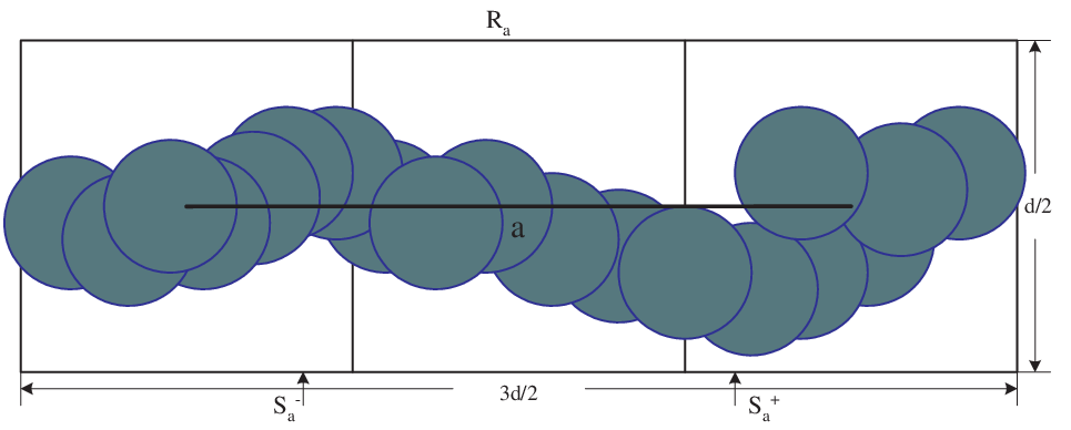
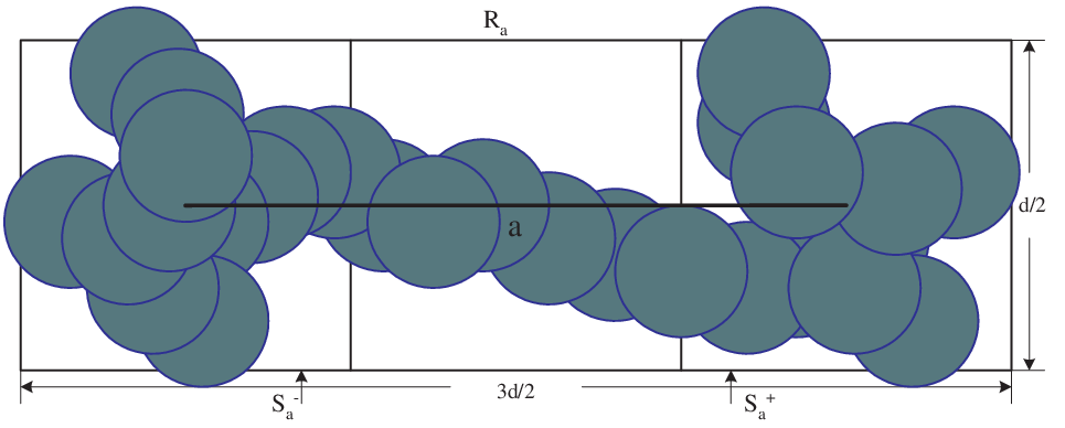
Further define event for edge in as the set of outcomes for which both of the following occur:
- (i)
occurs;
- (ii)
The left square and the right square are both crossed from top to bottom by connected components in .
If occurs, we say that rectangle is a complete rectangle, and edge is a complete edge. Let
Define similarly for all vertical edges by rotating the rectangle by . An example of a complete rectangle and a complete edge is illustrated in Figure 1-(b).
Note that the events are not independent in general. However, if two edges and are not adjacent, i.e., they do not share any common end vertices, then and are independent.
As illustrated in Figure 2, edges and are vertically adjacent to edge . It is clear that when events , and occur, event occurs. Moreover, since events , and are increasing events44 4 An event is called increasing if whenever graph is a subgraph of , where is the indicator function of . An event is called decreasing if is increasing. For details, please see [4, 2, 3]., according to the Fortuin-Kasteleyn-Ginibre (FKG) inequality [4, 2, 3],

According to Corollary 4.1 in [2], the probability converges to 1 as when is in the supercritical phase. In this case, converges to 1 as as well. Hence, converges to 1 as when is in the supercritical phase.
Now, define
| (6) |
where . Now choose the edge length of as . We further define complete events with respect to in the same way as we defined complete events with respect to .
Define event for each horizontal edge in as the set of outcomes for which the following condition is satisfied: The number of nodes of in is strictly less than
| (7) |
where , i.e., is the rectangle extended by 1 in all directions. Rectangle is shown in Figure 3. Note that .
Define similarly for all vertical edges by rotating the rectangle by . If occurs, we call rectangle and edge efficient. Let
Note that the events are not independent in general due to potential overlaps. However, if and two edges and are not adjacent, i.e., they do not share any common end vertices, then and are independent.

We say an edge in is open if and only if it is both complete and efficient, i.e., when events and both occur, and closed otherwise.
When occurs for edge in , no node of in has degree strictly greater than in . In addition, if satisfies (3), a node in with degree , , survives with a probability greater than or equal to in the degree-dependent failures model. On the other hand, for the independent random failures model, a node in survives with probability exactly equal to . Thus we can couple with so that the existence of crossings defined in events for implies the existence of crossings defined in events for . Hence, if edge of is open, there exists at least one left-to-right crossing and two top-to-bottom crossings in in . Therefore, a path of open edges in implies a connected component in . This is illustrated in Figure 4.
Although events and are not independent, we have
| (8) | |||||
Let be the number of nodes of in . Then has a Poisson distribution with mean
Note that . By Chebychev’s inequality, we have
| (9) | |||||
| (10) |
Now consider the dual lattice of . The construction of is as follows: let each vertex of be located at the center of a square of . Let each edge of be open if and only if it crosses an open edge of , and closed otherwise. It is clear that each edge in is open also with probability . Let
and choose edges in . Because the states (i.e., open or closed) of any set of non-adjacent edges are independent, we can choose edges among these edges such that their states are independent. As a result,
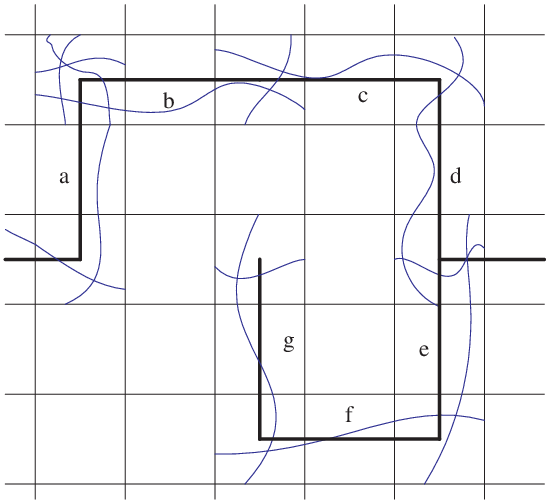
Now a key observation is that if the origin belongs to an infinite open edge cluster in , for which the event is denoted by , then there cannot exist a closed circuit (a circuit consisting of closed edges) surrounding the origin in , for which the event is denoted by , and vice versa. This is demonstrated in Figure 5.

Hence
Furthermore, we have
where is a closed circuit having length surrounding the origin, and is the number of such circuits.
By Lemma 3 in Appendix A, we have
| (11) | |||||
Because
we have , and hence . Thus the origin belongs to an infinite open edge cluster in with a positive probability. The existence of an infinite open edge cluster in implies the existence of an infinite connected component in , and this completes our proof for Theorem 1-(i). ∎
The first part of Theorem 1 provides a sufficient condition for to have an infinite component. The second part of Theorem 1 provides a sufficient condition for to have no infinite component. Thus, it provides a necessary condition for to have an infinite component. To show this, we use another mapping between the continuum model and a discrete percolation model.
Proof of Theorem 1-(ii): Map to a square lattice with edge length . Let the square centered at vertex with edge length be . Let and be the number of nodes of and in , respectively. We say is open if and only if either one of the following conditions holds:
- (i)
;
- (ii)
There is a link of crossing which directly connects two nodes of outside .
In Figure 6, we illustrate the possible examples of open squares in . If is open only because satisfies condition (ii), we say it is type-2 open; otherwise, we say it is type-1 open.

The probability that is type-1 open can be expressed as
| (12) | |||||
When is non-decreasing in , by Appendix B,
| (13) |
If (4) holds, we have . When is non-increasing in , by Appendix C,
| (14) |
If (5) holds, we have as well. Therefore, in both cases, we have .
If there is an infinite component in , there must exist an infinite path consisting of nodes in . Furthermore, this infinite path must pass through an infinite number of open squares in , as illustrated in Figure 7. This is because along the infinite path in , each square of contains at least one node of or is crossed by a link of that directly connects two nodes of outside .
Now choose a path in starting from the origin55 5 Note that the choice of the origin is arbitrary. having length . From Figure 6, we can see that a link from any given node in can go through at most three open squares in addition to the open square containing the given node. As a result, along the path, among every three consecutive open squares, there exists at least one type-1 open square. Thus, we have
| (15) |
Now
| (16) |
where is an open path in starting from the origin with length , and is the number of such paths. For a path in from the origin, the first edge has four choices for its direction, and all other edges have at most three choices for their directions. Therefore, we have
| (17) |
and
| (18) |
When , the RHS of (18) converges to 0 as . This implies that with probability 1, there is no infinite path starting from the origin (which is arbitrary) in . Therefore, with probability 1, there is no infinite component in either.∎
As an example of degree-dependent failures one may consider a strategy where an attacker sets a threshold and destroys all nodes having degree strictly greater than . Given and an integer , all nodes with degree strictly greater than and their associated links fail, and all other nodes remain operational. That is
| (19) |
Let the remaining graph be denoted by . By directly applying Theorem 1-(i), we know that there exists , such that when , is percolated.
We can also apply Theorem 1-(ii) to obtain a lower bound on the critical value of . By substituting (19) into (4), we see that if satisfies
| (20) |
then for any , is not percolated. Condition (20) can be simplified as
| (21) |
For any given , we can use (21) to find the critical value of . Figure 8 plots the maximal against satisfying (21).

IV Cascading Node Failures
As we pointed out before, in networks which carry load, distribute a resource or aggregate data, such as wireless sensor networks and electrical power networks, the failure of one node often results in the redistribution of the load from the failed node to other nearby nodes. If nodes fail when the load on them exceeds some maximum capacity or when the battery energy is depleted, then a cascading failure or avalanche may occur because the redistribution of the load causes other nodes to exceed their thresholds and fail, thereby leading to a further redistribution of the load.
Cascades have been used in social networks to model phenomena such as epidemic spreading, belief propagation, etc. Although they are generated by different mechanisms, cascades in social and economic systems are similar to a cascading failure in physical infrastructure networks [16, 17] in that initial failures can increase the likelihood of subsequent failures, leading to eventual dramatic global outages. Usually, such cascading failures are extremely difficult to predict, even when the properties of individual components are well understood. In [18, 19], the author investigate such cascading failures in social networks by modelling the problem as a binary decision percolation process on random networks where the links between distinct pairs of nodes are independent.
In contrast to previous work, we study cascading failures in large-scale wireless networks modelled by random geometric graphs. To our knowledge, this is the first investigation of cascading phenomena in networks with geometric constraints. In particular, we consider the following model. Consider a network modelled by a random geometric graph with , where an initial failure seed is represented by a single failed node. This initial failure seed is an exogenous event (shock) that is very small relative to the whole network. We are interested in whether this initial small shock can lead to a global cascade of failures, which is technically defined as follows.
Note that in characterizing cascading failure, the essential point is to assess whether the network has been affected in a global manner, rather than in an isolated local manner. For this reason, cascades cannot be easily characterized by, for instance, what percentage of the network nodes have failed. Instead, after some thought, one is led to the conclusion that percolation (the existence of an infinite failed component) is an appropriate notion with which to characterize cascading failures. Thus, we have the following definition.
Definition 2
A cascading failure is an ordered sequence of node failures triggered by an initial failure seed resulting in an infinite component of failed nodes in the network.
To describe cascading failures, we use the following simple but descriptive model. We assume that due to redistribution of the load, each node fails if a given fraction of its neighbors have failed, where the ’s are i.i.d. random variables with probability density function . The order of the failure sequence is then the topological order determined by the location of the initial failure and the threshold of each node .
Unlike the degree-dependent scenarios studied earlier, cascading failure processes exhibit dynamic evolution. This is illustrated in Figure 9. The simple network in Figure 9-(a) has nine nodes: , with failure thresholds .


At the beginning, as shown in Figure 9-(b), an initial failure occurs at node . Then, since and one of ’s three neighbors has failed, node fails. Similarly, node also fails. This is illustrated in Figure 9-(c). Since , does not fail until two of its five neighbors have failed (Figure 9-(d)). This process continues (Figure 9-(e)) until no further failures can occur in the network (Figure 9-(f)). The resulting network is denoted by , which, in this example, has failed nodes , , and operational nodes and . The ordered sequence of failures in this example is .
For two adjacent nodes and , we say that node ’s failure is caused by node ’s failure if and only if node ’s failure immediately follows node ’s failure in the ordered failure sequence. In the example of Figure 9, node ’s failure is caused by node ’s failure, and node ’s failure is caused by node ’s failure.
Now observe that the initial failure can grow only when some neighbor, say , of the initial failure seed has a threshold satisfying , where is the degree of . We call such a node vulnerable. The probability of a node being vulnerable is
| (22) |
where is the cumulative distribution function of . In the example of Figure 9, nodes , and are vulnerable.
When the initial failure seed is directly connected to a component of vulnerable nodes, all nodes in this component fail. The extent of the failure, and hence the resilience of the network, depends not only on the number of vulnerable nodes, but also on how they are connected to one another. In the context of this model, a cascade of failed nodes forms when the network has an infinite component of vulnerable nodes and the initial failure seed is either inside this component or adjacent to some node in this component.
On the other hand, if node has a threshold satisfying , where is the degree of , then node will not fail as long as at least one neighbor is operational. We call such a node reliable. Otherwise, if , we call node unreliable. For , the probability of a node being reliable is given by
| (23) |
For , we set . Intuitively, a node with no neighbors should be reliable, since it remains operational no matter what is, unless node itself is the initial failure. This also agrees with (23) by applying the convention . In the example of Figure 9, nodes , and are reliable, and all the other nodes are unreliable. Note that when two reliable nodes are adjacent and neither is an initial failure seed, no matter what else happens in the network, they remain operational. This is illustrated by nodes and in Figure 9. When a reliable node has only unreliable neighbors, node fails if and only if all its unreliable neighbors fail, unless node is the initial failure. We call such a reliable node an isolated reliable node.
The following theorem presents our main results on cascading failures in wireless networks. It provides a sufficient condition for the existence of an infinite component of vulnerable nodes, as well as a sufficient condition for the non-existence of an infinite component of unreliable nodes. The theorem asserts that when there exists an infinite component of vulnerable nodes and the initial failure is either inside this component or adjacent to some node in this component, then there is a cascading failure in . On the other hand, when there is no infinite component of unreliable nodes, then there is no cascading failure no matter where the initial failure is.
Theorem 2
(i) For any and with , there exists depending on such that if
| (24) |
then with probability 1, there exists an infinite component of vulnerable nodes in . Moreover, if the initial failure is inside this component or adjacent to some node in this component, then with probability 1, there is a cascading failure in .
(ii) For any with , if
| (25) |
where by convention, then with probability 1, there is no infinite component of unreliable nodes. As a consequence, with probability 1, there is no cascading failure in no matter where the initial failure is.
Proof: To prove (i), we view the problem as a degree-dependent node failure problem where a vulnerable node is considered “operational” and a non-vulnerable node is considered a “failure.” In this model, each node with degree fails with a probability . Then, by applying Theorem 1-(i) directly, we have for any and with , there exists such that if
| (26) |
then with probability 1, there exists an infinite component of vulnerable nodes in . If the initial failure is inside this component or adjacent to some node in this component, then there is a cascading failure in .
To prove (ii), we first show (a): if (25) holds, then with probability 1, there is no infinite component of unreliable nodes. We then show (b): if there is no infinite component of unreliable nodes, then with probability 1, there is no cascading failure no matter where the initial failure is.
To show (a), we apply the result of Theorem 1-(ii). Regard an unreliable node as “operational” and a reliable node as a “failure”. Then, —the probability of a node with degree being reliable—becomes the failure probability in the context of Theorem 1-(ii). Since is non-increasing in , we replace in (5) with and obtain (25). By Theorem 1-(ii), when (25) holds, with probability 1, there is no infinite component of unreliable nodes in the network.
In order to show (b), we will show that if there is a cascading failure, i.e., there is an infinite component of failed nodes, there must exist an infinite component of unreliable nodes in the network. Assume the initial failure takes place at node , and consider two cases: (1) node is an unreliable node or an isolated reliable node; (2) node is a non-isolated reliable node.
For case (1), if there is an infinite component of failed nodes in the network, all the failed nodes are either unreliable or isolated reliable. This is because non-isolated reliable nodes do not fail no matter what happens in the network. Furthermore, except for the initial failure, an isolated reliable node fails if and only if all its (unreliable) neighbors fail. This implies that except for the initial failure, the failure of any isolated reliable node does not cause any other failures. In other words, except for the initial failure, the failure of any unreliable node is caused by the failure(s) of other unreliable node(s). Thus, all the unreliable nodes in belong to the same component.
Now suppose there is only a finite number of unreliable nodes in . Then there must be an infinite number of isolated reliable nodes in . Note first that an isolated reliable node cannot be adjacent to another isolated reliable node by definition. Furthermore, as illustrated in Figure 10, each unreliable node cannot have strictly more than 6 isolated reliable neighbors. Therefore, it is impossible to have a finite number of unreliable nodes but an infinite number of isolated reliable nodes in . This contradiction ensures that the component of unreliable nodes in is infinite.

For case (2), a non-isolated reliable node fails if and only if (i) it is adjacent to the initial failure, (ii) not adjacent to any other reliable nodes, and (iii) all of its unreliable neighbors fail. We call a non-isolated reliable node satisfying condition (i)–(ii) an induced isolated reliable node. As illustrated in Figure 10, the number of induced isolated reliable nodes cannot be strictly greater than 6. Except for the initial failure and a finite number of induced isolated reliable nodes, all other failed nodes in are either isolated reliable or unreliable. Observe that as in the failure of an isolated reliable node, the failure of an induced isolated reliable node does not cause any other failures. In other words, except for the initial failure, the failure of any unreliable node is caused by the failure(s) of other unreliable node(s). Thus, all the unreliable nodes in belong to the same component. Then by the same argument for the first case, there must exist an infinite component of unreliable nodes in . ∎
V Simulation Studies
We illustrate degree-dependent node failures with two examples in Figure 11. The original network has nodes uniformly distributed in , and mean degree . In Figure 11-(a), . This function satisfies condition (3) and the remaining network of operational nodes still has a large connected component spanning almost the whole network, where empty circles represent failed nodes. In Figure 11-(b), , and . This function satisfies condition (4) and the remaining network of operational nodes consists of small isolated components.


In Figure 12, we illustrate cascading failures. Figure 12-(a) depicts a wireless network with nodes uniformly distributed in , and mean degree . Each node has a probability density function for the threshold , where for , and for . The ’s are assumed to be i.i.d. Figure 12-(b) depicts the largest component of vulnerable nodes (which are represented by empty circles) spanning the network. Figure 12-(c) indicates an initial failure caused by exogenous event, which is represented by a black solid node pointed to by an arrow. From Figure 12-(d), we see that the resulting network suffers from a cascading failure, where the failed nodes are represented by empty circles.


Figure 13 illustrates an example where no cascading failure occurs. The network is the same as the one shown in Figure 12-(a). Here, each node has a probability density function for the threshold , where for , and for . The ’s are assumed to be i.i.d. This function satisfies the condition (25). Figure 13-(a) shows that there is no large component of unreliable nodes (which are represented by empty circles) spanning the network. After the same initial failure as shown in Figure 12-(c) takes place, we see from Figure 13-(b) that the initial failure cause no other failures (failed nodes are represented by empty circles), and no cascading failure occurs in the network.


VI Conclusion
In this paper, we studied network resilience problems from a percolation-based perspective. To analyze realistic situations where the failure probability of a node depends on its degree, we introduced the degree-dependent failures problem. We model this phenomenon as a degree-dependent site percolation process on random geometric graphs. Due to its non-Poisson structure, degree-dependent site percolation is far from a trivial generalization of independent site percolation. Using coupling methods and renormalization arguments, we obtained analytical conditions for the occurrence of phase transitions within this model. Furthermore, in networks carrying traffic load, such as wireless sensor networks and electrical power networks, the failure of one node can result in redistribution of the load onto other nearby nodes. If these nodes fail due to excessive load, then this process can result in cascading failures. We analyzed this cascading failure problem in large-scale wireless networks, and showed that it is equivalent to a degree-dependent percolation process on random geometric graphs. We obtained analytical conditions for the occurrence and non-occurrence of cascading failures, respectively. To our knowledge, this work represents the first investigation of cascading phenomena in networks with geometric constraints.
Appendix A
The following lemma is similar to the one used in [10, 12, 4]. For completeness, we provide the proof here.
Lemma 3
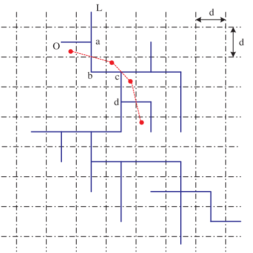
Given a square lattice , suppose that the origin is located at the center of one square. Let the number of circuits66 6 A circuit in a lattice is a closed path with no repeated vertices in . surrounding the origin with length be , where is an integer, then we have
| (27) |

Proof: In Figure 14, an example of a circuit that surrounds the origin is illustrated. First note that the length of such a circuit must be even. This is because there is a one-to-one correspondence between each pair of edges above and below the line , and similarly for each pair of edges at the left and right of the line . Furthermore, the rightmost edge can be chosen only from the lines . Hence the number of possibilities for this edge is at most . Because this edge is the rightmost edge, each of the two edges adjacent to it has two choices for its direction. For all the other edges, each one has at most three choices for its direction. Therefore the number of total choices for all the other edges is at most . Consequently, the number of circuits that surround the origin and have length must be less or equal to , and hence we have (27). ∎
Appendix B
By (12), the probability can be written as
| (28) | |||||
where is the indicator random variable indicating the failure of the -th node. Because is non-decreasing in , the event is an increasing event. Hence, according to the FKG inequality,
| (29) |
Since , all the nodes of in are adjacent to each other. Hence if there are nodes in , every node of in has degree greater than or equal to . In addition, since is non-decreasing in , we have
| (30) |
| (31) | |||||
Appendix C
Let be the shaded area shown in Figure 15. Then . Let be the number of nodes of in . Since and do not overlap, and are independent.

By (12), we can write as
| (32) | |||||
where is the indicator random variable indicating the failure of the -th node. Because is non-increasing in , the event is a decreasing event. Hence, according to the FKG inequality,
| (33) |
For any node inside , all of ’s neighbors are within . Given and , any node inside has degree less than or equal to . In addition, since is non-increasing in , we have
| (34) |
| (35) | |||||
References
- [1] E. N. Gilbert, “Random plane networks,” J. Soc. Indust. Appl. Math., vol. 9, pp. 533–543, 1961.
- [2] R. Meester and R. Roy, Continuum Percolation. New York: Cambridge University Press, 1996.
- [3] M. Penrose, Random Geometric Graphs. New York: Oxford University Press, 2003.
- [4] G. Grimmett, Percolation. New York: Springer, second ed., 1999.
- [5] B. Bollobás and O. Riordan, Percolation. New York: Cambridge University Press, 2006.
- [6] P. Gupta and P. R. Kumar, “Critical power for asymptotic connectivity in wireless networks,” in Stochastic Analysis, Control, Optimization and Applications: A Volume in Honor of W. H. Fleming, pp. 547–566, 1998.
- [7] L. Booth, J. Bruck, M. Franceschetti, and R. Meester, “Covering algorithms, continuum percolation and the geometry of wireless networks,” Annals of Applied Probability, vol. 13, pp. 722–741, May 2003.
- [8] M. Franceschetti, L. Booth, M. Cook, J. Bruck, and R. Meester, “Continuum percolation with unreliable and spread out connections,” Journal of Statistical Physics, vol. 118, pp. 721–734, Feb. 2005.
- [9] O. Dousse, P. Mannersalo, and P. Thiran, “Latency of wireless sensor networks with uncoordinated power saving mechniasm,” in Proc. ACM MobiHoc’04, pp. 109–120, 2004.
- [10] O. Dousse, M. Franceschetti, and P. Thiran, “Information theoretic bounds on the throughput scaling of wireless relay networks,” in Proc. IEEE INFOCOM’05, Mar. 2005.
- [11] O. Dousse, F. Baccelli, and P. Thiran, “Impact of interferences on connectivity in ad hoc networks,” IEEE Trans. Network., vol. 13, pp. 425–436, April 2005.
- [12] O. Dousse, M. Franceschetti, N. Macris, R. Meester, and P. Thiran, “Percolation in the signal to interference ratio graph,” Journal of Applied Probability, vol. 43, no. 2, 2006.
- [13] Z. Kong and E. M. Yeh, “Distributed energy management algorithm for large-scale wireless sensor networks,” in Proc. ACM MobiHoc’07, Montreal, Canada, Sep. 2007.
- [14] Z. Kong and E. M. Yeh, “Connectivity and latency in large-scale wireless networks with unreliable links,” in Proc. IEEE INFOCOM’08, Phoenix, AZ, April 2008.
- [15] Z. Kong and E. M. Yeh, “On the latency of information dissemination in mobile ad hoc networks,” in Proc. ACM MobiHoc’08, Hong Kong SAR, China, May 2008.
- [16] D. N. Kosterev, C. W. Taylor, and W. A. Mittelstadt, “Model validation for the august 10, 1996 wscc system outage,” IEEE Trans. on Power Systems, vol. 14, pp. 967–979, Aug. 1999.
- [17] M. L. Sachtjen, B. A. Carreras, and V. E. Lynch, “Disturbances in a power transmission system,” Physics Review E, vol. 61, pp. 4877–4882, May 2000.
- [18] D. J. Watts, “A simple model of global cascades on random networks,” Proc. Natl. Acad. Sci. USA, vol. 99, pp. 5766–5771, 2002.
- [19] M. E. J. Newman, “The structure and function of complex networks,” SIAM Review, vol. 45, pp. 167–256, 2003.
- [20] J. Quintanilla, S. Torquato, and R. M. Ziff, “Efficient measurement of the percoaltion threshold for fully penetrable discs,” Physics A, vol. 86, pp. 399–407, 2000.
- [21] R. Cohen, K. Erez, D. ben Avraham, and S. Havlin, “Resilience of the internet to random breakdowns,” Phys. Rev. Lett., vol. 85, pp. 4626–4628, Nov. 2000.
- [22] D. S. Callaway, M. E. J. Newman, S. H. Strogatz, and D. J. Watts, “Network robustness and fragility: percolation on random graphs,” Phys. Rev. Lett., vol. 85, pp. 5468–5471, Dec. 2000.
- [23] M. E. J. Newman, S. H. Strogatz, and D. J. Watts, “Random graphs with arbitrary degree distributions and their applications,” Phys. Rev. E, vol. 64, no. 026118, 2001.
- [24] P. B. Godfrey and D. Ratajczak, “Naps: Scalable, robust topology managemen in wireless ad hoc networks,” in Proc. ACM IPSN’04, April 2004.
- [25] V. Strassen, “The existence of probability measures with given marginals,” Ann. Math. Statist., vol. 36, no. 2, pp. 423–439, 1965.