A reliable cluster detection technique using photometric redshifts: introducing the 2TecX algorithm
Abstract
We present a new cluster detection algorithm designed for finding high-redshift clusters using optical/infrared imaging data. The algorithm has two main characteristics. First, it utilises each galaxy’s full redshift probability function, instead of an estimate of the photometric redshift based on the peak of the probability function and an associated Gaussian error. Second, it identifies cluster candidates through cross-checking the results of two substantially different selection techniques (the name 2TecX representing the cross-check of the two techniques). These are adaptations of the Voronoi Tesselations and Friends-Of-Friends methods. Monte-Carlo simulations of mock catalogues show that cross-checking the cluster candidates found by the two techniques significantly reduces the detection of spurious sources. Furthermore, we examine the selection effects and relative strengths and weaknesses of either method. The simulations also allow us to fine-tune the algorithm’s parameters, and define completeness and mass limit as a function of redshift. We demonstrate that the algorithm isolates high-redshift clusters at a high level of efficiency and low contamination.
Keywords:
methods: data analysis – galaxies: clusters: general – techniques: photometric1 Introduction
Remote galaxy clusters have been used in a wide range of cosmological and astrophysical contexts. In cosmology, clusters can be used to trace the large-scale structure of the universe. Their number density, as a function of redshift, can place constraints on various cosmological quantities. These include the mass density of the universe, the amplitude of the initial density fluctuations, and the cosmic growth function. Clusters also act as astrophysical laboratories for understanding the formation and evolution of galaxies and their environments. This is because the deep potential well of a cluster causes it to retain virtually all its gas and galaxies, allowing a detailed inspection of the interaction between both. It is therefore desirable to have a large, homogeneous catalogue of clusters at a range of redshifts in the universe.
Abell compiled the first large cluster catalogue, in which clusters were selected in a consistent manner (Abell 1958; Abell, Corwing & Olowin 1989). This catalogue was created from photographic observations, which suffer from non-linear plate-to-plate sensitivity variations and considerably large photometric errors (Sutherland 1988). Furthermore, the clusters were found by eye which poses problems for the objectivity and completeness of the cluster sample and the line-of-sight projections contaminating it (e.g. Lucey 1983; van Haarlem, Frenk & White 1997). A particularly important advance has come from optical galaxy surveys using large arrays of CCD detectors, such as the relatively shallow (z 0.4) Sloan Digital Sky Survey (SDSS) (e.g Goto et al. 2002; Kim et al. 2002; Miller et al. 2005). A recent large-scale cluster catalogue using the SDSS was initiated by Koester et al. (2007a,b), detecting clusters at . There have been numerous smaller-area surveys to much higher redshift, as for instance the Palomar Distant Cluster Survey (Postman et al. 1996); the ESO Imaging Survey (Lobo et al. 2000); and the Red Sequence Cluster Survey (Gladders & Yee 2005).
Optical cluster surveys were limited for a long time to clusters at , due to the fact that the cluster galaxy population largely consists of early-type red galaxies. At redshifts of , the 4000 Å break moves into infrared bands, complicating the detection of these galaxies in optical surveys. A crucial development has been the advent of wide-field infrared cameras. Deep, large-area infrared studies have already become available from the Wide Field Infrared Camera (WFCAM) on the United Kingdom Infra-Red Telescope (UKIRT) and the Spitzer space telescope and will shortly be available on the Visible and Infrared Survey Telescope for Astronomy (VISTA).
There exist many methods for detecting clusters in optical imaging surveys. The problem is somewhat easier for galaxy datasets with spectroscopic redshifts owing to the accurate knowledge of each galaxies distance. However, spectroscopy is time consuming and approximate redshifts can be calculated via photometric redshift estimation. This technique is considerably less precise which makes looking for structure less straightforward. A successful photometric method for finding clusters is to use deep optical imaging data that span the rest frame 4000 Å break (Gladders & Yee, 2000). This is motivated by the observation that cluster early-type galaxies form a characteristic red sequence comprising the brightest, reddest galaxies at a given redshift. The colour of this red sequence also provides an estimate of the redshift of the detected cluster, thereby reducing projection effects (e.g. Gladders and Yee, 2005). However, at high redshift there is not yet substantial evidence whether all clusters do indeed show a red sequence. Merely selecting by this characteristic could be introducing a large bias against younger clusters with ongoing star-formation.
In this paper we present a new cluster detection method, specifically designed to detect high-redshift clusters using optical/infrared imaging data. In Section 2 we describe the cluster detection algorithm step by step. Section 3 contains details of the creation of mock catalogues, along with simulations for parameter optimisation and to determine the completeness and contamination by spurious sources. Section 4 is a summary of the algorithm and its performance on the set of simulations. We assume throughout this paper that , and a , cosmology. All magnitudes are given in the Vega system.
2 2TecX: a new cluster detection algorithm
Optical cluster surveys using selection methods based on photometric redshifts often suffer from two common problems: (i) projection effects of fore- and back-ground galaxies and (ii) determining the reality of detected clusters. The former issue arises because photometric redshifts, as opposed to spectroscopic redshifts, typically have errors of the order of ; furthermore the photometric redshift probability functions (z-PDFs) are often significantly non-Gaussian and can for instance show double peaks. The second issue – the occurrence of spurious cluster detections – is due to sensitivity of the detection algorithm to noisy data. To create a cluster catalogue a compromise needs to be made between completeness and contamination: we want to include as many clusters as possible above a certain mass limit, without suffering from contamination by spurious sources. It is important to understand the completeness and efficiency of cluster finders.
To address these two problems, we create a new cluster-detection algorithm that is characterised by two main improvements upon previous work: (i) the cluster-detection algorithm utilises the full z-PDF instead of a single best redshift-estimate with an associated Gaussian error; (ii) we maximise the efficiency by cross-checking the output of two substantially different cluster detection methods.
The algorithm is divided into six steps, described in more detail in the following subsections and shown schematically in Fig. 1:
- 1.
Determining z-PDFs for all galaxies in the field.
- 2.
Creating 500 Monte-Carlo (MC) realisations of the three-dimensional galaxy distribution, based on the galaxy z-PDFs.
- 3.
Dividing each MC-realisation into redshift slices of over the range .
- 4.
Detecting cluster candidates in each slice of all MC-realisations using independent Voronoi Tessellation (VT) and Friends-Of-Friends (FOF) methods.
- 5.
Mapping the probability of cluster candidates for both methods based on the number of MC-realisations in which they occur.
- 6.
Cross-checking the output of the VT and FOF methods to arrive at the final cluster-catalogue.

2.1 Redshift probability distribution functions
The photometric redshifts of Van Breukelen et al. (2006, henceforth VB06), who first applied our cluster-detection algorithm to optical/infrared imaging data, were created by an adapted version of Hyperz (Bolzonella et al. 2000), using a set of Spectral Energy Distributions (SEDs) generated with GALAXEV (Bruzual & Charlot 2003). Hyperz estimates photometric redshifts by fitting a range of SED templates to the measured fluxes in several photometric bands. The shape of the SEDs are determined by various parameters, such as the rate of ongoing star-formation, the age of the galaxy, the metallicity, and the reddening due to extinction. A redshift probability distribution function is constructed by calculating the probability of the best-fitting set of parameters at each redshift. Thus the z-PDF does not reflect the probability with redshift for a single template, but rather for the total set of templates. The location of the maximum of the z-PDF is taken as the photometric redshift and an error can be estimated by fitting a Gaussian profile to the probability peak. However, this does not take into account the often non-Gaussian and sometimes double-peaked nature of the z-PDF. These can arise because different features of the spectrum can be confused (for example the 4000 Å break and the Lyman- break at Å) or various templates can give solutions of comparable probability at different redshifts. We therefore do not use a best-estimate photometric redshift, but take the entire z-PDF into account in our cluster search. The output of our adapted Hyperz program is the marginalised likelihood associated with each step in redshift space for each galaxy. However, the 2TecX algorithm can be applied to any photometric redshift dataset that contains a z-PDF for every galaxy.
2.2 The Monte-Carlo realisations and redshift slicing
To include the entire z-PDF of each galaxy into our cluster-detection algorithm, we create 500 MC-realisations of the three-dimensional galaxy distribution by randomly sampling each z-PDF. We chose the number of realisations as a compromise between computational time and sampling accuracy of the z-PDF. We now have 500 cubes of RA, Dec, and , where each galaxy is represented by a single point. The shape of the z-PDF of each galaxy determines its position in the cubes; if the peak in the probability distribution function is sharp the galaxy will occur in all cubes at approximately the same redshift whereas if the z-PDF consists of two equally probable peaks the galaxy will be placed at either redshift in an equal number of cubes.
Next, we divide each MC-realisation into redshift slices of a width, , approximately equal to the photometric redshift error, . If the width is chosen to be significantly smaller, clusters can be undetected due to the distribution of their member galaxies over too many redshift slices; if it is chosen substantially larger, many spurious sources will be found owing to projection effects. In this paper we use , as this is the approximate photometric redshift error of VB06.
2.3 Two cluster selection methods
We now have 500 MC-realisations of the three-dimensional galaxy distribution, each divided into redshift slices. In the next step, the algorithm applies two cluster selection methods independently to each redshift slice of all the MC-realisations. The two methods used are Voronoi Tessellation and Friends-Of-Friends, which are described in more detail below.


2.3.1 Voronoi Tessellations

The VT technique divides a field of galaxies into Voronoi Cells, each containing one object: the nucleus. All points that are closer to this nucleus than any of the other nuclei are enclosed by the Voronoi Cell (see Fig. 2). This technique was first applied to the modelling of large-scale structure (e.g. Icke & van de Weygaert 1987) but has more recently been used in cluster detection (Ebeling & Wiedenmann 1993; Kim et al. 2002; Lopes et al. 2004). One of the principal advantages of the VT method is that the technique is relatively unbiased as it does not look for a particular source geometry (e.g. Ramella 2001). The parameter of interest is the area of the VT cells, the reciprocal of which translates to a density. Overdense regions in the plane are found by fitting a function to the density distribution of all VT cells in the field; cluster candidates are the groups of cells of a significantly higher density than the mean background density.
Kiang (1966) showed that, for randomly (Poissonian) distributed points, the differential distribution function of the cell area is of the following form:
| (1) |
Here is the dimensionless cell area in units of the average cell area: , where is the total number of cells. is the Gamma Function. The cumulative distribution function for the cell area is the integral of Eq. 1, namely:
| (2) |
The density of the VT cells is the reciprocal of Eq. 2:
| (3) |
Here is the dimensionless cell density (the inverse of the cell area) in units of the mean cell density:
| (4) |
In our algorithm, we approximate the density distribution of the background galaxies by a Poissonian distribution, allowing us to fit the cumulative density distribution of the data with a function of the form of Eq. 3. Note however that due to this approximation, the derived equations in this section do not reflect the exact statistics of the galaxy background. However by tuning the parameters through simulations (see Section 3.4), the resulting statistical approximation is adequate for our purposes.
The aim of the fitting procedure is to calculate the average density of the background cells, so we can subsequently impose a lower limit on the density of the cells that are caused by clustering. However, we can only fit the function to the lower-density end of the distribution which is not influenced by the cells in the overdense regions. Therefore we first estimate the background density by inspecting the histogram of the cell densities.

Fig. 3 shows the VT cell density distribution in a field of 2000 randomly distributed background galaxies, containing a structure of 100 galaxies in the centre with a Gaussian density profile with (see also Fig. 4). If we assume the peak in this histogram is not polluted by the overdense regions, the form of Eq. 1 dictates that the average background density is times the density at which the peak occurs. This can be shown by requiring that the derivative of Eq. 1 is zero and applying Eq. 4. Next we can fit the predicted cumulative distribution function to the cumulative distribution function of our data where , as suggested by Ebeling & Wiedenmann (1993). Once the exact background density is known, we isolate all cells with ; is the density at which overdense regions start to contribute significantly to the cumulative density distribution. Adjoining high-density cells are grouped together; if the group consists of a number greater than a certain lower limit, it is taken to be a cluster candidate. Fig. 4 illustrates this procedure: the Voronoi tessellated field is shown on the left along with the high-density groups and the cluster candidate; on the right the cumulative density distribution is plotted. The limiting number of galaxies, , can be calculated by setting a lower limit to : the expected number of groups caused by background fluctuations. Ebeling & Wiedenmann (1993) derived this quantity as described below in Eqs. 5 - 8. Note that we use the lower case notation for numbers of individual Voronoi Cells (each representing a galaxy), and the capital for numbers of high-density groups of Voronoi Cells (corresponding to cluster candidates).
The expected number of groups caused by background fluctuations, comprising a certain number of galaxies above the background level, , can be written as:
| (5) |
where is the minimum density cut-off value used to select high-density cells, and is the number of background galaxies expected in the field. The latter comes directly from the fitted average background density by recognising that and therefore , where is the total area of the survey field. is the number of high-density groups with no extra galaxies above the background level; and have been shown by Ebeling & Wiedenmann (1993) to obey the following empirical relations:
| (6) |
| (7) |
Integrating the function given in Eq. 5 from the limiting number of galaxies to infinity gives the expected number of groups caused by background fluctuations with :
| (8) |
Thus, the limiting number of galaxy members in a group considered to be a cluster candidate is:
| (9) |
The number of galaxy members, , is determined for each group and compared to . Note that needs to be corrected for the background number density of galaxies, which is calculated by dividing the total area of the group, , by the average cell area: . The Voronoi Tessellations method thus has two parameters for which a value needs to be chosen: the minimum cut-off dimensionless density and the maximum expected number of groups caused by background fluctuations, .

2.3.2 Friends-Of-Friends
Friends-Of-Friends algorithms are commonly used in spectroscopic galaxy surveys (e.g. Tucker et al. 2002; Ramella et al. 2002). A variant of this algorithm utilising photometric redshifts was proposed by Botzler et al. (2004). They create redshift slices for their data cube and place the galaxies into the redshift slices according to their photometric redshift and error; objects with large errors are removed. The algorithm then calculates the distance of one galaxy to all others in the redshift slice, and groups the galaxies that are closer to each other than a given linking distance, (‘friends’). Next it calculates the distance from the new galaxies in the group (the ‘friends’) to all other galaxies in the slice and adds those that are within the linking distance (‘friends-of-friends’). The group is complete when there are no more galaxies to be found within the linking distance to any of the group members. If the group comprises a number of galaxies above a specified minimum number, , it is a cluster candidate. Cluster candidates in separate redshift slices that contain one or more identical galaxy members are linked up as one and the same cluster candidate.
Our Friends-Of-Friends algorithm is broadly similar to that of Botzler et al. (2004). However, we have made three key improvements, which will be discussed below.
First, to speed up the computational efficiency, we apply Delaunay Triangulation (Delaunay, 1934) to the field of galaxies in the redshift slice to identify each galaxy’s nearest neighbours (‘Delaunay neighbours’). This procedure uses the ‘divide-and-conquer’ method described in Lee & Schachter (1980), which has a very short computational run time. Hereby our computation time is greatly reduced as once we have completed the triangulation, there is no need to calculate the distance from each galaxy to every other galaxy in the field, but only to determine the distance to each galaxy’s Delaunay neighbours. Fig. 5 demonstrates the principle of Delaunay Triangulation: each galaxy is connected to its nearest neighbours, forming triangles whose circumcircle contains no other galaxies than the ones that form the vertices of the triangle itself.
When the triangulation is complete, a random galaxy is chosen and the proper distance, , to its neighbours as linked by the Delaunay triangulation, is calculated from:
| (10) |
where is the angular distance of the redshift slice, and is the angle between the galaxies and in the tangent-plane approximation:
| (11) |
In this equation and are the RA and Dec of the galaxies in units of degrees. Any neighbours for which are dubbed ‘friends’ and are added to the group. Next, the previous step is repeated for the new ‘friends’, taking only the galaxies into account that are not yet members of the group. When there are no more ‘Delaunay neighbours’ of any members of the group within linking distance, an as yet unanalysed galaxy is chosen and the whole process is repeated. This is illustrated by Fig. 6, where the Delaunay Triangulation is shown of a galaxy field with an overdensity superimposed and the iterations of the Friends-Of-Friends process are colour-coded. When all groups have been found in the redshift slice, only those with a number of galaxies greater than are retained. Evidently, the two parameters in FOF for which a value needs to be chosen are and .
The second important difference between our algorithm and previous ones in the literature, such as Botzler et al. (2004), is the way we place the galaxies in the redshift slices. As we sample the full z-PDF to create MC-realisations of the three-dimensional galaxy distribution, we do not need to assign errors to individual galaxy redshifts. An object with a large redshift error will be distributed throughout many different slices in the 500 MC-realisations, and therefore not yield a significant contribution to the cluster candidates it is potentially found in. Thus there is no need to remove objects with large errors from the catalogue and no additional bias is introduced against faint objects with noisier photometry.
The third modification to existing algorithms is the way we link up cluster candidates throughout the redshift slices. Instead of comparing individual galaxies in the clusters and linking up the clusters with corresponding members (see Botzler et al. 2004), we use probability maps of all redshift slices to locate likely cluster regions. This is discussed in Section 2.4.
2.4 Probability maps and cross-checking

Once the two cluster selection methods have determined the cluster candidates in the redshift slices for all MC-realisations, we combine the MC-realisations to create probability maps for both methods for each redshift slice. These maps are created by calculating the extent of all cluster detections in RA and Dec according to the positions of the cluster members. The regions of the field that are found to be in a cluster in many MC-realisations are high-probability cluster locations. Fig. 7 shows an example of a probability map: the VT cluster candidates in this slice at are contoured and coloured, with black through to red indicating low to high probability.
Since the error on the photometric redshifts of the galaxies is usually larger than the width of the redshift slices, each cluster candidate is typically found in several adjoining slices. We join the cluster candidates that occur in the same location in several slices by locating the peaks in the probability maps and inspecting the area within their contours in the adjoining redshift slices for cluster candidates. This procedure is carried out as follows: per redshift slice, starting at the highest detected contour level, we calculate the positions of the cluster contours and determine their ’centres of mass’, where each point within the contour is assigned an equal ’mass’. Next, we inspect the contours one level down, and verify if any of these are unoccupied by any of the previously found centres. If so, this is labelled a new cluster (of a lower probability). We continue until we have inspected all contour levels down to 0.05 (or 5% of the number of MC realisations) in all redshift slices. Finally, we join each cluster centre to the cluster centres in adjoining redshift slices that lie within 0.5 Mpc in projected distance. Fig. 8 shows the cumulative number of MC-realisations versus redshift for one cluster candidate. The redshift limits of the linking procedure are placed at the slices where the cluster candidate is no longer found in a significant number of MC-realisations (i.e. of the MC realisation). The final cluster redshift is determined by taking the mean of the redshift slices, weighted by the number of MC-realisations in which the candidate is detected.

We assign a reliability factor to each cluster by counting the total number of MC-realisations in which it occurs in any of the linked-up redshift slices, and dividing this by the total of 500 realisations. This means that if a cluster candidate occurs in four slices in a single realisation, it is only counted once. Therefore the maximum number of realisations in which it is counted is 500, in which case we would have . To create the final cluster catalogue, we cross-check the output of the two detection methods and select only those clusters that have been found by both VT and FOF with a reliability factor above a suitable limit. This parameter is dependent on the accuracy of the photometric redshifts, and the completeness and efficiency of both detection methods. The higher the chosen limit, the more efficient yet the less complete the final cluster catalogue will be. The best level of is determined by simulating mock catalogues, taking into account the characteristics of the data to be used. Below we describe the results of running the 2TecX algorithm on our simulated catalogues. Based on these, VB06 used a value of to obtain a reliable cluster catalogue at .
3 Simulations
3.1 Mock catalogue characteristics
To test the behaviour of the cluster-detection algorithm and to determine the optimal values of the parameters we run a set of simulations on mock catalogues. These catalogues need to mimic as closely as possible the data to which the algorithm will be applied. VB06 describe the application of our algorithm to a combined optical/infrared catalogue on the Subaru-XMM-Newton Deep Field (SXDF) consisting of Subaru SuprimeCam data; United Kingdom InfraRed Telescope (UKIRT) Wide Field CAMera (WFCAM) data from the UKIRT Infrared Deep Sky Survey (UKIDSS); and 3.6 and 4.5 bands data from the Spitzer InfraRed Array Camera (IRAC). Our mock catalogues are designed to have the same area and -band limiting magnitude as the data catalogue of VB06. Furthermore, when a galaxy’s z-PDF is needed, this is randomly drawn from the collection of z-PDFs used by VB06 that peak at the position of the simulated galaxy’s redshift. Thus the z-PDFs of the simulated data accurately reflect the photometric redshift error and the functional form of the z-PDFs in the real data catalogue.

3.2 Simulating the galaxy background
We create catalogues with a galaxy background distribution randomly placed in the field with (neglecting clustering of both the background and the clusters). The galaxy luminosities and number densities are determined by the -band Schechter luminosity function of Cole et al. (2001) with , , and . To obtain the correct value for we added (Hewett et al. 2006) to Cole’s original value to account for the difference between the -band filters of WFCAM and 2MASS (used by Cole et al. 2001). Also, we assume passive evolution of the luminosity function (e.g. Gardner et al. 1996). We calculate the + (evolution and redshifting) correction to at all redshifts by using GALAXEV to create a stellar population synthesis SED. The SED consists of a star-burst at , exponentially decaying with , and has solar metallicity. The creation of the background catalogues is done in the following steps:
- 1.
We slice the three-dimensional field into redshift slices of over which we assume the luminosity function to be constant.
- 2.
For each slice, we calculate the volume (), determined by the angular size of the field and the redshift limits, and the + corrected .
- 3.
The number of simulated galaxies in the slice is calculated according to the luminosity function:
(12) and
(13) where is a dimensionless luminosity.
- 4.
Luminosities are assigned to all galaxies according to the luminosity function of Eq. 13, and the absolute magnitudes are determined with:
(14) - 5.
The galaxies are randomly placed in redshift, RA, and Dec within the slice according to a uniform distribution.
- 6.
The apparent magnitudes of the simulated galaxies are calculated:
(15) where is the luminosity distance to the galaxy in parsec. We now impose a magnitude limit of to match the 5- limit of the data catalogue of VB06. Only the galaxies with are retained in the mock catalogue.
The number of galaxies as a function of magnitude in each mock catalogue is entirely consistent with the number counts in the data catalogue up to the 5- limit, as is shown in Fig. 9.
3.3 Adding mock clusters to the catalogue
We superimpose simulated clusters on the background catalogue. To create the mock clusters we take the following steps:
- 1.
We choose a total cluster mass (including dark matter) and a mass-to-light ratio of (Rines et al. 2001) which is assumed constant in terms of L∗ (a quantity we assume to evolve passively with redshift). To deduce the total luminosity of the cluster in -band we calculate:
(16) and therefore the total dimensionless luminosity in units of is:
(17) Here is the -band magnitude of the sun and is taken from the cluster luminosity function derived by Lin, Mohr & Stanford (2004), who found , , and . Again we assume passive evolution of the cluster luminosity function with a formation redshift of .
- 2.
We calculate the number of galaxies in the cluster by using Eq. 12 and recognising that:
(18) Together this gives:
(19) or in units of :
(20) Luminosities are assigned to the galaxies according to the luminosity function of Lin et al. (2004).
- 3.
The galaxies are spatially distributed within the cluster according to an NFW profile (Navarro, Frenk & White, 1997) with a cut-off radius of 5 Mpc. Assuming galaxies to be perfect tracers of the dark matter, the galaxy number density in the two-dimensional projected NFW profile is (Bartelmann 1996):
(21) Here , where is the radius in projection. The scale radius is related to (the radius of the circle whose density is 200 times the critical density of the Universe) via . The concentration factor has been determined from numerical simulations by Dolag et al. (2004) to obey the empirical relation:
(22) with , , and .
The radius is determined by the total mass of the cluster:(23) where for a flat Universe:
(24) In this equation is expressed in , and is the gravitational constant. When simulating elliptical clusters, we use the radius for the profile over one axis, and the radius over the other axis, where is the ellipticity expressed in minor axis over major axis.
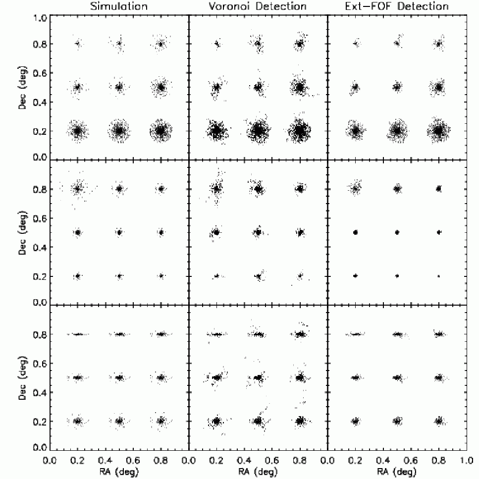
Figure 11: Mock clusters as recovered by the Voronoi Tessellations and Friends-Of-Friends algorithms. The left panel shows the distribution of cluster galaxies in the mock catalogues; note that the background galaxies have been removed from the plot for clarity. The middle panel shows the clusters as recovered by the VT method, whereas the right panel shows the clusters as recovered by the FOF method. The three simulated cluster fields (top to bottom) are identical to the ones in Fig. 10, where the top panel contains the clusters of varying mass, the middle panel the clusters at varying redshift, and the bottom panel the clusters of varying ellipticity. - 4.
The redshifts of the cluster galaxies are randomly offset from the cluster redshift according to a Gaussian distribution with , which is the expected photometric redshift error (see VB06). This error is much larger than the contribution of the velocities of the galaxies within the cluster, which allows us to neglect the latter.
- 5.
Again, we apply the magnitude limit of to the apparent magnitudes of the cluster galaxies to obtain the final catalogue.
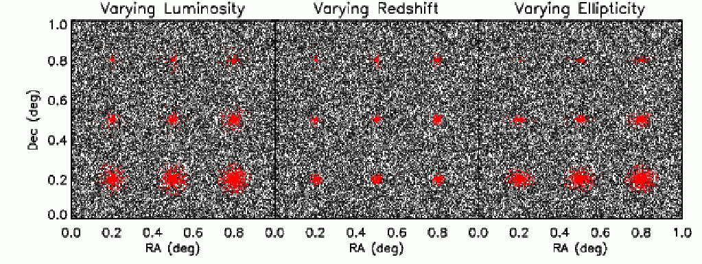
We create different types of mock cluster catalogues: (i) a set of clusters with varying mass or total luminosity at fixed redshift, (ii) a set of clusters of fixed mass at varying redshifts, and (iii) a set of clusters of fixed mass and redshift, but with varying ellipticity. The varying mass and redshift catalogues are created such that each combination of mass and redshift is represented and all catalogues are recreated randomly ten times. In Fig. 10 we show the distribution of galaxies in our three types of catalogue: on the left nine clusters at with total luminosities of = 10, 20, 30, 40, 50, 100, 150, 200, 300 ; in the middle nine clusters of at = 0.2, 0.4, …, 2.0; on the right nine clusters of at , with ellipticity = 0.1, 0.2, …, 1.0 at a position angle (PA) of 0∘.
3.4 Simulation results

The aim of the simulations is to explore the behaviour of the FOF and VT detection methods, and to optimise the algorithm’s parameters. The VT and FOF methods each have two free parameters. For FOF these are the linking distance in proper coordinates, , and the minimum number of galaxies in a cluster, . Guided by Botzler et al. (2004) we experimented with values between 0.125 Mpc 0.175 Mpc, and . For VT the parameters are the expected number of groups due to background fluctuations, , and the lower limit on the cell density, . We followed the method of Ebeling & Wiedenmann (1993) and set to 0.1. For we tried values of , where equates to the mean cell density of the field. We use the parameters that give the best completeness of detected clusters whilst keeping the contamination low: Mpc, , and .
Now that we have determined each algorithm’s optimal parameters, we test the behaviour of the cluster detection routine by trying to recover the clusters of the three different types of mock catalogues described in the previous section. Fig. 11 shows an example: the left panel contains the simulated clusters, the middle panel the clusters recovered by VT, and the right panel the clusters recovered by FOF. Note that in the left panel the background galaxies have been removed for clarity; naturally they were present when running the cluster detection algorithm.

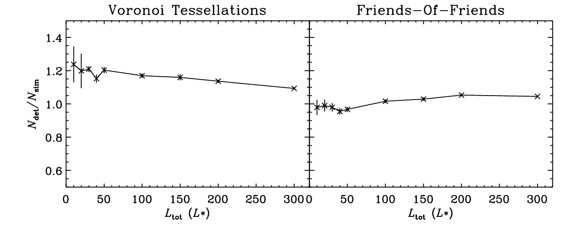
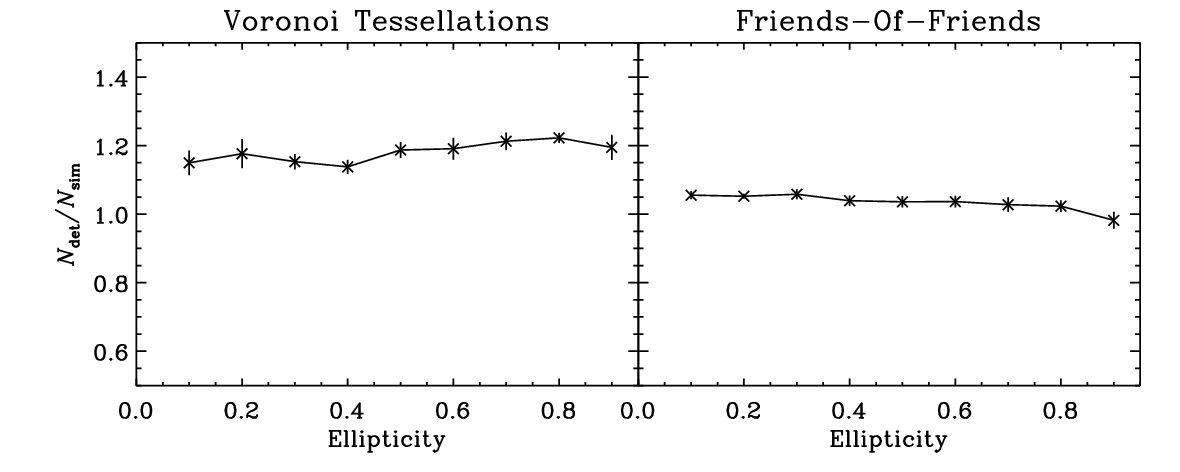
Both methods recover all clusters satisfyingly; there is no obvious bias to cluster morphology as the elliptical clusters are recovered very well by both methods. However, the recovered shape of the clusters differs for both methods: VT tends to pick up more background galaxies at the edges of the clusters as the number of recovered cluster members, , in any cluster is sensitive to the local field density. By contrast, the galaxy members recovered by FOF are more centrally concentrated; the total number of recovered galaxies per cluster is consistent throughout the random realisations of the catalogues. This is illustrated in Fig. 12 which shows the fraction of recovered cluster galaxies by both methods for the types of catalogues shown in Fig. 11. The number of simulated cluster galaxies is determined both by the cluster’s mass and the magnitude limit at its respective redshift. The difference in both methods is particularly noticeable in the middle panel of Fig. 12, where the recovered fraction of cluster galaxies is shown versus redshift. As there are few background galaxies in the high-redshift slices, the fraction of detected galaxies per cluster declines in the FOF method as there is a smaller chance of finding background galaxies within the linking distance. However, the fraction of detected cluster galaxies remains constant in VT because the algorithm’s parameters to estimate an overdensity are scaled to the background density, which negates the effect of having less background galaxies in the redshift slice.
With the chosen set of parameters we can calculate the detection completeness as a function of redshift for clusters of varying total mass. Fig. 13 shows the result: clusters of mass are detected with a high completeness up to , whereas the lower-mass clusters show rapidly declining completeness at lower redshifts. The FOF algorithm achieves a higher completeness than VT for clusters of equal mass; however the contamination of spurious sources is found to be higher.
The effects of contamination of the individual detection methods can be greatly reduced by cross-checking the output of both methods. Since both methods use different measures to isolate clusters (galaxy density in VT versus separation in FOF) the false detections in both do not typically coincide. Therefore by cross-checking the output of the two methods and choosing a sensible lower limit for the reliability factor , the spurious sources due to biases in the algorithms disappear, leaving only chance galaxy groupings. Fig. 14 is an example of this: it shows the cluster candidates found in all redshift slices by both methods; although there are spurious detections both from VT and FOF, none are found by both. In Fig. 15 the efficiency, in terms of the number of real clusters as a fraction of the total detected clusters, in all 30 mock catalogues is plotted for either method. Here all clusters with are included. The median efficiency is 0.8 for both methods; none of the spurious sources are detected by both techniques. Note however that this is purely an upper limit to the efficiency: for a true estimate the proper spatial correlation function of both background galaxies and clusters need to be taken into account (for an in-depth discussion of the efficiency for varying cluster mass and redshift in an accurate spatial model, see the follow-up paper [Van Breukelen et al. in preparation]). Furthermore, the quality of the photometric redshifts plays an important role. As discussed in VB06 and shown in Van Breukelen et al. 2009, artifacts like redshifts spike can yield a significant number of spurious sources in the cluster catalogue.


Cross-checking the results of the two methods means the completeness is limited to the lower value found of the two. With our chosen set of parameters and keeping only the structures found with in both methods, we can calculate the mass selection function of our algorithm. This is shown in Fig. 16 for three levels of completeness.

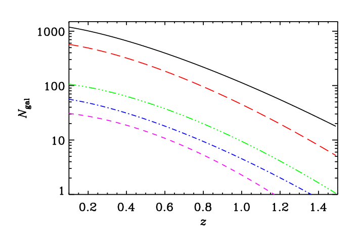
The final application of our simulations is to derive a relationship between the total cluster mass (or luminosity) and the number of recovered cluster galaxies. As Fig. 12 shows, the number of galaxies found by FOF is much more consistent and better-behaved than the number of galaxies detected by VT. Therefore we only use the FOF output to determine the total cluster mass. This is done by taking all galaxies that occur in the cluster in of the MC-realisations in which the cluster itself is detected. The galaxies that appear in a smaller fraction of MC-realisations are very likely to be interlopers from different redshifts. Calculating for all cluster-masses at all redshifts yields functions of vs. for total constant mass or luminosity. These are shown in Fig. 17. The number of detected galaxies at constant mass declines more steeply than a magnitude selected sample would, since the fraction of recovered versus simulated galaxies for the FOF method becomes smaller at higher redshift (see Fig. 12). The total cluster mass of cluster candidates found in real data (see VB06) can be estimated by overplotting the number of cluster galaxies and interpolating between the lines of constant cluster mass.
4 Summary
To summarise, the main points of this paper are set out below.
We have created a new cluster detection algorithm of which the main characteristics are: (i) each galaxy’s full redshift probability function is utilised, and (ii) cluster candidates are selected by cross-checking the results of two substantially different selection techniques: Voronoi Tessellations and Friends-Of-Friends.
Each selection technique is dependent on two parameters. Voronoi Tessellations uses , the limiting cell density, and , the maximum expected number of groups caused by background fluctuations. The parameters of the Friends-Of-Friends algorithm are , the linking distance, and , the minimum number of galaxies in a group.
Simulations using mock background galaxy catalogues with clusters superimposed allow us to choose optimum values for the algorithm’s parameters. We use , , , and .
Neither selection method shows an obvious bias to cluster ellipticity. However, the recovered shape of the clusters differs for both methods: VT tends to pick up more background galaxies at the edges of the clusters; by contrast, the galaxy members recovered by FOF are more centrally concentrated.
Cross-checking the output of the Voronoi Tessellations and the Friends-Of-Friends method eliminates spurious sources in the simulated cluster searches. However, low-level clustering within the background has not been taken into account.
Acknowledgments
The authors acknowledge STFC for financial support. Furthermore, we thank Steve Rawlings for useful discussions, Dave Bonfield for his efforts concerning the photometric redshift method, and all our co-authors on Van Breukelen et al. (2006). Finally, we are grateful to the referee for their helpful comments and suggestions to improve this paper.
References
Abell G. O. 1958, ApJS, 3, 211
Abell G. O., Corwin H. G. & Olowin R. P.,1989, ApJS, 70, 1
Bartelmann M., 1996, A&A, 313, 697
Bolzonella M., Miralles J.-M., Pelló R., 2000, A&A, 363, 476
Botzler C. S., Snigula J., Bender R., Hopp U., 2004, MNRAS, 349, 425
Bruzual G., Charlot S., 2003, MNRAS, 344, 1000
Cole S. et al., 2001, MNRAS, 326, 255
Delaunay B., 1934, Izvestia Akademii Nauk SSSR, Otdelenie Matematicheskikh i Estestvennykh Nauk, 7, 793
Dolag K., Bartelmann M., Perrotta F., Baccigalupi C., Moscardini L., Meneghetti M., Tormen G., 2004, A&A, 416, 853
Ebeling H. & Wiedenmann G., 1993, PhRvE, 47, 704
Gardner J. P., Sharples R. M., Carrasco B. E., Frenk C. S., 1996, MNRAS, 282L, 1
Gladders M. D. & Yee H. K. C., 2000, AJ, 120, 2148
Gladders M. D. & Yee H. K. C., 2005, ApJS, 157, 1
Goto et al., 2002, AJ, 123, 1807
Icke V., van de Weygaert R., 1987, A&A, 184, 16
Kiang T., 1966, Zeitschrift für Astrophysik, 64, 433
Kim R. S. J. et al., 2002, AJ, 123, 20
Koester B. P. et al., 2007(a), ApJ, 660, 221
Koester B. P. et al., 2007(b), ApJ, 660, 239
Lee D. T., Schachter B. J., 1980, Int. J. of Computer and Information Sci., 9, 219
Lin Y.-T., Mohr J. J., Stanford S. A., 2004, ApJ, 610, 745
Lobo C., Iovino A., Lazzati D., Chincarini G., 2000, A&A, 360, 896
Lopes P. A. A., deCarvalho R. R., Gal R. R., Djorgovski S. G., Odewahn S. C., Mahabal A. A., Brunner R. J., 2004, AJ, 128, 1017
Lucey J. R., 1983, MNRAS, 204, 33
Miller C. J., Nichol R. C., Gómez P. L., Hopkins A. H., Bernardi M., 2005, AJ, 130, 968
Navarro J., Frenk C., White S., 1997, ApJ, 490, 493
Postman M., Lubin L. M., Gunn J. E., Oke J. B., Hoessel J. G., Schneider D. P., Christensen J. A., 1996, AJ, 111, 615
Ramella M., Boschin W., Fadda D., Nonino M., 2001, A&A, 368, 776
Ramella M., Geller M. J., Pisani A., da Costa L. N, 2002, AJ,123, 2976
Rines K., Geller M. J., Kurtz M. J., Diaferio A., Jarrett T. H., Huchra J. P., 2001, ApJ, 561, L41
Sutherland W., 1988, MNRAS, 234, 159
Tucker D. L. et al., 2000, ApJS, 130, 237
Van Breukelen C. et al., 2006, MNRAS, 373L, 26
Van Breukelen C. et al., 2009, MNRAS, submitted
Van Haarlem M. P., Frenk C. S., White S. D. M., 1997, MNRAS, 287, 817