Magnetic properties of a spin-3 Chromium condensate
Abstract
We study the ground state properties of a spin-3 Cr condensate subject to an external magnetic field by numerically solving the Gross-Piteavskii equations. We show that the widely adopted single-mode approximation is invalid under a finite magnetic field. In particular, a phase separation like behavior may be induced by the magnetic field. We also point out the possible origin of the phase separation phenomenon.
pacs
03.75.Mn, 03.75.HhI Introduction
Since the realization of Bose-Einstein condensate of chromium atoms [1], there have been considerable experimental and theoretical efforts in exploring physical properties of chromium condensates. Owing to the large magnetic dipole moment of chromium atoms, the dipolar effects was first identified experimentally from its expansion dynamics [2]. More remarkably, with the precise control of the short-range interaction using Feshbach resonance, the -wave collapse of a pure dipolar condensate has been observed [3].
In the context of spinor condensates, chromium atom has an electronic spin , which provides an ideal platform for exploring even richer quantum phases as compared to those offered by the spin-1 and spin-2 atoms [6, 7, 8, 10, 9, 4, 5, 11, 12, 13]. To date, theorists have mapped out the detailed phase diagram of a spin-3 chromium condensate [15, 14, 16]. In particular, a more exotic biaxial nematic phase was also predicted [14]. The possible quantum phases and defects of spin-3 condensates were also classified based on the symmetry considerations [17, 18]. Other work on spin-3 chromium condensates includes theoretically studying the strongly correlated states of spin-3 bosons in optical lattices [19] and the Einstein-de Haas effect in chromium condensates [15, 20].
Nevertheless, all the previous work concerning the ground state and the magnetic properties of spin-3 Cr condensates has adopted the so-called single-mode approximation (SMA), which assumes that all spin components share a common density profile. However, the studies on spin-1 case show that, for an antiferromagnetic spinor condensate, SMA is invalid in the presence of magnetic field for antiferromagnetic spin exchange interaction [21]. One would naturally question the validity of SMA for spin-3 condensate since the short-range interactions involved here are more complicated than those in spin-1 system.
In the present paper, we study the ground state properties of a spin-3 chromium condensate subject to a uniform axial magnetic field by numerically solving the Gross-Pitaevskii equations. We show that even though SMA is still valid in the absence of an external magnetic field, it fails when the magnetic field is switched on. More remarkably, we find that when the undetermined scattering length corresponding to total spin zero channel falls into a certain region, the magnetic field may induce a phase separation like behavior such that the peak densities of certain spin components do not occur at the center of the trapping potential.
II Formulation
We consider a condensate of spin chromium atoms subject to a uniform magnetic field . In mean-field treatment, the system is described by the condensate wave functions (). The total energy functional of the system, , can be decomposed into two parts with and being, respectively, the single-body and interaction energies. Adopting the summation convention over repeated indices, the single-body energy can be expressed as
where is the mass of the atom, the trapping potential is assumed to be axially symmetric with being the trap aspect ratio, are the spin-3 matrices, is the Landé -factor of 52Cr atoms, and is Bohr magneton.

The collisional interaction between two spin-3 atoms takes the form [6, 7]
| (2) |
where projects onto the state with total spin and with being the scattering lengths for the combined symmetric channel . For 52Cr, it was determined experimentally that , , and with being Bohr radius [2], while the value of is unknown, and we shall treat it as a free parameter in the results presented below. Making use of the relations [6]
we may replace , , and in Eq. (2) by , , and , such that the interaction energy functional becomes
| (3) |
where the interaction parameters are , , , and . Furthermore, is the total density,
is the singlet amplitude, and
is the density of spin. Finally,
is the nematic tensor, and to obtain it, we have utilized the relation
The nematic tensor was first introduced in the liquid crystal physics as the order parameter [22] to describe the orientation order of the liquid crystal molecules. Since is Hermitian, it can be diagonalized with all eigenvalues (ordered as ) being real and the corresponding principle axes being mutually orthogonal. Unless all three eigenvalues are equal, the systems with two identical eigenvalues are usually refer to as uniaxial nematics, while those with three unequal eigenvalues are biaxial ones. More importantly, can be determined by performing Stern-Gerlach experiments along [14]. As it can be seen from Eq. (3), different quantum phases originate from the competition of , , and . Following the discussion of Diener and Ho [14], we shall characterize phases in a spin-3 Cr condensate using the condensate wave functions , singlet amplitude , spin , and nematic tensor .

To simplify the numerical calculations, we shall focus on highly oblate trap geometries () such that the condensate can be regarded as quasi-two-dimensional whose motion along the -axis is frozen to the ground state of the axial harmonic oscillator. The condensate wave functions can then be decomposed into
| (4) |
with and being normalized to the total number of atoms , i.e., . After integrating out the variable, gives an extra constant, while the interaction parameters , , , and are all rescaled by a factor . The mean-field wave functions are obtained by minimizing the total energy functional numerically using imaginary time evolution. We shall focus our study on the Cr line [14], namely only the scattering length is allowed to changed freely, since experimentally, it is the most relevant case. For all results presented in the present work, we have chosen , , and . Correspondingly, the dimensionless length unit is adopted in throughout this paper.
We remark that we have neglected the magnetic dipole-dipole interaction energy in Eq. (3) for simplicity, as in the present work, we are concentrating on investigating how short-range interaction and magnetic field affect the ground state wave function. The ignorance of dipolar interaction in spinor Cr condensate was also justified in Ref. [14]. Moreover, we have numerically confirmed that for the parameter used in this paper, the dipole-dipole interaction energy is much smaller than short-ranged spin-dependent interaction energy when the condensate is not polarized by the magnetic field.
III Results
Figure 1 summarizes the main results of this paper. In the left panel of Fig. 1, we present the phase diagram of spin-3 Cr condensate in the - parameter space, here we have adopted the similar notations for different phases as in Ref. [14]. In the right panel, we tabulate the major characters of each phase. We remark that the resolution of phase diagram is limited by step sizes of and when we numerically scan the parameter plane, therefore, it is possible that more details may emerge by reducing the step sizes.
III.1 Condensate wave functions
The numerical results indicate that the condensate wave functions can always be expressed as
| (5) |
where the density of th component is an axially symmetric function and the corresponding phase is a constant independent of the spatial coordinates. In case the external magnetic field is completely switched off, we find that all wave functions have the same density profile, indicating that the SMA is valid for spin-3 condensates in the absence of magnetic field. We note that this conclusion also holds true for spin- and - condensates.
Once the external magnetic field is applied, SMA quickly becomes invalid. More remarkably, as shown in Fig. 2, when control parameters and fall into the shaded region in the left panel of Fig. 1, the peak densities of at least one of the spin components among , , and do not occur at the center of the trap, in analogy to the phase separation in a two-component condensate [23, 24]. In the absence of magnetic field, the system is symmetric under SO(3) rotation of the spin, and component can be populated. However, immediately after we switch on the magnetic field, this SO(3) symmetry is broken such that spin components are highly populated under a very weak magnetic field. As one continuously increases the magnetic field, the occupation number in component increases with density in the margin of the trap growing faster than that in the center, which induces the phase separation like behavior. When the population in component dominates, the peak densities of all spin component occur at the center of the trap. We remark that similar behavior of the wave functions also appears outside the Cr line [14].

To gain more insight into the origin of the phase separation like behavior, we consider a homogeneous Cr condensate where each spin component has already condensed into the zero momentum mode. The wave function for phase unseparated state is then replaced by a uniform -number
| (6) |
where is a real constant and are complex constants. The ground state can be obtained by minimizing the total energy subject to the normalization condition . In such a way, we have reproduce the phase diagram in Ref. [14]. To confirm that those phases are indeed the ground states, we introduce a new set of variables, and , corresponding to, respectively, the real and imaginary parts of the wave function as
We then construct the Hessian matrix . For a solution to be stable, the Hessian matrix must be positive definite [25]. In Fig. 3, we present the unstable region of a homogeneous Cr condensate on - plane. To obtain it, we have chosen the density to be which is the peak density of the trapped system in our numerical calculations. One immediately sees that the unstable region of a homogeneous condensate roughly agrees with the phase separation region of the trapped system, which suggests that the possible origin of the phase separation behavior is the instability of the phase unseparated solution.
We emphasize that, unlike in a binary Bose-Einstein condensate where the emergence of phase separation is determined by the strengths of intra- and inter-species interactions, here for a given scattering length , the phase separation like behavior is induced by the magnetic field.
III.2 Singlet amplitude
Since the spatial independence of is a necessary condition for SMA, it can also be used as a criterion to check the validity of SMA. As shown in Fig. 4, is a constant when ; while immediately after the magnetic field is turned on, becomes spatially dependent. In addition, the peak value of decreases continuously as one increases the magnetic field until it completely vanish.
In Fig. 4 (a), becomes zero only after the condensate is completely polarized, while in (b) and (c), it vanishes once the system enters the phase. Therefore, using singlet amplitude, we may map out the phase boundaries between and , and , and and . However, alone is incapable of determining other phase boundaries. Finally, we note that, for , the value of drops much faster with the increasing magnetic field than that corresponding to , as shown below this behavior has a direct impact on the magnetization curve of the system.


III.3 Magnetization
We now turn to study magnetic field dependence of the total magnetization. To this end, we define the reduced magnetization as
| (7) |
Unlike in Ref. [16] where the total magnetization is conserved, here we allow it to change freely. Therefore, the transverse components of the spin, and , are always zero. Figure 5 shows the field dependence of the reduced magnetization, which approaches when reaches the saturation field. We note that, for , the behavior of slightly depends on the value of ; while for , the magnetization curves corresponding to different ’s become indistinguishable. Consequently, as shown in Fig. 1, the saturation field for the former case is a decreasing function of , while for the latter one, it becomes a constant. The independence of the magnetization for case can be qualitatively understood as follows. The scattering length only contributes to the total energy through singlet amplitude . As shown in Fig. 4, for , vanishes quickly as one increases the magnetic field, such that varying only yields a negligible effect on magnetization curve. With the help magnetization, we can further identify the phase boundary between and phases.
III.4 Nematic tensor
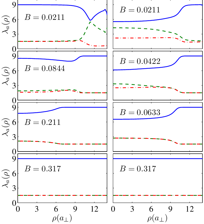
To determine other phase boundaries, we have to rely on the nematic tensor. In Fig. 6, we plot typical behavior of the eigenvalues of nematic tensor under different and magnetic fields. As a consequence of the failure of SMA, ’s are generally spatially dependent. However, some of their characteristics obtained under SMA remain to be true.
The full ferromagnet (FF) phase occurs when the magnetic field exceeds the saturation field such that only component is occupied. The nematic tensor takes a diagonal form with and . For the wave functions of A1 and H1 phases, only two spin states are populated: other than a common state, and are also occupied for, respectively, A1 and H1 phases. One can easily deduce that the nematic tensors of phases A1 and H1 are, respectively, and . Since for both cases, is the largest eigenvalue, we have . Moreover, and are spatially independent.
For G1 phase, and states are unoccupied, consequently, becomes a block diagonal matrix with one of the eigenvalues being . Furthermore, from numerical results, we find that is always the smaller eigenvalue and , which suggests that G1 is a biaxial nematic phase with .
All spin components of and phases are populated, they are all are biaxial nematic with three unequal and spatially dependent ’s. The principal axes for these phases are also spatially dependents. The only difference is that for phase we can identify that either or is perpendicular to -axis.
IV Conclusions
To conclude, we have mapped out the phase diagram of a spin-3 Cr condensate subject to an external magnetic field based on the numerical calculation of the ground state wave function. In particular, we show that SMA becomes invalid for Cr condensates under a finite magnetic field. More remarkably, if the unknown scattering length falls into the region , a phase separation like behavior may be induced by the magnetic field. We also point out that such behavior might originate from the instability of a phase unseparated solution. As a future work, we shall investigate the ground state structure of a spin-3 Cr condensate by including the magnetic dipole-dipole interaction.
Acknowledgements.
We thank Han Pu for useful discussion. This work is supported by NSFC (Grant No. 10674141), National 973 program (Grant No. 2006CB921205), and the “Bairen” program of the Chinese Academy of Sciences.References
- [1] A. Griesmaier, J. Werner, S. Hensler, J. Stuhler, and T. Pfau, Phys. Rev. Lett. 94, 160401 (2005).
- [2] J. Stuhler, A. Griesmaier, T. Koch, M. Fattori, T. Pfau, S. Giovanazzi, P. Pedri, and L. Santos, Phys. Rev. Lett. 95, 150406 (2005).
- [3] T. Lahaye, J. Metz, B. Fröhlich, T. Koch, M. Meister, A. Griesmaier, T. Pfau, H. Saito, Y. Kawaguchi and M. Ueda, Phys. Rev. Lett. 101, 080401 (2008).
- [4] J. Stenger, S. Inouye, D. M. Stamper-Kurn, H.-J. Miesner, A. P. Chikkatur, and W. Ketterle, Nature (London) 396, 345 (1998)
- [5] M. Barrett, J. Sauer, and M. S. Chapman, Phys. Rev. Lett. 87, 010404 (2001).
- [6] T.-L. Ho, Phys. Rev. Lett. 81, 742 (1998).
- [7] T. Ohmi and K. Machida, J. Phys. Soc. Jpn. 67, 1822 (1998).
- [8] C. K. Law, H. Pu, and N. P. Bigelow, Phys. Rev. Lett. 81, 5257 (1998).
- [9] M. Koashi and M. Ueda, Phys. Rev. Lett. 84, 1066 (2000).
- [10] C. V. Ciobanu, S.-K. Yip, and T.-L. Ho, Phys. Rev. A, 61, 033607 (2000).
- [11] H. Schmaljohann, M. Erhard, J. Kronjäger, M. Kottke, S. van Staa, L. Cacciapuoti, J. J. Arlt, K. Bongs, and K. Sengstock, Phys. Rev. Lett. 92, 040402 (2004).
- [12] M.-S. Chang, C. D. Hamley, M. D. Barrett, J. A. Sauer, K. M. Fortier, W. Zhang, L. You, and M. S. Chapman, Phys. Rev. Lett. 92, 140403 (2004).
- [13] T. Kuwamoto, K. Araki, T. Eno, and T. Hirano, Phys. Rev. A 69, 063604 (2004).
- [14] R. B. Diener and T.-L. Ho, Phys. Rev. Lett. 96, 190405 (2006).
- [15] L. Santos and T. Pfau, Phys. Rev. Lett. 96, 190404 (2006).
- [16] H. Mäkelä and K.-A. Suominen, Phys. Rev. A. 75, 033610 (2007).
- [17] R. Barnett, A. Turner, and E. Demler, Phys. Rev. Lett. 97, 180412 (2006); ibid. Phys. Rev. A 76, 013605 (2007).
- [18] S.-K. Yip, Phys. Rev. A 75, 023625 (2007).
- [19] J.-S. Bernier, K. Sengupta, and Y.-B. Kim, Phys. Rev. B 76, 014502 (2007).
- [20] Y. Kawaguchi, H. Saito, and M. Ueda, Phys. Rev. Lett. 96, 080405 (2006).
- [21] S. Yi, Ö. E. Müstecaplıoğlu, C. P. Sun, and L. You, Phys. Rev. A 66, 011601(R) (2002);
- [22] P. G. de Gennes and J. Prost, The Physics of Liquid Crystals, 2nd ed (Oxford University Press, London, 1993).
- [23] C. J. Myatt, E. A. Burt, R. W. Ghrist, E. A. Cornell, and C. E. Wieman, Phys. Rev. Lett. 78, 586 (1997); D. S. Hall, M. R. Matthews, J. R. Ensher, C. E. Wieman, and E. A. Cornell, Phys. Rev. Lett. 81, 1539 (1998).
- [24] T. L. Ho and V. B. Shenoy, Phys. Rev. Lett. 77, 3276 (1996); H. Pu and N. P. Bigelow, Phys. Rev. Lett. 80, 1130 (1998).
- [25] E. Timmermans, Phys. Rev. Lett. 81, 5718 (1998)