Measuring the galaxy-mass and galaxy-dust correlations through magnification and reddening
Abstract
We present a simultaneous detection of gravitational magnification and dust reddening effects due to galactic halos and large-scale structure. The measurement is based on correlating the brightness of 85,000 quasars at with the position of 20 million galaxies at derived from the Sloan Digital Sky Survey and is used to constrain the galaxy-mass and galaxy-dust correlation functions up to cosmological scales.
The presence of dust is detected from 20 kpc to several Mpc, and we find its projected density to follow: , a distribution similar to mass. The amount of dust in galactic halos is found to be comparable to that in disks. On large scales its wavelength dependence is described by , consistent with interstellar dust. We estimate the resulting opacity of the Universe as a function of redshift and find mag up to . This, in turn, implies a cosmic dust density of , roughly half of which comes from dust in halos of galaxies.
We present magnification measurements, corrected for dust extinction, from which the galaxy-mass correlation function is inferred. The mean mass profile around galaxies is found to be up to a radius of 10 Mpc, in agreement with gravitational shear estimates.
Keywords:
dust – extinction, reddening – dark matter – magnification – large-scale structures – quasars – galaxies1 INTRODUCTION
Light rays from distant sources carry unique information about the matter and gravitational potential along the line-of-sight. A well-known example is the signature of intervening gas clouds imprinted into spectra of background sources via absorption lines. Mass concentrations located along the path of photons can also induce gravitational lensing effects. Background sources can be magnified, as detected by Scranton et al. (2005), and galaxy shapes can be distorted as measured through galaxy-galaxy lensing (cf. Hoekstra et al. 2002, Sheldon et al. 2004, Mandelbaum et al. 2005, Leauthaud et al. 2007; Parker et al. 2007) and cosmic shear (e.g. Fu et al. 2008). Measuring these effects has become a powerful tool for probing the mass distribution in the Universe.
In addition, dust extinction effects are expected to occur as radiation pressure from stars and galactic winds triggered by supernovae are expected to expel some amount of dust from galactic disks into the intergalactic medium (Aguirre, 1999; Bianchi & Ferrara, 2005). Detecting dust reddening by galaxy halos would provide us with useful information on the life cycles of dust particles as well as characterize the opacity of the Universe. In practice, detecting such an effect is made difficult by the requirement to measure brightness and/or color changes at a sub-percent level on 100 kpc scales around galaxies. A first attempt to find dust in galactic halos was made by Zaritsky (1994) who reported a 3- indication for a color change of background galaxies found around two nearby spiral galaxies. Probing dust reddening induced by galaxy halos has not been revisited since then, despite the dramatic improvement in data quality and sample size.
In this work we investigate simultaneously gravitational lensing and
dust reddening of background quasars by foreground
galaxies and associated large scale structure.
Our observational results primarily make use of the angular
cross-correlation between the brightness of quasars and the projected
density of galaxies. We first recover and improve upon previous
measurements of the magnification of quasar images by gravitational
lensing due to galaxies located nearby the light paths using a sample
of 85,000 quasars behind 20 million galaxies derived from the Sloan
Digital Sky Survey (York et al. 2000; SDSS) Data Release 3
(Abazajian et al. 2005). Second, this large sample – together with high
accuracy photometry in five optical pass bands – allows us to detect
the presence of dust in the intervening space and explore its
distribution and properties. This allows us to study the properties
of intergalactic dust and provides a way of inferring the abundance of
dust in the Universe.
We introduce the formalism of brightness-density correlations in §2. Data processing and measurements are presented in §3 & §4. The astrophysical results are given in §5 and we summarize in §6. When needed we use , and .
2 Formalism of Brightness-Density correlations
Let us begin by considering a background source angularly close to a foreground galaxy. This galaxy acts as a gravitational lens, magnifying the source flux and giving rise to extinction and reddening due to the presence of dust surrounding it. The observed flux is then modified by the combination of these effects according to
| (1) |
where is the gravitational magnification and is the optical depth for dust extinction at an observed wavelength . The corresponding magnitude shift is
When departs weakly from unity, we can re-express this relation as
| (2) |
where . Thus, magnification and extinction compete in changing the brightness of background sources. Dust extinction is in general wavelength dependent while magnification is achromatic, so the two effects can, in principle, be separated using multi-color data. Below we show how correlations between the density of foreground galaxies and the magnitude of background sources allow us to constrain the galaxy-mas and galaxy-dust correlation functions.
2.1 The galaxy-mass correlation probed with magnification
The galaxy-mass correlation is a powerful tool to probe the connection between matter and galaxies, providing direct constraints on the dark matter distribution and models of galaxy formation. To introduce it, we first define the galaxy and mass overdensities:
| (3) |
where and are the density of galaxies and matter. The galaxy-mass correlation is then defined by
| (4) |
This cross-correlation can be related to the projected surface density of galaxies:
| (5) | |||||
The first relation indicates that the galaxy-mass correlation is equal to the mean mass profile around galaxies, at a given separation . The second relation is simply a projection of the 3-dimentional galaxy-mass correlation introduced above in Equation 4 and where .
The mass surface density can be probed with gravitational lensing. In the weak lensing regime, it is straightforwardly related to the observable magnification, according to
| (6) |
Here is the lensing convergence and the critical mass surface density is given by
| (7) |
where and are respectively the angular diameter distances to the lens, the source and between the lens and the source.
As indicated in Equation 2, magnification will affect the brightness of background sources and induce a correlation between the density of foreground galaxies and the magnitude of background sources. In order to understand the impact on observable quantities, let us consider a given area of the sky and let be the intrinsic magnitude distribution of some sources. The photons originating from these sources may be deflected by gravitational lensing and magnification affects their magnitude distribution such that
| (8) |
where is the induced magnitude shift. This leads to an observable mean magnitude shift:
| (9) |
It should be noted that for a magnitude-limited sample of sources, the mean magnitude shift induced by a population of foreground galaxies, , differs from the observable mean magnitude shift of the individual sources, . The difference between the two depends on the shape of the source magnitude distribution and the limiting magnitude of the sample. In the case where the induced magnitude shift is small compared to the limiting magnitude of the sample, the difference between the observed and induced magnitude shift can be linearized in and we have
| (10) |
where the coefficient depends on the shape of the magnitude distribution and the limiting magnitude. In the considered limit, it is given by
| (11) |
(see the derivation in the appendix). If the sample of sources is not
magnitude-limited, and ,
i.e. the measured magnitude shift equals the induced one. For
magnitude-limited samples, in general we have , i.e. the
observable magnitude shift is smaller than the induced one. It is
important to note that for power-law luminosity distributions . Therefore, while the brightness of each object changes by
, the mean magnitude of the sample remains unchanged. This
is due to the inclusion of sources which become brighter than the
limiting magnitude. For SDSS quasars in the -band, down to a
limiting magnitude of , we find .
Let us suppose that a population of background quasars and foreground galaxies are sufficiently well separated in redshift so that physical correlations between them can be neglected. Gravitational lensing will give rise to an apparent correlation between quasar brightness and the proximity to a galaxy overdensity, which we can write as
| (12) | |||||
where is the quasar magnitude fluctuation and is the foreground galaxy overdensity at a given angular distance from a background source. If magnification effects are in the weak regime, i.e. , the above relation reads
| (13) | |||||
On scales below a few arcminutes, a non-linear treatment of the magnification as a function of the density contrast is needed. Such calculations are presented in Ménard et al. (2003), where the authors show that non-linear effects can increase the amplitude of the magnification by about 30% at a scale of one arcminute.
For populations of quasars and galaxies selected over an appreciable redshift range, the above correlation can be expressed in terms of the galaxy-dark matter cross-power spectrum using the Limbers’ approximation. Following the formalism introduced by Bartelmann (1995) and the notation laid out in Jain, Scranton & Sheth (2003), we can write
| (14) | |||||
where is the cosmological matter density relative to
critical, is the comoving distance, is the lensing
kernel, and is the galaxy-dark matter cross-power
spectrum. The quantity therefore probes the magnification due to individual
galaxy halos on small scales and on large
scales it constrains the large scale distribution of matter in the Universe.
2.2 Dust extinction and reddening
Statistical properties of the distribution of dust around galaxies can be constrained by the galaxy-dust correlation function:
| (15) |
where is the dust density fluctuation. This cross-correlation can be related to the projected dust surface density of galaxies:
| (16) | |||||
At optical wavelengths, dust extinguishes and reddens the light of background sources. The galaxy-dust correlation can then be probed by measuring the cross-correlation between the colors of background sources and the distribution of foreground matter.
Let us define the magnitude shift of a background source measured at a wavelength with respect to the mean magnitude of the sample,
| (17) |
Expanding the formalism introduced in the previous section to dust reddening effects, and defining the color excess
| (18) | |||||
we introduce the quasar color-galaxy density correlation, which can be used to probe the galaxy-dust correlation:
| (19) |
If the foreground galaxy and background source populations are well separated in redshift, the above correlation provides us with information on the mean reddening and therefore the mean amount dust around galaxies. The information at different wavelengths can be used to probe the shape of the extinction curve. For scales on the order of a typical galaxy virial radius and smaller, the signal is expected to be dominated by single galaxies and provides with the average dust density profile around galaxies. On larger scales it provides information as to the large scale distribution of dust in the Universe.
For a given extinction curve the above quantity can be used to infer the mean dust extinction profile around galaxies , or similarly the mean optical depth for dust extinction .
It should be noted that not only extinction but also reddening effects
can cause quasars to drop out of the selection criteria as their
identification is a function of colors. In the latter case, the
measured reddening excess turns out to be lower than the true value
and the relation between observed and induced color change needs to be
quantified. In the present analysis, reddening effects are
sufficiently small for this to be negligible (see discussion below).
3 ANALYSIS
3.1 The data
The data set consists of galaxy and quasar catalogues and is drawn from the third SDSS data release (DR3; aba03). The survey provides images in five broad optical bands ( Fukugita et al. 1996; Smith et al. 2002). Before masking, this set covers roughly 5300 square degrees, the majority of which is located around the North Galactic Cap. To reduce systematic errors in the photometric data, we impose a seeing limit of 1”4 and a Galactic extinction limit of 0.2 in the band (Scranton et al. 2002). We also apply a mask blocking a one-arcminute radius around bright galaxies () and stars with saturated centers to prevent changes in the source number densities due to local fluctuations induced by errors in sky brightness subtraction (Mandelbaum et al. 2005). Altogether, the masks reduce our total area to square degrees.
With these cuts, we can reliably perform star/galaxy separation using Bayesian methods to (Scranton et al. 2002), yielding a galaxy sample whose density is independent of local variations in seeing, Galactic extinction, sky brightness or stellar density after masking. This yields about 24 million galaxies between at a density of approximately 1.8 galaxies per square arcminute. The Scranton et al. (2005) paper used a sample that was instead r-band limited, which accounts for the difference in the galaxy sample sizes.
For galaxy magnitudes, we use composite model magnitudes, constructed from the expMag, devMag and fracDev parameters in the SDSS database. This provides a more robust estimate of galaxy flux at faint magnitudes than the Petrosian magnitudes used in the SDSS spectroscopic sample, which can have strong variations due to local seeing for . For quasars, we consider the flux within the psf profile, designated as psfMag. All magnitudes are de-reddened to correct for Galactic extinction before applying the various magnitude cuts.

The quasar data set was generated using the kernel density estimation (KDE) method described in Richards et al. (2004) applied to the DR3 data set. The KDE method is an extension of the traditional color selection technique for identifying quasars. Two training sets, one for stars and one for quasars are prepared and the colors for each object are compared to those of the two training sets using a 4D Euclidean distance. The objects are then classified as either quasar or star according to a larger probability of membership. This technique allows a clean separation of relatively low redshift () quasars from the stellar locus, producing a catalog of 225,000 quasars down to a limiting magnitude of with efficiency and completeness greater than the SDSS spectroscopic target selction algorithm (Richards et al. 2002; Blanton et al. 2003). After masking, the total quasar population is reduced to 195,000. 11 1 Upcoming analyses will make use of the larger and deeper SDSS photometric quasar catalog (Richards et al., 2007), increasing the number of objects by an appreciable amount.
In addition to finding quasars, we applied photometric redshift techniques (Weinstein et al. 2004) to exclude low redshift quasars which might be physically associated with our foreground sample. Quasar photometric redshifts are driven by the broad spectral emission features in their spectra, resulting in photometric redshift likelihoods that can have multiple peaks as well as strong asymmetries around the most likely redshift. Rather than estimating a Gaussian redshift error, we use an upper and lower redshift bounds for a specified likelihood. To minimize the overlap with the galaxies in the redshift space, we require the upper and lower bounds to be within the range . The corresponding distribution of quasar redshift probabilities is shown in Figure 1 with the red line. For simplicity we treat the redshift p.d.f. of each quasar as a flat distribution between the upper and lower redshift bounds described above and weighted by the likelihood that the redshift was within those bounds. This final selection criterion reduces the number of quasars to 85704.


We estimate the overall shape of the galaxy redshift distribution based on the CNOC2 luminosity functions (Lin et al. 1999) following the treatment described in Dodelson et al. (2002). This distribution is well fit by the expression
| (20) |
plotted with the solid blue curve. The mean redshift for the galaxy sample is found to be
| (21) |
For lensing purposes it is useful to compute the galaxy redshift distribution weighted by the expected lensing efficiency. We have computed this quantity using the quasar redshift distribution and we show it using the blue dashed line in the figure. The effective redshift weighted by the lensing efficiency is given by
| (22) |
It is found to be .
Figure 2 shows the quasar magnitude and color distributions. As can be seen, the quasar sample is magnitude limited in but not color limited. While quasars are selected both in magnitude and color space, the modes of the color distributions are far from the limiting colors. As a result, a measured color change can be directly used as an estimate of the intrinsic color change of the population. Such a property is not satisfied for magnitude changes (see section 2.2 for more details).

3.2 Measurement
We measure the density of galaxies (taking into account missing area due cuts on the local seeing variations, bright stars, etc.) and compute its correlation, , with the magnitude of background quasars in the band , as a function of angular separation:
| (23) |
On small scales (), the signal contributions from magnification and dust extinction are expected to be dominated by Poisson noise. For larger scales, measurements from different angular bins become significantly correlated, as one would expect since different quasars will be sampling the same local population of galaxies. Since we are looking for very small variations in the quasar magnitude and galaxy density, the photometric calibration across the survey needs to be highly homogeneous. To avoid possible drift in the SDSS calibration over time, we measure the QSO-brightness galaxy-overdensity correlation separately on each stripe of the survey, and then take the average over all stripe-based estimators 22 2 Adjacent stripes of SDSS data may be taken on nights with significant observational lag. As such, the photometric zero points across stripes are not always calibrated to the precision required for this measurement. In principle, this implies that we should only use data from single scans over one night. However, in practice, we find that stripe-by-stripe treatment yields a sufficent photometric zero point accuracy to avoid systematic effects on the angular scale of the SDSS stripe. In the future, using the photometric über-calibration (Padmanabhan et al., 2008) might solve some of the above issues. :
| (24) |
where is the QSO-magnitude galaxy-overdensity
correlation measured for stripe using the filter . The
associated cost is to reduce the sensitivity of the estimator to power
arising from one direction, i.e., the scanning direction, which is
equivalent to reducing the size of the sample when measuring the
large-scale power. Our strongest signal is on angular scales smaller
than the width of a single stripe () so the
extent of this effect should be minimal.
In order to measure reddening induced correlations, we compute the difference between two stripe-based estimators at different wavelengths,
| (25) |
To estimate the error on the above estimators we use bootstrap samples of the quasar catalog with which we re-measure the above quantities and estimate their dispersion.
4 RESULTS

Following the above procedure we measure the correlation between the observed QSO brightness excess and galaxy density (Equation 23), where denotes one of the five SDSS pass bands, with the errors estimated from bootstrap resampling. The results shown in Figure 3 are examples for the and bands. We observe that quasar magnitude shifts and galaxy overdensities are anticorrelated. In other words, quasars appear to be brighter when closer to galaxies, which implies a dominance of magnification over extinction effects for the main sample of SDSS galaxies with . At the same time, the systematically larger amplitude in the redder band indicates the presence of a wavelength-dependent effect which could be attributed to dust extinction.
Before interpreting these signals, we note that both magnification and reddening effects are observed over a wide range of scales, from about 5″to a few degrees. We have therefore expanded the angular range used in the detection of magnification by Scranton et al. (2005) to both smaller and larger separations. Using the mean galaxy redshift computed in Equation 21 an angular scale of one arcminute corresponds to roughly 150 kpc. The above angular range thus corresponds to physical scales from kpc to Mpc, as indicated in the top abscissa of the figure.
In the inset of Figure 3, we show the wavelength dependence of the signal on small-scale with measurements of with the and filters. We can observe a continuous trend as a function of wavelength: the signal is systematically stronger in redder bands, consistent with reddening by dust. This also shows that probing magnification requires a correction for the effects of dust extinction.
Systematics Tests
Based on the same quasar sample and a slightly brighter galaxy sample (selected with ) Scranton et al. (2005) used a density-based estimator and showed that the dominant magnification signal of the quasar-galaxy correlation follows the expected dependence as a function of quasar magnitude. No such behavior could be detected when using stars instead of quasars as a control sample.
The amplitude of dust reddening depends only on the properties and amount of dust around the foreground galaxies selected for the cross-correlation. We can recover a similar wavelength-dependent extinction as in Figure 3 or the mean reddening signal presented in Figure 4 by using subsamples of quasars in different magnitude ranges. As a further sanity check, we also replaced our quasars with stars selected to have the same magnitude and spatial distribution on the sky. Measuring the cross-correlation between star brightness and galaxy overdensity with this sample, we find no appreciable color excess for galaxies with and stars selected in various magnitude ranges.33 3 We have detected, however, some excess reddening for stars when fainter galaxies () are used. This effect is likely to be attributed to a small contamination of faint galaxies in the stellar sample at faint magnitudes where star-galaxy classification is incomplete. This is expected to occur at . The presence of galaxies in the star sample may give rise to a similar correlation between source reddening and galaxy overdensity, since galaxy clustering gives rise to an excess of redder galaxies in overdense regions, which produces a similar signal that mimics the reddening by dust. We have measured the reddening-clustering correlation of SDSS galaxies with and found that a contamination of galaxies at about 10% could explain the reddening signal seen around stars. Finally, we have investigated the dependence of the signal as a function of Galactic reddening: by splitting the dataset into two regimes of Galactic extinction given by the Schlegel et al. (1998) map, we did not detect any significant change in our signal.
4.1 Reddening
4.1.1 Scale dependence
We isolate the reddening effects by measuring the correlation between QSO color and foreground galaxy overdensity, , where and indicate two different pass bands. We estimate the errors by computing the color covariance matrix from bootstrap resampling. Note that the errors on colors are smaller than the errors on brightness changes. As Figure 4 shows, quasar colors and galaxy overdensities are positively correlated, i.e. quasars appear to be redder when closer to high concentrations of foreground galaxies. The reddening effects are detected for all color combinations, from to about , corresponding to physical scales ranging from 50 kpc to about 10 Mpc. The measurement probes galactic radii well beyond the size of galactic disks. The amplitude of the effect is stronger in bluer bands. We find that a background source whose light passes at around 20 kpc from a foreground galaxy (selected with ) will be, on average, redder by mag.
4.1.2 Wavelength dependence
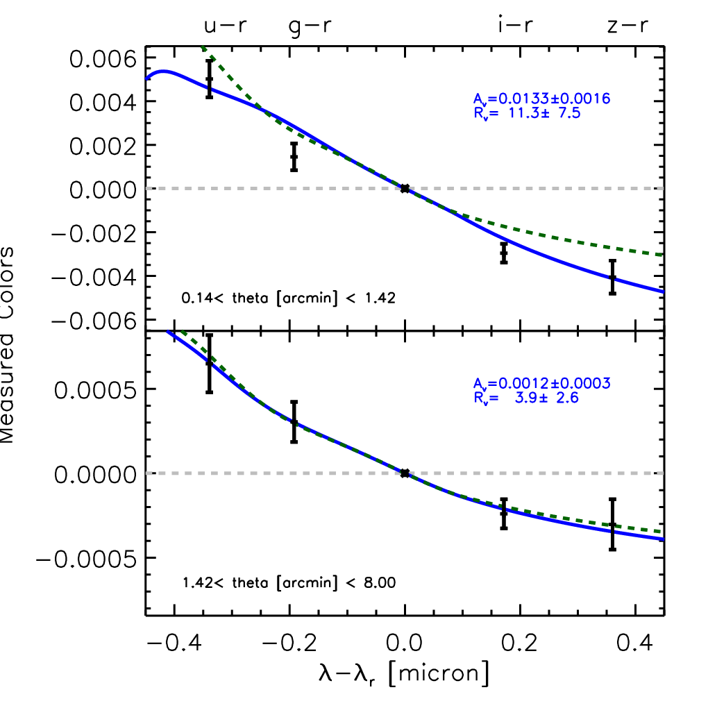
The five SDSS filters allow us to constrain the shape of , the extinction curve of the dust associated with the galaxies, through four independent colors. We measure the correlations for two angular bins: arcmin and arcmin, which correspond to effective projected radii of about kpc and Mpc. In Figure 5 we show the corresponding color excesses with respect to the band. We compare these reddening measurements to the standard extinction curve by fitting these data points with the functional form of the extinction curve provided by O’Donnell (1994). Such extinction curves are usually characterized by the parameter , which characterizes the slope of the extinction curve. The coefficient quantifies the amount of dust through its extinction in the band. The best fit for and is shown with the blue curve. On small scales our measured reddening corresponds to mag and , i.e. the slope of the extinction curve is not well constrained. On large scales however we obtain a better accuracy:
| (26) |
and mag. The green dashed curve shows the best fit for when is assumed to be 3.1, the standard value for dust in the disk of our Galaxy. Within the errors our results are consistent with standard interstellar dust.
4.2 Dust extinction
Given our measurements of the reddening due to foreground galaxies, we can now make estimates of the average dust extinction profile of the galaxies in our sample. In addition to constraining the amount and spatial distribution of dust on large scales around galaxies, this quantity is of interest to quantify the intrinsic brightness of background sources, which is the main goal of Type Ia supernovae measurements aimed at constraining dark energy.
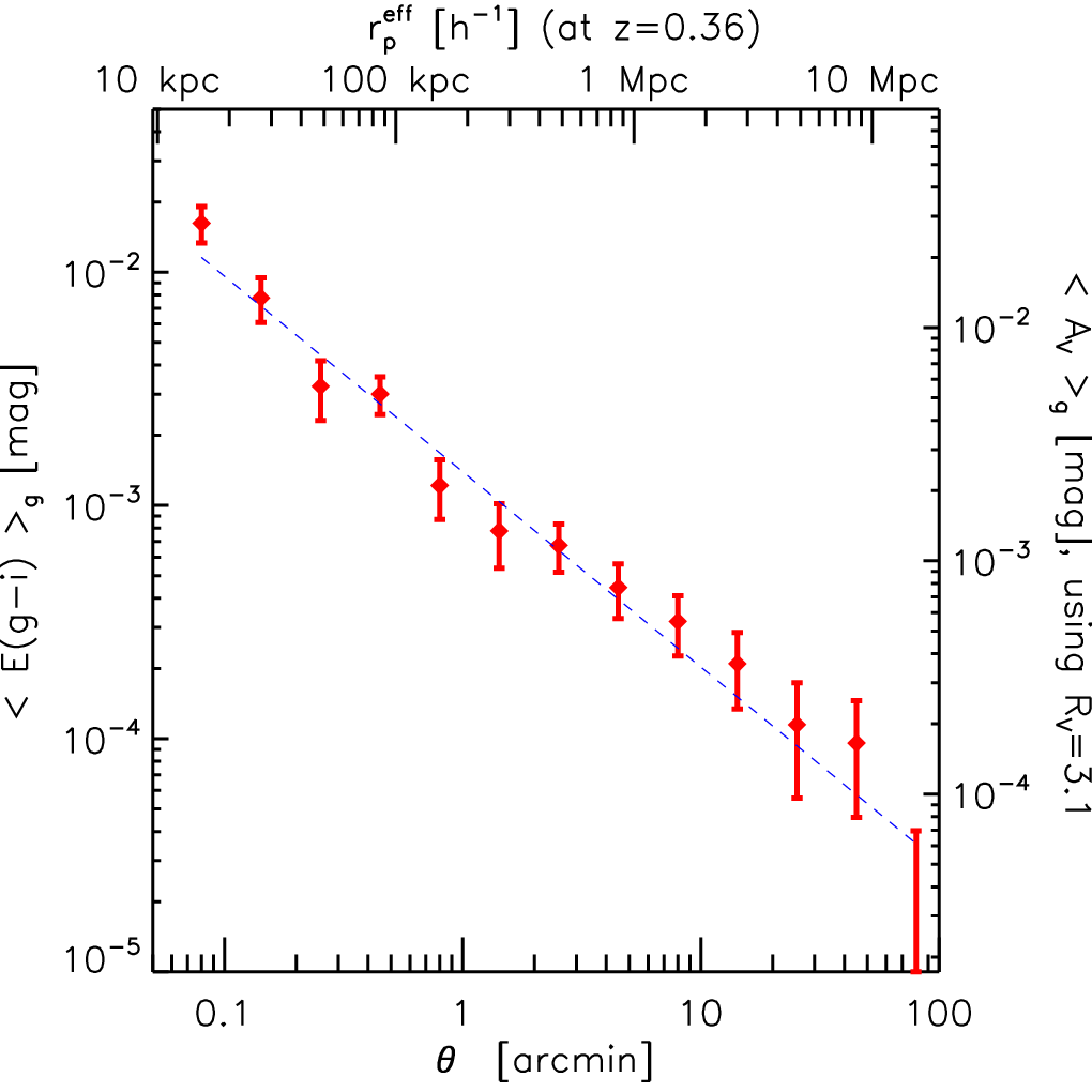
As indicated in §2.2, the correlation between quasar color and galaxy overdensity is an estimator of the mean reddening induced by galaxies. In order to maximize the signal-to-noise ratio of the reddening detection, we measure the quantity for which and are taken to be the and pass bands. We avoid using the and bands for which the photometric errors are substantially larger. In addition, the latter suffers from photometric contamination due to sky emission lines. We show the mean color excess of quasars as a function of scale in Figure 6. A best fit power-law gives
| (27) |
This quantity is proportional to the dust surface density and
therefore provides us with direct constraints on the spherically
average distribution of dust around galaxies. The angular dependence
is similar to average mass profiles around galaxies constrained from
galaxy-galaxy lensing
(e.g. Sheldon et al. (2004); Mandelbaum et
al. (2005)) and
magnification measurements by Scranton et
al. (2005).
This result has a number of implications regarding the amount and
nature of the dust in galaxy halos. It will be discussed below
in section 5.
In order to convert reddening into extinction, we choose the value , corresponding to standard interstellar dust in our Galactic disc and in agreement with the constraints obtained above. In Figure 6, we plot the mean extinction profile around the galaxies in our sample. It can be written as
| (28) |
or
| (29) |
where is the observed -band extinction. For an extinction curve characterized by , we have in the visible range. We point out that the amount of reddening profile shown in Figure 6 is significantly lower than contributions expected from dwarf galaxies. For example, the average dust reddening induced by the LMC, located at about 50 kpc from our Galaxy, is (Schlegel et al., 1998). Such a value is about an order of magnitude larger than eq. 27 and shows that satellite galaxies are expected to dominate the amount of dust reddening for individual lines-of-sight intercepting galaxy halos.
4.3 Magnification

The correlation between quasar magnitude shift and galaxy overdensity allows us to constrain a combination of magnification and dust extinction. Having estimated the wavelength-dependent extinction from reddening measurements in the previous section, we can now use this information and isolate the magnification effects. Our goal here is to estimate the signal well enough to allow for a comparison with similar measurements from galaxy-galaxy lensing available in the literature.
For simplicity we start by describing the angular correlation between quasar brightness and galaxy overdensity by a simple power-law with index . As above, we use a value of (or in the visible range) to convert reddening into extinction. The mean quasar brightness change as a function of angular separation from galaxies then reads
| (30) |
where is the achromatic magnitude change due to magnification and is the change due to dust extinction in the V-band. As shown above, we have (Eq. 28), which gives .
At sufficiently large wavelength, dust extinction becomes negligible and the brightness change is only due to magnification. In this limit, we find
| (31) |
where we have used the conversion between observed and induced
magnitude shift (Equation 13) and for
SDSS quasars with (Equation 11). This implies that the
mean magnification excess found at one arcminute (or 100 kpc) is
about 2%. This result is in agreement with that of
Scranton et
al. (2005) where the authors inferred the
magnification from the observed correlation between quasar and galaxy
densities on the sky, i.e. a different estimator. Our analysis also
allows us to measure magnification effects on smaller scales.
On the smallest scale we can probe, i.e. 5″(or 15 kpc),
we find .
In the weak lensing regime, the magnification is related to the mean mass surface density by
| (32) |
The inferred mean mass surface density of our galaxy sample is shown with the blue data points in Figure 7. A best fit power-law distribution gives
| (33) |
with , or using our effective projected scale:
| (34) |
with . These results provide an estimate of galaxy density profiles from gravitational magnification corrected for dust extinction effects. While a linear relation between magnification and density contrast is a good approximation on large scales, higher-order corrections become significant on scales smaller than a few arcminutes. As shown by Ménard et al. (2003), using Eq. 32 results in overestimating the projected mass by about 15 to 25% on scales ranging from 1 to 0.1 arcminute. The first few points shown in Figure 7 have not been corrected for this effect. As shown below, on larger scales the mass estimate from magnification is in good agreement with shear-based mass estimates.
4.3.1 Comparison with shear measurements
So far the galaxy-mass cross-correlation has mostly been accessible through galaxy-galaxy lensing measurements which estimate the mean tangential shear of background galaxies for a given sample of foreground lenses (e.g. Hoekstra et al. 2002, Sheldon et al. 2004, Mandelbaum et al. 2005, Leauthaud et al. 2007). The tangential shear () azimuthally averaged over a thin annulus at projected radius R from a lens galaxy is directly related to the projected surface mass density of the lens within the aperture,
| (35) |
where
| (36) |
is the mean surface density within radius , and is the azimuthally averaged surface density at radius (Miralda-Escude 1991; Fahlman et al. 1994). Therefore, shear measurements constrain whereas magnification is a direct estimate of .
In order to compare magnification and shear measurements, it is interesting to note that, in the case of power-law mass profiles, with , we have
| (37) |
The two observables and are therefore equivalent for isothermal profiles. For an angular dependence following , we have with . This value goes down to for an index of . Using galaxy-galaxy measurements based on the SDSS, Sheldon et al. (2004) found with and for a sample of spectroscopically identified lenses with and . Considering for simplicity a slope of (consistent with their constraint), their results translate into . Their scaled-measurements (using Equation 37) are shown in Figure 7. Under these assumptions, the magnification and shear estimators appear to be in very good agreement. A more accurate comparison between the two would require accounting for the differing luminosity distributions between the two lensing samples as well possible redshift evolution (our lenses comprising most of the sources for the shear-based estimators). However, it illustrates that both methods offer comparable degree of measurement precision and dynamic range while affected by significantly different systematic effects.
5 IMPLICATIONS
Our detection of the change in apparent magnitude of distant quasars has
allowed us to quantify the magnification and reddening of background sources
as their light rays pass in the vicinity of foreground galaxies.
While the amplitude of gravitational lensing effects has been known both
from theory (Bartelmann, 1995; Ménard
& Bartelmann, 2002; Jain, Scranton & Sheth, 2003)
and observations (Scranton et
al., 2005), the expected amplitude
of dust reddening and extinction effects was largely unconstrained.
Our study has shown that, in the visible bands, dust extinction occurs at a
level comparable to that of the observed brightening due to magnification.
Hence, studies aimed at predicting observable
magnitude changes of background sources (quasars, galaxies,
supernovae, etc.) which include only gravitational lensing effects are
incomplete. In the visible range, dust
extinction effects cannot be neglected and must be included alongside with
magnification to properly account for the effects of passing through
large scale structure.
Below, in order to simplify the discussion we will assume the dust in
galactic halos to be described by SMC type dust.
This choice is motivated by a number of results: (i) certain
low-ionisation absorbers such as MgII are known to inhabit the halo of
galaxies. They are found on scales reaching up to about
100 kpc around galaxies (Zibetti et
al., 2007). Recently several
authors studied their extinction properties and dust content
(Ménard et
al., 2005; Khare et al., 2005; York et al., 2006).
They found that their average extinction curve is similar to that of
the SMC, i.e. does not show the 0.2 bump seen in the Milky
way extinction curve (for systems with where the feature
enters the visible window). (ii) In addition, it is known that only
a small fraction of high redshift galaxies show an extinction
curve with the bump. As discussed below, considering a Milky-Way type dust changes our results only by a factor two.
In order to characterize the population of galaxies responsible for most of the intergalactic dust, we first assume that the amount of dust in halos is, on average, proportional to the metallicity and luminosity of galaxies. Under this assumption, the dominant contribution of the reddening signal is expected to originate from galaxies with an effective luminosity:
| (38) |
where is the galaxy luminosity density given by the Schechter function
| (39) |
with and is the metallicity-luminosity relation (Tremonti et al., 2004):
| (40) |
with . By integrating Equation 38 between and infinity, we find that the most important contribution of reddening originates from galaxies with a luminosity
| (41) |
Given the number density of galaxies (Fukugita & Peebles, 2006) and the above
luminosity function, galaxies with are expected to have a comoving number density of .
Below we discuss a number of implications given by the existence of a large-scale distribution of dust around galaxies. We note that only certain of the following results will make use of the above numbers.
5.1 Dust mass distributions
The properties of dust particles giving rise to the observed optical extinction and infrared emission in our Galaxy, the LMC and the SMC have been modeled by several authors (e.g. Mathis 2000 and Weingartner & Draine 2001). These models provide estimates of the absorption cross section per mass of dust as a function of wavelength , which is used to infer dust mass surface density from reddening profiles. For the SMC type dust the model of Weingartner & Draine (2001) gives 44 4 We thank Joseph Weingartner for having provided us with this value.
| (42) |
Note that Milky Way type dust corresponds to a dust mass larger by a factor two at a fixed extinction.
5.1.1 Evidence for a diffuse component of dust in galaxy halos
The knowledge of allows us to convert the observed reddening into a dust mass surface density. The spatial dependence of this quantity is shown in Figure 8. We find a column density of dust of about at an impact parameter of 100 kpc. It is interesting to estimate the total amount of dust in the halo of the galaxies defined by Equation 41. Considering an isothermal sphere mass distribution, the virial radius of galaxies is . The mass of dust residing in the halo of such galaxies is given by integrating the ratio over the area enclosed by :
| (43) |
Our measurements provide us with the radial dependence of for kpc, i.e. scales greater than galactic disks. By defining the dust mass in the halo as and using eq. 28 with SMC type dust, we find
| (44) |

This estimate shows that a substantial amount of dust exists in the halo of galaxies. This dust mass is comparable to that commonly found in galactic disks (Draine et al., 2007). This immediately shows that the reddening profile shown in Figure 6 cannot be explained by a contribution from satellite galaxies whose luminosities and therefore dust masses is negligible compared to a central galaxy. Our results suggest the existence of a diffuse component of dust in galactic halos.
We note that similar arguments can be obtained from reddening considerations and do not rely on the specific value of (Eq. 42). It should also be noted that while the total amount of dust appears to be dominated by a diffuse component, the largest reddening values are still expected to originate from lines of sight passing through satellites. The average reddening value of the LMC, , is about one order of magnitude larger than the average halo reddening at a radius on order 50 kpc (see Figure 6).
5.1.2 Dust-to-mass ratio
Having obtained constraints on both the total mass distribution from magnification and dust mass from reddening (see Figure 8), we can compare their statistical spatial distributions by computing the ratio
| (45) |
where and are the dust mass and total mass surface densities. This ratio is plotted as a function of scale in the lower panel of Figure 8 and appears to be only weakly scale-dependent. We find the dust to mass ratio
| (46) |
for SMC type dust.
5.1.3 The cosmic density of dust
We now attempt to estimate the cosmic density of dust, . To do so we first compute the density of dust originating from galaxy halos. Considering galaxies with a mass-to-light ratio (Fukugita & Peebles, 2004), a light density (Blanton et al., 2003) and for a dust-to-mass ratio in halos, we can write
| (47) | |||||
Previous attempts to obtain observational constraints on the cosmic density of dust have focused on light-weighted estimates, i.e. dust related to disks. For example, using the attenuation-inclination relation for galaxy discs and their associated central bulges, Driver et al. (2007) quantified the mean attenuation of a large sample of galaxies and estimated . Similarly, theoretical estimates have focused on dust associated with cold gas. For example, Fukugita & Peebles (2004) estimated the cosmic dust density by computing the mean metallicity of galaxies weighted by the Schechter luminosity function, used a mass fraction of metals into dust grains of multiplied by the density parameter in cool gas. They find . The total cosmic dust density can be estimated by summing up the halo and disk contributions. We find that
| (48) | |||||
This value is in agreement with the (model-dependent) upper limit obtained by Inoue & Kamaya (2004): at . It is about a factor two larger than the estimate given by Fukugita & Peebles (2004) for galactic disks.
5.2 The opacity of the Universe
As our results provide us with an estimate of the mean optical depth for dust extinction due to a population of galaxies spanning a given redshift range, we can attempt to integrate over redshift and estimate the opacity of the Universe.

Assuming that most of the dust in the Universe is associated with galaxies and that most of the optical depth for extinction originates from the halo of galaxies with (defined in Equation 41), the mean dust optical depth in the Universe up to a redshift is then given by
| (49) |
where and are the cross-section and number density of galaxies with . For a dust profile extending up to the virial radius, , of these galaxies we have and is the average optical depth within the halo, which we define with . We evaluate (Equation 49) and present the results in terms of extinction in the observer-frame -band. Integrating Equation 49 up to the mean redshift of the galaxy sample used in this analysis, we find the value denoted by the blue circle: . We then estimate for different dust models shown in Figure 9:
- 1.
we first use a constant dust density with redshift, represented with the dashed line. At high redshift, such an estimate is expected to represent an upper limit on the allowed extinction.
- 2.
A more realistic estimate should take into account the fact that the amount of dust in and around galaxies is redshift dependent as dust is being produced at a rate following that of the metals. As mentioned above, useful constraints on the evolution of the amount of dust around galaxies come from studies of metal absorbers. Recently, Ménard et al. (2008) probed the redshift evolution of the amount of dust associated with MgII absorbers from to . They found that their dust content follows , which turns out to be similar to the evolution of cosmic star density. By taking this redshift dependence into account, we obtain a an alternative estimate of the cosmic opacity. The corresponding results are shown in Figure 9 with the solid light-blue curve. As can be seen, taking this effect into account brings a modest change to our previous estimate and lowers the total opacity by about a factor two at .
- 3.
Finally, to illustrate the range of possible redshift dependences, we consider a third model where we damp the density of dust by an addition factor , shown with the dark blue curve. This model is somewhat ad hoc in nature, but demonstrates that the current measurements and limits allow for considerable variation at higher redshift.
Figure 9 also shows various upper and lower limits (detailled in Appendix B) on the opacity as a function of redshift. As can be seen, at , values are bounded within about a factor .
5.2.1 Implications for supernova experiments
Type Ia supernovae provide us with an estimate of luminosity distances and have been extensively used to constrain cosmological parameters, dark energy in particular. Supernovae are standardizable candles and become usable as standard candles after re-normalizing their brightness for intrinsic brighter-bluer and brighter-slower trends as well as dust extinction. We now investigate how the presence of intergalactic dust can affect such constraints.
The color of each supernovae is the sum of several contributions: , where are the intrinsic color, dust reddening by the host, dust along the line-of-sight, etc. Each of them can be corrected for using an appropriate ”reddening-to-extinction” coefficient . The observed supernova magnitudes are used as a distance estimator according to
| (50) |
where the apparent magnitude , the stretch and the color are derived from the fit to the light curves. The parameters , and the absolute magnitude are fitted by minimizing the residuals in the Hubble diagram. A color excess which does not contribute to a significant scatter will not affect the inferred value of . Its reddening-to-extinction coefficient will be described by the best-fit and might lead to a bias if its intrinsic differs from this value. As shown above, the presence of intergalactic dust might introduce such an effect. On large scales around galaxies we find , which corresponds to a value of , while SN analyses lead to (Conley et al., 2007; Kowalski et al., 2008). This indicates that, at some level, the (redshift-dependent) contribution of intergalactic might not be properly corrected by using Eq. 50. The magnitude of this effect and its impact on dark energy constraints must be investigated and quantified.
5.3 Dust-to-light ratio
We can compare the statistical properties of the light (traced by galaxies) and dust distributions by computing the ratio of the galaxy-reddening cross-correlation to the autocorrelation of the same galaxies. To do so we compute, as a function of scale, the parameter
| (51) |
where we use the color as our estimate of dust reddening (see section 4.2). This quantity is shown in Figure 10. The dust reddening-to-light ratio appears to be weakly scale-dependent. On scales greater than about one arcminute, we find
| (52) |
The excess seen on the smallest scale might be due to a contribution from galactic disks. The dust-to-light ratio is a quantity which can be used to constrain models describing the transport of dust outside of galaxies. Our results show that, on large scales, the dust distribution follows that of galaxies.

6 SUMMARY
Intervening galaxy halos and large-scale structure affect the light of background sources through both gravitational lensing and dust extinction. In this paper we present simultaneous detections of these two effects obtained by measuring the cross-correlation between the brightness and colors of about 85,000 quasars and 20 million galaxies from the SDSS. We find that quasar brightness is correlated with galaxy overdensity, indicating that magnification effects dominate over dust extinction for this sample of galaxies. By examining the quasar colors, we observe that quasars appear to be redder as the projected galaxy density increases. Both effects are detected on scales ranging from 0.1 arcmin to about 2 degrees, corresponding to projected radii of 20 kpc to at the mean redshift of the galaxy sample. More specifically, we find that
- •
galaxies and large-scale structures at induce an excess reddening to background sources given by . On arcminute-scales around galaxies, the slope of the extinction curve is constrained by , a value consistent with that of our Galaxy. Assuming the Galactic value of , we find a mean extinction profile given by . The ratio of the galaxy-reddening to galaxy-galaxy correlation functions is found to be roughly scale independent, with an amplitude mag.
- •
The amplitude of dust extinction in the -band is about one-third of that of the observed brightening due to magnification. We estimate the extinction-corrected magnification profile and find , consistent with the results of Scranton et al. (2005) and extending those to both smaller and larger scales. The average mass surface density profile of the galaxies inferred from our measurements is comparable to galaxy-galaxy lensing estimates.
- •
At a separation of kpc from a galaxy, a background source is, on average, magnified by a factor and reddened by E(B-V).
The detection of dust on large-scales has a number of implications:
- •
The amount of dust found in galactic halos is found to be comparable to that in the disk of galaxies and therefore significantly larger than that of dwarf satellites. This implies the existence of a diffuse component of dust in halos, predicted by some models of dust halo dynamics but heretofore unobserved.
- •
Having argued that the dominant contribution of dust reddening observed in this analysis is due to galaxies with , we have estimated their halo dust mass to be about within their virial radius.
- •
Including both disk and halo contributions, we find , a value roughly twice that estimated by (Fukugita & Peebles, 2004) for galactic disks.
- •
Such an extended distribution of dust around galaxies will affect the apparent magnitude of distant sources. We have estimated the mean opacity of the Universe due to dust in galactic halos. Our model-dependent estimate gives mag. Such a value is less constrained at higher redshifts due to our limited knowledge of the evolution of dust with redshift. Considering several models, we found mag. This will affect the brightness estimates of Type Ia supernovae at high redshift, which require high precision in order to maximize their constraints on cosmological parameters. Dust reddening may also induce dispersion in brightness and color.
The technique presented in this paper provides us with a unique probe of the distribution of dust (warm and cold) on large scales around galaxies, which is otherwise difficult to explore. It opens up the way to studies of the amount of circumgalactic dust as a function of galaxy type, luminosity and environment which may shed light on the origin of the dust. Extending the analysis to UV measurements is an important task to obtain better constraints on the dust properties. The final remark is that this analysis requires only accurate photometric data in several passbands.
Acknowledgements
We thank Robert Lupton, Jim Gunn, Joseph Weingartner, Bruce Draine, Doron Chelouche, Tony Tyson, Erin Sheldon, and Latham Boyle for useful discussions. MF is supported by the Monell Fundation and the Friends of the Institute for Advanced Study.
Funding for the SDSS and SDSS-II has been provided by the Alfred P. Sloan Foundation, the Participating Institutions, the National Science Foundation, the U.S. Department of Energy, the National Aeronautics and Space Administration, the Japanese Monbukagakusho, the Max Planck Society, and the Higher Education Funding Council for England. The SDSS Web Site is http://www.sdss.org/.
Appendix A Derivation of
The observable magnitude shift defined by Equation 9 is a function of the shape of the magnitude distribution, the limiting magnitude and the induced magnitude shift . In the case where the induced magnitude shift is small compared to the limiting magnitude of the sample, the difference between the observed and induced magnitude shift can be linearized in . We have
| (53) | |||||
For induced magnitude shifts small compared to unity, we can Taylor-expand the above expression to first-order in :
| (54) |
where . The above expression can be simply written as
| (55) |
with
| (56) |
We can verify that in the case of a power-law luminosity function, i.e. or , the above expression gives which implies that no magnitude shift can be observed.
Appendix B Observational constraints on the cosmic transparency
In this appendix, we detail the values of the cosmic opacity upper and lower limits used in Figure 9. Note that the upper limit values plotted in the figure reflect the 95% or 99% confidence limits for those measurements, while the lower limit values are taken from the actual measured values.
- •
More, Bovy, & Hogg (2008) put a virtually assumption-free constraint on the opacity of the Universe at low redshift using the Tolman test:
(57) where is the luminosity distance and the angular diameter distance, independent of world model. Any observed deviation from this expected relation is taken to be a result of extinction along the line of sight. Combining observational results from supernovae and baryon acoustic oscillations to estimate the change in optical depth from redshift 0.20 to 0.35, they found that at 95% confidence. Assuming no evolution of the dust properties in the redshift range , we can use their result to estimate the expected extinction up to :
(58) where . This gives mag.
- •
Avgoustidis, Verde, & Jimenez (2009) obtained a constraint on the low-redshift opacity by combining observational results from supernovae and the Hubble Key project. They simultaneously fitted for and the luminosity distance, where the latter quantity was allowed to be modulated extinction. Using the Union sample of supernovae (Kowalski et al., 2008) with a mean redshift of , they found
(59) with . This gives mag. at 99% confidence.
- •
Mörtsell & Goobar (2003) analyzed the scatter in quasar colors as a function of redshift, attributing its excess to dust extinction. They reported a upper limit on the cosmic opacity: mag.
- •
Ménard et al. (2008) quantified the mean amount of reddening and extinction induced by strong MgII absorbers, i.e. systems usually found within kpc of galaxies (Zibetti et al., 2007). They were able to constrain the mean reddening as a function of the rest equivalent width of the absorbers and their redshift, in the range . In addition, as described in section 5, various authors have shown that, on average, the extinction curve associated with MgII absorbers is consistent with that of the SMC, i.e. with . The mean extinction induced by these systems can then be computed according to
(60) Using the parameterization of the the incidence rate of MgII absorbers, , given by Nestor et al. (2005), and assuming no evolution in the dust properties in the range , we can use these measured values as lower limits on the global extinction. We find: mag, mag and mag.
References
- Abazajian et al. (2005) Abazajian K., et al., 2005, AJ, 129, 1755
- Aguirre (1999) Aguirre A., 1999, ApJ, 525, 583
- Avgoustidis, Verde, & Jimenez (2009) Avgoustidis A., Verde L., Jimenez R., 2009, arXiv, arXiv:0902.2006
- Bartelmann (1995) Bartelmann M., 1995, A&A, 298, 661
- Bianchi & Ferrara (2005) Bianchi S., Ferrara A., 2005, MNRAS, 358, 379
- Blanton et al. (2003) Blanton, M. R., et al. 2003, ApJ, 592, 819
- Blanton et al. (2003) Blanton, M.R., Lupton, R.H., Maley, F.M., Young, N., Zehavi, I., and Loveday, J. 2003, AJ, 125, 2276
- Conley et al. (2007) Conley A., Carlberg R. G., Guy J., Howell D. A., Jha S., Riess A. G., Sullivan M., 2007, ApJ, 664, L13
- Draine et al. (2007) Draine B. T., et al., 2007, ApJ, 663, 866
- Dodelson et al. (2002) Dodelson, S., et al. 2002, ApJ, 572, 140
- Driver et al. (2007) Driver, S. P., Popescu, C. C., Tuffs, R. J., Liske, J., Graham, A. W., Allen, P. D., & de Propris, R. 2007, MNRAS, 379, 1022
- Fahlman et al. (1994) Fahlman, G., Kaiser, N., Squires, G., & Woods, D. 1994, ApJ, 437, 56
- Ferrara et al. (1991) Ferrara A., Ferrini F., Barsella B., Franco J., 1991, ApJ, 381, 137
- Fu et al. (2008) Fu L., et al., 2008, A&A, 479, 9
- Fukugita et al. (1996) Fukugita M., Ichikawa T., Gunn J. E., Doi M., Shimasaku K., Schneider D. P., 1996, AJ, 111, 1748
- Fukugita & Peebles (2004) Fukugita M., Peebles P. J. E., 2004, ApJ, 616, 643
- Fukugita & Peebles (2006) Fukugita M., Peebles P. J. E., 2006, ApJ, 639, 590
- Hoekstra et al. (2002) Hoekstra, H., van Waerbeke, L., Gladders, M. D., Mellier, Y., & Yee, H. K. C. 2002, ApJ, 577, 604
- Inoue & Kamaya (2004) Inoue A. K., Kamaya H., 2004, MNRAS, 350, 729
- Jain, Scranton & Sheth (2003) Jain, B., Scranton, R. & Sheth, R.K., 2003, MNRAS, 345, 62
- Jenkins et al. (2001) Jenkins A., Frenk C. S., White S. D. M., Colberg J. M., Cole S., Evrard A. E., Couchman H. M. P., Yoshida N., 2001, MNRAS, 321, 372
- Kaiser (1984) Kaiser, N. 1984, ApJL, 284, L9
- Khare et al. (2005) Khare P., et al., 2005, pgqa.conf, 427
- Kim et al. (1998) Kim S., Staveley-Smith L., Dopita M. A., Freeman K. C., Sault R. J., Kesteven M. J., McConnell D., 1998, ApJ, 503, 674
- Kowalski et al. (2008) Kowalski M., et al., 2008, ApJ, 686, 749
- Leauthaud et al. (2007) Leauthaud, A., et al. 2007, ApJS, 172, 219
- Lin et al. (1999) Lin, H., Yee, H. K. C., Carlberg, R. G., Morris, S. L., Sawicki, M., Patton, D. R., Wirth, G., & Shepherd, C. W. 1999, ApJ, 518, 533
- Madau, Ferrara, & Rees (2001) Madau P., Ferrara A., Rees M. J., 2001, ApJ, 555, 92
- Mandelbaum et al. (2005) Mandelbaum R., et al., 2005, MNRAS, 361, 1287
- Mandelbaum et al. (2005) Mandelbaum R., Tasitsiomi A., Seljak U., Kravtsov A. V., Wechsler R. H., 2005, MNRAS, 362, 1451
- Mathis (2000) Mathis, J. S. 2000, JGR, 105, 10269
- Ménard & Bartelmann (2002) Ménard B., Bartelmann M., 2002, A&A, 386, 784
- Ménard et al. (2008) Ménard B., Nestor D., Turnshek D., Quider A., Richards G., Chelouche D., Rao S., 2008, MNRAS, 385, 1053
- Ménard (2005) Ménard B., 2005, ApJ, 630, 28
- Ménard et al. (2003) Ménard B., Hamana T., Bartelmann M., Yoshida N., 2003, A&A, 403, 817
- Ménard et al. (2005) Ménard B., Zibetti S., Nestor D., Turnshek D., 2005, pgqa.conf, 86
- Miralda-Escude (1991) Miralda-Escude, J. 1991, ApJ, 380, 1
- More, Bovy, & Hogg (2008) More S., Bovy J., Hogg D. W., 2008, arXiv, arXiv:0810.5553
- Mörtsell & Goobar (2003) Mörtsell E., Goobar A., 2003, JCAP, 9, 9
- Nestor et al. (2005) Nestor, D. B., Turnshek, D. A., & Rao, S. M. 2005, ApJ, 628, 637
- O’Donnell (1994) O’Donnell, J. E. 1994, ApJ, 422, 158
- Padmanabhan et al. (2008) Padmanabhan N., et al., 2008, ApJ, 674, 1217
- Parker et al. (2007) Parker L. C., Hoekstra H., Hudson M. J., van Waerbeke L., Mellier Y., 2007, ApJ, 669, 21
- Pen (1998) Pen, U.-L. 1998, ApJ, 504, 601
- Richards et al. (2002) Richards, G.T., et al 2002, AJ, 123, 2945
- Richards et al. (2004) Richards, G.T. et al 2004, ApJS, 155, 257
- Richards et al. (2007) Richards G. T., et al., 2007, AAS, 38, 994
- Schlegel et al. (1998) Schlegel, D. J., Finkbeiner, D. P., & Davis, M. 1998, ApJ, 500, 525
- Scranton et al. (2002) Scranton, R. et al. 2002, ApJ, 579, 48
- Scranton et al. (2005) Scranton R., Ménard B., et al., 2005, ApJ, 633, 589
- Sheldon et al. (2004) Sheldon E. S., et al., 2004, AJ, 127, 2544
- Smith et al. (2002) Smith J. A., et al., 2002, AJ, 123, 2121
- Tremonti et al. (2004) Tremonti, C. A., et al. 2004, ApJ, 613, 898
- Weingartner & Draine (2001) Weingartner, J. C., & Draine, B. T. 2001, ApJ, 548, 296
- Weinstein et al. (2004) Weinstein, M.A. et al. 2004, ApJS, 155, 243
- York et al. (2000) York D. G., et al., 2000, AJ, 120, 1579
- York et al. (2006) York D. G., et al., 2006, MNRAS, 367, 945
- Zaritsky (1994) Zaritsky D., 1994, AJ, 108, 1619
- Zibetti et al. (2007) Zibetti S., Ménard B., Nestor D. B., Quider A. M., Rao S. M., Turnshek D. A., 2007, ApJ, 658, 161