Convolutional Codes for Network-Error Correction

In this subsection, we discuss some results on the existence and construction of Maximum Distance Separable (MDS) convolutional codes. In Subsection IV-E, we use these results to obtain some bounds on the field size and the error correcting capabilities of such MDS convolutional codes when they are used for network-error correction. The following bound on the free distance, and the existence of codes meeting the bound, called MDS convolutional codes, was proved in [16].

Theorem 1 is known as the generalized Singleton bound.

A method of constructing MDS convolutional codes based on the connection between quasi-cyclic codes and convolutional codes was given in [17]. It is known [17] that the field size $q$ required for a $(n,k,\delta)$ MDS convolutional code ${\cal C}$ in the construction in [17] should be a prime power such that

We consider only acyclic networks in this paper the model for which is as in [11]. An acyclic network can be represented as a acyclic directed multi-graph ${\cal G}$ = ($\cal V,\cal E$) where $\cal V$ is the set of all vertices and $\cal E$ is the set of all edges in the network.

We assume that every edge in the directed multi-graph representing the network has unit capacity (can carry utmost one symbol from $\mathbb{F}_{q}$). Network links with capacities greater than unit are modeled as parallel edges. The network is assumed to be instantaneous, i.e, all nodes process the same generation (the set of symbols generated at the source at a particular time instant) of input symbols to the network in a given coding order (ancestral order [11]).

Let $s\in\cal V$ be the source node and $\cal T$ be the set of all receivers. Let $n_{{}_{T}}$ be the unicast capacity for a sink node $T\in{\cal T}$ i.e the maximum number of edge-disjoint paths from $s$ to $T$. Then $n=\min_{T\in{\cal T}}n_{{}_{T}}$ is the max-flow min-cut capacity of the multicast connection.

We follow [3] in describing the network code. For each node $v\in{\cal V}$, let the set of all incoming edges be denoted by $\Gamma_{I}(v)$. Then $|\Gamma_{I}(v)|=\delta_{I}(v)$ is the in-degree of $v$. Similarly the set of all outgoing edges is defined by $\Gamma_{O}(v)$, and the out-degree of the node $v$ is given by $|\Gamma_{O}(v)|=\delta_{O}(v)$. For any $e\in{\cal E}$ and $v\in{\cal V}$, let $head(e)=v$, if $v$ is such that $e\in\Gamma_{I}(v)$. Similarly, let $tail(e)=v$, if $v$ is such that $e\in\Gamma_{O}(v)$. We will assume an ancestral ordering on ${\cal E}$ of the acyclic graph ${\cal G}$.

The network code can be defined by the local kernel matrices of size $\delta_{I}(v)\times\delta_{O}(v)$ for each node $v\in{\cal V}$ with entries from $\mathbb{F}_{q}$. The global encoding kernels for each edge can be recursively calculated from these local kernels.

The network transfer matrix, which governs the input-output relationship in the network, is defined as given in [3]. Towards this end, the matrices $A$,$K$,and $B^{T}$(for every sink $T\in{\cal T}$ are defined as follows:
The entries of the $n\times|{\cal E}|$ matrix $A$ are defined as

where $\alpha_{i,e_{j}}\in\mathbb{F}_{q}$ is the local encoding kernel coefficient at the source coupling input $i$ with edge $e_{j}\in\Gamma_{O}(s)$.
The entries of the $|{\cal E}|\times|{\cal E}|$ matrix $K$ are defined as

where the set of $\beta_{i,j}\in\mathbb{F}_{q}$ is the local encoding kernel coefficient between $e_{i}$ and $e_{j}$, at the node $v=head(e_{i})=tail(e_{j})$.
For every sink $T\in{\cal T}$, the entries of the $|{\cal E}|\times n$ matrix $B^{T}$ are defined as

where all $\epsilon_{e_{j},i}\in\mathbb{F}_{q}$.

For instantaneous networks, we have

where $I$ is the $|{\cal E}|\times|{\cal E}|$ identity matrix. Now we have the following:

Definition 5 implies that if $\boldsymbol{x}\in\mathbb{F}_{q}^{n}$ is the input to the instantaneous network at any particular instant, then at any particular sink $T\in\cal T$, we have the output, $\boldsymbol{y}\in\mathbb{F}_{q}^{n}$, at the same instant, to be $\boldsymbol{y}=\boldsymbol{x}M_{T}$.

Assuming that a $n$-dimensional linear network code multicast has been implemented in the network, we define the following terms-

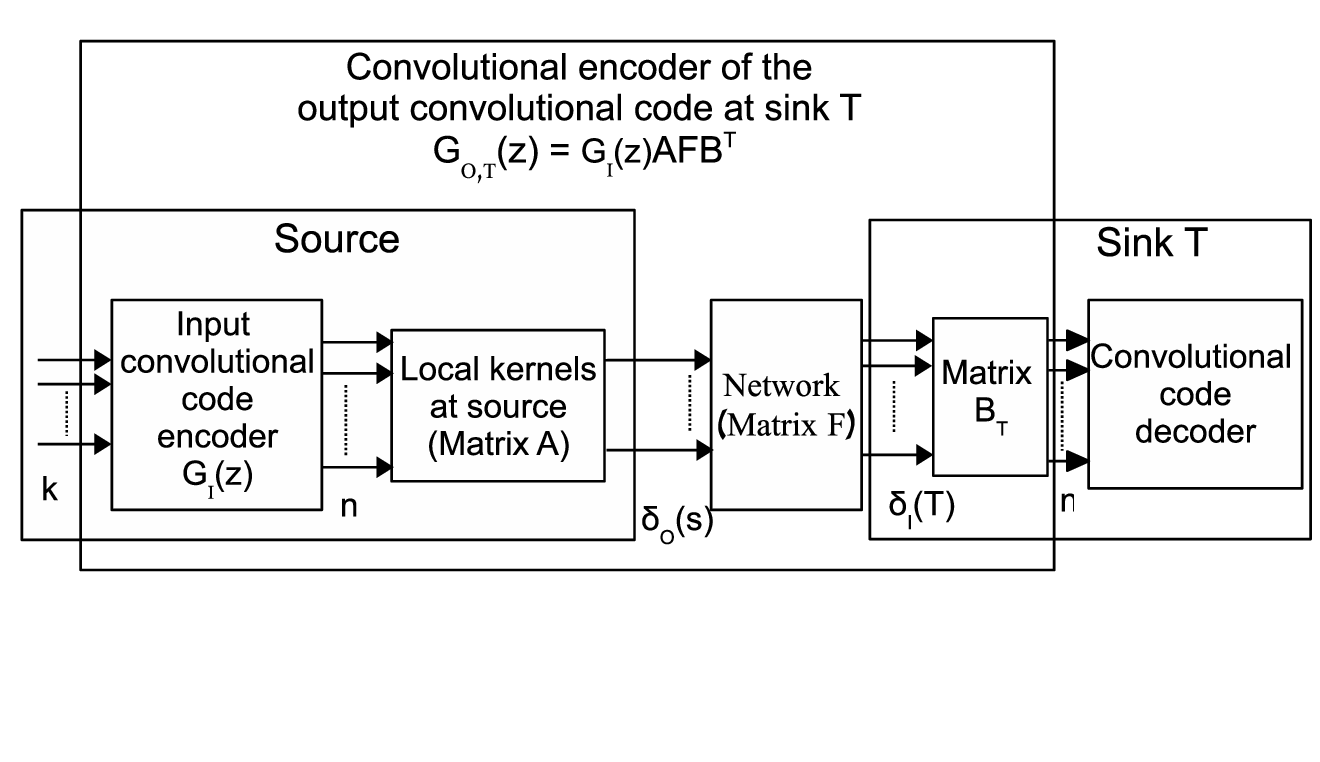
Thus, as can be seen from the Example 1, the source node implements a convolutional code, and maps the encoded symbols into its outgoing symbols. The network maps these symbols from the source to symbols at the receivers. Each of the receivers hence sees a different convolutional code which might have different distance properties and different degrees ($\delta$). Fig. 2 illustrates the entire system for a particular sink.

An error pattern $\rho,$ as stated previously, is a subset of ${\cal E}$ which indicates the edges of the network in error. An error vector $\boldsymbol{w}$ is a $1\times|{\cal E}|$ vector which indicates the error occurred at each edge. An error vector is said to match an error pattern $(\text{i.e }\boldsymbol{w}\in\rho)$ if all non-zero components of $\boldsymbol{w}$ occur only on the edges in $\rho$. An error pattern set $\Phi$ is a collection of subsets of ${\cal E}$, each of which is an error pattern. Therefore we have the formulation as follows.

Let $\boldsymbol{x}\in\mathbb{F}_{q}^{n}$ be the input to the network at any particular time instant, and let $\boldsymbol{w}\in F_{q}^{|{\cal E}|}$ be the error vector corresponding to the network-errors that occurred in the same particular instant. Then, the output vector, $\boldsymbol{y}\in\mathbb{F}_{q}^{n}$, at that instant at any particular sink $T\in\cal T$ can be expressed as

In this section, we briefly discuss and give some results regarding the bounded distance decoding of convolutional codes, reinterpreting results from [18] for our context.

For the convolutional encoder with $c$ encoded output symbols and $b$ input (information) symbols, starting at some state in the trellis, we shall denote every such $c$ output symbol durations as a segment of the trellis of the convolutional code. Each segment can be identified by an integer, which is zero at the start of transmission and incremented by $1$ for every $c$ output symbols henceforth.

Let $\cal C$ be a rate $b/c$ convolutional code with a generator matrix $G(z).$ Then corresponding to the information sequences $\boldsymbol{u}_{0},\boldsymbol{u}_{1},..(\boldsymbol{u}_{i}\in\mathbb{F}_{q}^{b})$ and the code sequence $\boldsymbol{v}_{0},\boldsymbol{v}_{1},...(\boldsymbol{v}_{i}\in\mathbb{F}_{q}^{c})$, we can associate an encoder state sequence $\boldsymbol{\sigma}_{0},\boldsymbol{\sigma}_{1},..$, where $\boldsymbol{\sigma}_{t}$ indicates the content of the delay elements in the encoder at a time $t.$We define the set of $j$ output symbols as $\boldsymbol{v}_{[0,j)}:=\left[\boldsymbol{v}_{0},\boldsymbol{v}_{1},...,\boldsymbol{v}_{j-1}\right].$ We define the set $S_{d_{free}}$ consisting of all possible truncated code sequences $\boldsymbol{v}_{[0,j)}$ $\forall$ $j$ of weight less than $d_{free}({\cal C})$ that start in the zero state as follows:

where $w_{H}$ indicates the Hamming weight over $\mathbb{F}_{q}.$ Clearly the definition of $S_{d_{free}}$ excludes the possibility of a zero state in between (in the event of which $w_{H}\left(\boldsymbol{v}_{[0,j)}\right)\geq d_{free}({\cal C})$), i.e, $\boldsymbol{\sigma}_{t}\neq\boldsymbol{0}\text{ for any t such that }0<t\leq j.$ We have that the set $S_{d_{free}}$ is invariant among the set of minimal convolutional encoders. We now define

which thereby can be considered as a code property because of the fact that $S_{d_{free}}$ is invariant among minimal encoders. Then, we have the following proposition:

For the given network with a single source that has to multicast information to a set of sinks, $n$ being min-cut of the multicast connections, a $n$-dimensional network code in place over a sufficiently large field $F_{q}$ (for which we provide a bound in Subsection IV-E) of characteristic $p$, we provide a construction for a convolutional code for correcting errors with patterns in a given error pattern set. This is the main contribution of this work. The construction is as follows.

1. 1.

   Let $M_{T}=AF_{T}$ be the $n\times n$ network transfer matrix from the source to any particular sink $T\in{\cal T}$. Let $\Phi$ be the error pattern set given. Then we compute the following sets.

2. 2.

   Let the set of all error vectors having their error pattern in $\Phi$ be

   $${\cal W}_{\Phi}=\bigcup_{\rho\in\Phi}\left\{\boldsymbol{w}=(w_{1},w_{2},...,w_{|{\cal E}|})\in\mathbb{F}_{q}^{|{\cal E}|}\text{ }|\text{ }\boldsymbol{w}\in\rho\right\}.$$

3. 3.

   Let

   $${\cal W}_{T}:=\left\{\boldsymbol{w}F_{T}\text{ }|\text{ }\boldsymbol{w}\in{\cal W}_{\Phi}\right\}$$

   be computed for each sink $T$. This is nothing but the set of n-length resultant vectors at the sink $T$ due to errors in the given error patterns $\rho\in\Phi$.

4. 4.

   Let

   $${\cal W}_{s}:=\bigcup_{T\in{\cal T}}\left\{\boldsymbol{w}_{{}_{T}}M_{T}^{-1}\text{ }|\text{ }\boldsymbol{w}_{{}_{T}}\in{\cal W}_{T}\right\}$$

   be computed. This is the set of all $n$ length input vectors to the network that would result in the set of output vectors given by ${\cal W}_{T}$ at sink $T$, for each sink $T$.

5. 5.

   Given a vector $\boldsymbol{y}\in\mathbb{F}_{q}^{m}$ (for some positive integer $m$), let $w_{H}(\boldsymbol{y})$ denote the Hamming weight of $\boldsymbol{y}$, i.e., the number of non-zero elements of $\boldsymbol{y}$. Let

   $$t_{s}=\max_{\boldsymbol{w}_{s}\in{\cal W}_{s}}w_{H}(\boldsymbol{w}_{s}).$$

   (2)

6. 6.

   Choose an input convolutional code ${\cal C}_{s}$ with free distance at least $2t_{s}+1$.

Let $G_{I}(z)$ be the $k\times n$ generator matrix of the input convolutional code, ${\cal C}_{s}$, obtained from the given construction. Let $G_{O,{T}}(z)=G_{I}(z)M_{T}$ be the generator matrix of the output convolutional code, ${\cal C}_{T}$, at sink $T\in{\cal T}$, with $M_{T}$ being its network transfer matrix. Each sink can choose between two decoding methods based on the free distance ($d_{free}({\cal C}_{T})$) and $T_{d_{free}}({\cal C}_{T})$ of its output convolutional code as follows:

Case-A: This case is applicable in the event of both of the following two conditions are satisfied.

and

In this case, the sink $T$ performs minimum distance decoding directly on the trellis of the output convolutional code, ${\cal C}_{T}$.

Case-B: This case is applicable if either of the following two conditions are satisfied.

or

This method involves additional processing at the sink, i.e, matrix multiplication. We have the following formulation at the sink $T$. Let

represent the output sequences at sink $T$, where

$\boldsymbol{u}(z)$ being the $k$ length vector of input sequences, and

represent the corresponding error sequences. Now, the output sequences are multiplied with the inverse of the network transfer matrix $M_{T}$, so that decoding can be done on the trellis of the input convolutional code. Hence, we have

where $\boldsymbol{w^{\prime}}(z)=\left[w_{1}^{\prime}(z)\text{ }\text{ }w_{2}^{\prime}(z)\text{ }\text{ }...\text{ }\text{ }w_{n}^{\prime}(z)\right]$ now indicate the set of modified error sequences that are to be corrected. Then the sink $T$ decodes to the minimum distance path on the trellis of the input convolutional code.

In this subsection we prove a main result of the paper given by Theorem 3 which characterizes the error correcting capability of the code obtained via the construction of Subsection IV-B. Before proving the following theorem, we recall the following observation that in every network use, $n$ encoded symbols which is equal to the number of symbols corresponding to one segment of the trellis, are to be multicast to the sinks.

References

- [1] R. Ahlswede, N. Cai, R. Li and R. Yeung, “Network Information Flow”, IEEE Transactions on Information Theory, vol.46, no.4, July 2000, pp. 1204-1216.
- [2] N. Cai, R. Li and R. Yeung, “Linear Network Coding”, IEEE Transactions on Information Theory, vol. 49, no. 2, Feb. 2003, pp. 371-381.
- [3] R. Koetter and M. Medard, “An Algebraic Approach to Network Coding”, IEEE/ACM Transactions on Networking, vol. 11, no. 5, Oct. 2003, pp. 782-795.
- [4] Ho, T. Medard, M. Koetter, R. Karger, D.R. Effros, M. Jun Shi and Leong, B., “A Random Linear Network Coding Approach to Multicast”, IEEE Transactions on Information Theory, vol. 52, no. 10, Oct. 2006, pp. 4413-4430.
- [5] Raymond W. Yeung and Ning Cai, “Network error correction, part 1 and part 2”, Comm. in Inform. and Systems, vol. 6, 2006, pp. 19-36.
- [6] Zhen Zhang, “Linear network-error Correction Codes in Packet Networks”, IEEE Transactions on Information Theory, vol. 54, no. 1, Jan. 2008, pp. 209-218.
- [7] Shenghao Yang and Yeung, R.W., “Refined Coding Bounds for network error Correction”, IEEE Information Theory Workshop on Information Theory for Wireless Networks, July, 2007, pp. 1-5.
- [8] R. Koetter and F.R. Kschischang, “Coding for Errors and Erasures in Random Network Coding”, IEEE Transactions on Information Theory, vol. 54, no. 8, Aug. 2008, pp.3579-3591.
- [9] D. Silva,F. R Kschischang, and R. Koetter, “A Rank-Metric Approach to Error Control in Random Network Coding”, IEEE Transactions on Information Theory, vol. 54, no. 9, Sept. 2008, pp. 3951-3967.
- [10] E. Erez and M. Feder, “Convolutional network codes”, IEEE International Symposium on Information theory, Chicago, Illinois, USA, June 2004, pp. 146.
- [11] N. Cai, R. Li, R. Yeung, Z. Zhang, “Network Coding Theory”, Foundations and Trends in Communications and Information Theory, vol. 2, no.4-5, 2006.
- [12] S. R. Li and R. Yeung, “On Convolutional Network Coding”, IEEE International Symposium on Information Theory, Seattle, Washington, USA, July 2006, pp. 1743-1747.
- [13] C. Fragouli, and E. Soljanin, “A connection between network coding and convolutional codes”, IEEE International Conference on Communications, Paris, France, 2004, vol. 2, pp. 661-666.
- [14] R. Johannesson and K.S Zigangirov, Fundamentals of Convolutional Coding, John Wiley, 1999.
- [15] G. D. Forney, “Bases of Rational Vector Spaces with applications to multivariable linear systems”, SIAM J. Contr., vol. 13, no. 3, 1975, pp. 493-520.
- [16] J. Rosenthal and R. Smaradanche, “Maximum Distance Separable Convolutional Codes”, Appl.Algebra Engrg. Comm. Comput., vol. 10, no. 1, June 1999, pp. 15-32.
- [17] J. Rosenthal, H. Gluesing-Luerssen, and R.Smaradanche, “Construction of MDS convolutional codes”, Appl.Algebra Engrg. Comm. Comput., vol. 47, no. 5, July 2001, pp. 2045-2049.
- [18] J.M.Jensen and I. S. Reed, “Bounded distance coset decoding of convolutional codes”, IEE Proceedings, vol. 133, no. 5, pp. 1046-1060, 1986.