ENERGY LOSS IN A STRONGLY COUPLED THERMAL MEDIUM AND THE GAUGE-STRING DUALITY
Abstract
We review methods developed in the gauge-string duality to treat energy loss by energetic probes of a strongly coupled thermal medium. After introducing the black hole description of the thermal medium, we discuss the trailing string behind a heavy quark and the drag force that it implies. We then explain how to solve the linearized Einstein equations in the presence of the trailing string and extract from the solutions the energy density and the Poynting vector of the dual gauge theory. We summarize some efforts to compare these calculations to heavy ion phenomenology.
This manuscript was typeset using a class file inherited from ws-ijmpe.cls. Ws-imjpe.cls is copyrighted to World Scientific Publishing Company.
1 Introduction
A long-standing hope, as yet unrealized, is that quantum chromodynamics (QCD) will be reformulated as a string theory. The gauge-string duality[1, 2, 3] provides the closest approach to that goal so far attained. It provides useful computational methods for studying strongly coupled gauge theories. The theory that is most accessible via these methods is super-Yang-Mills theory (SYM) in the limit of a large number of colors and large ’t Hooft coupling.11 1 super-Yang-Mills theory is a gauge theory whose matter content consists of gluons, four Majorana fermions in the adjoint representation of the gauge group, and six real scalars, also in the adjoint representation. All the fields are related to one another by the supersymmetry, which completely fixes the Lagrangian once the gauge group and gauge coupling are chosen. Our interest is in the gauge group . Aspects of the progress in using the gauge-string duality to understand QCD have recently been reviewed at a pedestrian level.[4] The aim of the current article is a more focused review of efforts to understand energy loss by energetic probes of a thermal medium in a strongly coupled gauge theory, such as SYM, which has a string theory dual; and to review how energy loss in SYM can be compared to energy loss in QCD.
At least in simple cases like SYM, the response of an infinite, static, strongly coupled thermal medium to an energetic probe can be presumed to be hydrodynamical far from the probe, because hydrodynamic perturbations are the only long-wavelength modes available. In an infinite, interacting thermal medium, there is no radiation, because there are no asymptotic states. In a strongly coupled medium, it is not clear that there is a gauge-invariant distinction between collisional energy loss and radiative energy loss. So the main questions are:
- 1.
What is the rate of energy loss from an energetic probe?
- 2.
What is the hydrodynamical response far from the energetic probe?
- 3.
What gauge-invariant information can be extracted using the gauge-string duality about the non-hydrodynamic region near the probe?
- 4.
Do the rate and pattern of energy loss have some meaningful connection to heavy ion phenomenology?
In section 2 we briefly review the dual description of the thermal state of SYM as an AdS5-Schwarzschild black hole. The reader interested in a more extensive discussion of the AdS/CFT duality is referred to various reviews in the literature.[5, 6, 7] In section 3 we explain how to describe heavy quarks in SYM using strings in AdS5, and in section 4 we extract the drag force acting on the quark via an “obvious” and “alternative” identification of parameters between SYM and QCD. Also in section 4, we consider how the string theory estimates of drag force relate to the measured nuclear modification factor for heavy quarks.
The response of the stress-tensor to the motion of the quark is dual to the metric perturbations around an AdS black hole. These are studied in section 5, where we also discuss how the metric perturbations map into the stress tensor of the plasma. In section 6 we provide analytic approximations to the stress tensor both near to the moving quark and far from it. The full numerical solution is described in section 7, and its application to heavy-ion phenomenology can be found in section 8. In A we provide a glossary of mathematical notations used in the main text.
2 The thermal medium as a black hole
super-Yang-Mills theory at finite temperature can be described in terms of D3-branes near extremality.[8] D3-branes are dimensional objects on which strings may end.[9, 10] Each string can end on one of the D3-branes, which eventually gives rise to the gauge symmetry of SYM.[11] Having a non-vanishing tension, D-branes themselves warp the spacetime around them. The near horizon geometry produced by the D3-branes is AdS5-Schwarzschild times a five-sphere, threaded by units of flux of the self-dual Ramond-Ramond five-form of type IIB supergravity.[12] For most calculations of interest to us in this review, one can ignore the five-sphere and work just with the five non-compact dimensions.
Our starting point is the Einstein equations of type IIB supergravity in the non-compact directions, which can be recovered from the action
| (1) |
Here is the five-dimensional gravitational coupling, , and is the radius of the . Standard relations based ultimately on the quantized charge of the D3-brane lead to
| (2) |
AdS5-Schwarzschild is a solution of the Einstein equations following from (1). Its line element is
| (3) |
where the “blackening function” is given by
| (4) |
In this coordinate system, the conformal boundary of AdS5 is located at .
The AdS5-Schwarzschild solution has a horizon at , whose temperature is
| (5) |
According to the gauge-string duality, the temperature of the horizon (5) is also the temperature of the thermal medium in the dual gauge theory.[3] This medium is infinite and static. Its energy density equals the mass per unit coordinate volume, , of the black hole, and its pressure can also be straightforwardly computed as minus the free energy of the black hole. To leading order in the number of colors and the ’t Hooft coupling , one finds
| (6) |
These relations reflect the conformal invariance of super-Yang-Mills theory, which is exact even at finite and . If we send , or equivalently , we end up with a pure AdS5 geometry and no black hole.
Perturbations of the AdS5-Schwarzschild black hole with wavelengths much longer than are described by relativistic fluid dynamics,[13, 14] and the viscosity is known to be remarkably small:[15]
| (7) |
again to leading order in the limit of large and .
In summary: A thermal medium of super-Yang-Mills theory can be represented as a black hole in AdS5 in the limit of large and large ’t Hooft coupling. Relations between the radius of AdS5 and the five-dimensional gravitational coupling, between the temperature and the position of the horizon, between the energy density and the temperature, and between the viscosity and the entropy density, can all be derived starting from ten-dimensional type IIB string theory.
3 The trailing string
super-Yang-Mills theory has no fundamentally charged quarks. Instead, its field content is the gluon and its superpartners under supersymmetry: namely, four Majorana fermions and six real scalars, all in the adjoint representation of . The AdS5 description of SYM makes no direct reference to these colored dynamical fields. The magic of AdS/CFT is to replace the strong coupling dynamics of open strings, whose low-energy quanta participate in the gauge theory, with the gravitational dynamics of closed strings (gravitons, for example) in a weakly curved background. For example, as we saw in section 2, a finite temperature bath in the gauge theory is replaced by a black hole in AdS5. The absence of colored degrees of freedom in the gravitational theory makes it less than obvious how to discuss energetic colored probes of the medium.
A clue comes from the treatment of Wilson loops in the gauge-string duality.[16, 1] A static, infinitely massive, fundamentally charged quark can be represented as a string hanging straight down from the boundary of AdS5, at , into the horizon. There is no contradiction with the previous statement that super-Yang-Mills has no fundamentally charged quarks, because the quark is an external probe of the theory, not part of the theory. An anti-fundamentally charged quark is represented in the same way as a quark, except that the string runs the other way. (In type IIB string theory, strings are oriented, so this statement makes sense.) If a quark and an anti-quark are both present, it is possible for the strings running down into AdS5 to lower their total energy by connecting into a shape like a catenary. From the point of view of the boundary theory, the string configuration gives rise to an attractive potential with a dependence, as conformal invariance says it must.
Let’s go back to a single isolated quark—which makes sense in even at zero temperature because there is no confinement. The string dual to the quark can be described by its embedding in AdS5. The two-dimensional spacetime manifold swept out by the string is called a worldsheet and can be parameterized by two coordinates. If we use and to parameterize the string worldsheet, then the string in AdS5, or in AdS5-Schwarzschild, dual to a static quark at , is described by the equation
| (8) |
This is a solution to the string equations of motion with boundary conditions such that the string endpoint on the boundary is stationary. By symmetry, (8) is the only possible solution with these boundary conditions. In the absence of a medium, it must be that the description of a moving quark can be obtained by performing a Lorentz boost on the description of a static quark. If the boost is in the direction, and we continue to use and to parameterize the worldsheet, then the equations describing the string dual to a quark moving in the absence of a medium are
| (9) |
where is the velocity of the quark and .22 2 It would be more proper to use in place of , and reserve the notation for . However, it simplifies notation to set for , and we will do this consistently. Given that (8) solves the equations of motion of classical string theory, it’s guaranteed that (9) does too, because the equations are invariant under the boost in the direction, and the line element (3) with is invariant under any boost acting on the coordinates.
When , signaling the presence of a medium, a moving quark is not the same as a static one. Naively, one might nevertheless try to represent the moving quark in terms of the string shape described in (9). Let’s see why this is problematic. String dynamics is defined in terms of the metric on the worldsheet. We chose to parameterize the worldsheet by and , but any coordinates could have been chosen. For a general embedding of a string worldsheet into spacetime, the worldsheet metric is
| (10) |
What (10) says is that times and distances along the string are measured the same way as in the ambient spacetime. Using and the ansatz (9), one immediately finds
| (11) |
This shows that the direction on the worldsheet is always spacelike and that the direction is timelike only when . Using (4), this condition is equivalent to
| (12) |
The part of the string worldsheet with is purely spacelike, which means that the string is locally moving faster than the speed of light. This does not make sense if we are aiming to describe the classical dynamics of a string moving in real Minkowski time.
There is a simpler way to arrive at (12): any trajectory of a point particle in the bulk of AdS5-Schwarzschild with must be spacelike—that is, the speed of the particle will exceed the local speed of light—if the inequality is violated. This conclusion holds even when there are other components of the velocity, but the inequality is sharp only in the case where there aren’t.
Physically, what we learn from (12) is that it is harder and harder to move forward as one approaches the horizon. This evokes the idea that there must be some drag force from the medium. But how does one get at that drag force? An answer was provided by two groups,[17, 18] and closely related work on fluctuations appeared at the same time.[19] The string does not hang straight down from the quark: rather, it trails out behind it. If the shape is assumed not to change as the quark moves forward, and if it respects the symmetry rotating the coordinates, then it must be specified by a small variant of (9):
| (13) |
for some function . If we insist that the quark’s location on the boundary is , then we must have as .
To determine , one must resort to the classical equations of motion for the string. These follow from the action
| (14) |
where . The parameter is related to and the ’t Hooft coupling by
| (15) |
Here we define , so that a quantity analogous to the coupling in QCD is . The classical equations of motion following from the action (13) take the form
| (16) |
where
| (17) |
is the momentum current on the worldsheet conjugate to the position . Plugging (13) into (17), one straightforwardly finds that
| (18) |
where is a constant of integration. In order for to be real, the right hand side of (18) must be real. There are three ways this can happen in a manner consistent with the assumption of steady-state behavior:33 3 Technically, there is a fourth way, but its significance is obscure to us. A string can lead down to in the shape of the trailing string, (20), and then turn around and retrace its path back up again. The energy localized at the kink must grow linearly with time, which means that this configuration is not quite a steady-state solution.
- •
One can choose . This leads to , which shows that (9) is formally a solution of the equations of motion. But it is not a physical solution—at least, not in the context of classical motions of a string—because of the problem with the signature of the worldsheet metric. The action for this solution is complex.
- •
One can arrange for the worldsheet never to go below , and choose small enough that the denominator inside the square root in (18) is always positive. There is indeed a one-parameter family of such solutions, and they describe a heavy quark and anti-quark in a color singlet state propagating without drag (at the level of the current treatment), one behind the other. Similar states were studied by other groups,[20, 21, 22] but they do not capture the dynamics of a single quark propagating through the plasma, so we do not consider them further here.
- •
One can choose
(19) so that the denominator inside the square root in (18) changes sign at the same value of as the numerator, namely , rendering the ratio inside the square root everywhere positive and finite. Choosing the sign that makes positive means that the string trails out in front of the quark instead of behind it. Although this is technically a solution, it does not describe energy loss and should be discarded. Choosing negative leads to the trailing string solution that we are interested in. Eq. (18) then straightforwardly leads to
(20) where we have introduced a rescaled depth variable,
(21)
There is another way to justify the choice of the minus sign, not the plus sign, in (19):[23] The solution (20) is non-singular at the future event horizon, whereas the solution one would get with the opposite sign choice is singular. To understand this point, it is convenient to pass to Kruskal coordinates, defined implicitly by the equations
| (22) |
In the region outside the horizon, and , while in the region inside the future horizon, and . The trailing string solution (13), with given by (20), can be extended to a non-singular solution over the union of these two regions:
| (23) |
Thus, the logarithmic singularity in at (meaning ) is a singularity not at the future horizon, which is at , but at the past horizon, which is at . Reversing the sign choice in (19) would lead to a solution that is singular at the future horizon but not the past horizon. Causal dynamics in the presence of a black hole horizon can generally be described in terms of functions which are smooth at the future horizon.
At the level of our presentation, it has been assumed rather than demonstrated that the trailing string is a stable, steady-state configuration representing the late time behavior of a string attached to a moving quark on the boundary of AdS5- Schwarzschild. In fact, this has been fairly well checked.[17, 24]
The description we have given of the trailing string is not limited to Schwarzschild black holes in AdS5. One may extend this analysis to various other black hole geometries which asymptote to AdS5 near their boundary.[25, 26, 27, 28, 29, 30] These geometries describe theories which are deformations of SYM. The literature also includes a discussion of the distribution of energy along the string[31] and an interpretation of the shape of the string in terms of a rapid cascade of strongly coupled partons.[32]
4 The magnitude of the drag force
As we explained in the previous section, an infinitely massive, fundamentally charged quark moving at speed in the direction through an infinite, static, thermal medium of super-Yang-Mills theory can be described at strong coupling in terms of the trailing string solution (20). The quark cannot slow down because it has infinite mass. However, it does lose energy and momentum at a finite, calculable rate. In five-dimensional terms, this energy can be thought of as flowing down the string toward the black hole horizon. In four-dimensional terms, energy and momentum emanates from the quark and eventually thermalizes. To calculate the four-momentum delivered from the quark to the bath over a time , one can integrate the conserved worldsheet current of spacetime energy-momentum over an appropriate line-segment on the worldsheet. should cover a time interval , and it can be chosen to lie at a definite depth in AdS5. The four-momentum is44 4 There is an explicit minus sign in (24) which doesn’t appear in the analogous equation of one of the original works.[18] This is due to use of the variable, which increases as one goes deeper into AdS5, instead of the variable, which increases as one goes out toward the boundary.
| (24) |
Because the trailing string is a steady-state configuration, four-momentum is lost at a constant rate:
| (25) |
In particular, the drag force can be defined as
| (26) |
Using (5) and (15), one obtains
| (27) |
If, instead of an infinitely massive quark, we consider a quark with finite but large mass , then using the standard relativistic expression
| (28) |
leads to
| (29) |
It has been explained[17] that (28) receives corrections when a finite mass quark is described as a string ending at a definite depth on a D7-brane. While these corrections are interesting, it would take us too far from the main purpose of this review to give a proper explanation of how the D7-branes modify the physics. Our discussion is formal because we derived the result (27) in the strict limit and then applied it to finite mass quarks.
From (29) it is clear that the drag force causes the momentum of a quark to fall off exponentially:
| (30) |
In order to make a physical prediction for QCD, we must plug in sensible values for , , and . The effective quark mass in the thermal medium is already non-trivial to specify precisely, but for charm and for bottom are reasonably representative values which were used in a recent phenomenological study.[33] We will review here two approaches[34] to specifying and . The first approach, used earlier in a calculation of the jet-quenching parameter from a lightlike Wilson loop in super-Yang-Mills theory,[35] is to identify the temperature with the temperature , and then identifying the gauge coupling of super-Yang-Mills with the gauge coupling of QCD evaluated at temperatures typical of RHIC. Because of the proximity of the confinement transition, has substantial uncertainty. A standard choice is , corresponding to . With the number of colors set equal to , one finds . We will refer to this as the “obvious scheme.”
The second approach, called the “alternative scheme,” is based on two ideas. The first idea is that it may make more sense to compare SYM to QCD at fixed energy density than fixed temperature. SYM has , and so does QCD, approximately: this approximation is surprisingly good for , according to lattice data.[36] But the constant of proportionality is about times bigger for SYM than for QCD.55 5 This mismatch has previously been stated[34] as a factor of rather than . Some uncertainty exists on both the SYM and the QCD sides, because of finite coupling effects and time discretization, respectively; but is probably closer to the true figure. That is, SYM has about times as many degrees of freedom as QCD above the confinement transition. So implies . This identification leads to a suppression of by a factor of relative to the obvious scheme. The second idea behind the alternative scheme is that the ’t Hooft parameter in string theory can be determined by comparing the static force between a quark and an anti-quark, as calculated in string theory, to the same force calculated in lattice gauge theory. The string theory calculation is based on a U-shaped string connecting the quark and the anti-quark. This string pulls on the static quarks in a fashion that is similar to how the trailing string pulls on a moving quark. The lattice calculation is based on computing the excess free energy due to the presence of an external quark and anti-quark in a thermal bath. There is a significant difficulty: in the simplest string theory calculation, based only on the U-shaped string, the force between the quark and anti-quark vanishes for separations larger than some limiting distance , and this distance is quite small: when (corresponding to ). It has been pointed out[37] that exchange of closed strings between two long strings describing the quark and anti-quark at separations contribute to the quark-anti-quark force at the same order in as the U-shaped string. Unfortunately, it is hard to compute the contribution of closed string exchange. The approach[34] is therefore to match the U-shaped string computation to lattice data[38] near the limiting distance . The result of this matching is .
| \topruleScheme | |||||||||
| MeV | MeV | GeV | GeV | fm | fm | ||||
| \colruleobvious | 250 | 15 | 1.5 | 4.8 | 0.69 | 2.2 | |||
| alternative | 195 | 5.6 | 5.5 | 1.5 | 4.8 | 2.1 | 6.8 | ||
| \botrule |
\tabmarka We set because this is a typical temperature scale for heavy ion collisions at .
\tabmarkb We use for QCD.
As we show in table 1, heavy quark relaxation times and are remarkably short when one uses the obvious scheme, and somewhat larger in the alternative scheme. The uncertainties in and are substantial: even if one accepts the ideas behind the alternative scheme, one should probably regard the resulting relaxation times as uncertain by a factor of .
An experimental study[39] favors a model[40] in which is roughly at , as estimated from plots from a detailed exposition of that model.[41] This seems to indicate that the string theory estimates of and , even in the alternative scheme, are too short. However, the results of a recent phenomenological study[33] favor a range of parameters that is consistent with the string theory predictions translated to QCD using the alternative scheme.
Let us briefly review the recent study.[33] The starting point is the Langevin equation, which in the Itô discretization scheme takes the form
| (31) |
Here is a stochastic force, assumed to be Gaussian and uncorrelated from one time-step to the next. The strength of the stochastic force is related to the drag coefficient by demanding that the relativistic Maxwell-Boltzmann distribution is preserved by the time evolution (31). Ordinary relativistic kinematics, , are assumed. It is also assumed that
| (32) |
where is a dimensionless quantity with no dependence. Evidently, . The temperature in (32) is , whereas the temperature in (30) is . Comparing these two equations, one finds that the string theory prediction is
| (33) |
The alternative scheme value in (33) is fractionally larger than the one quoted in the study under discussion,[33] due to the use here of the factor for the ratio of degrees of freedom between SYM and QCD, as compared to in previous work.[34] (It is a numerical coincidence that the dimensionless factor is the same, in the alternative scheme, as in femtometers when .)
The next step of the study[33] is to compare Langevin dynamics of heavy quarks in a hydrodynamically expanding plasma to PHENIX[39] and STAR[42] data on the nuclear modification factor for non-photonic electrons—meaning electrons and positrons coming from decays of heavy-quark mesons. Because of the treatment of hadronization, the theoretical results are deemed trustworthy only when the transverse momentum of the non-photonic electron is at least .66 6 The electron carries only a fraction of the of the charm quark that led to its production. This fraction varies, but a reasonable rule-of-thumb value is . For fairly central collisions (impact parameter ), agreement between theory (using the alternative scheme) and experiment is best for between and : see figure 1.
Thus the prediction (33) of string theory in the alternative scheme can reasonably be said to agree with data to within the uncertainties of the calculations. These uncertainties stem in large part from the difficulty of comparing SYM to QCD; however, it is also clear that the treatment of hadronization is a significant hurdle.[33]
Fluctuations of the trailing string[19, 24, 23, 43] provide direct access to the stochastic forces in (31). In the non-relativistic limit, the size of these forces, relative to the drag force, is exactly what is needed to equilibrate to a thermal distribution. Indeed, the original calculations of drag force[17, 18] and stochastic forces[19] were done independently. For relativistic quarks, the stochastic forces are enhanced by powers of , including enhancement of longitudinal stochastic forces by the startlingly large factor . This is larger by than what is needed to equilibrate to a thermal distribution. Another issue is that the correlation time for these stochastic forces grows with velocity: based on results for the relevant Green’s function[24] one may estimate
| (34) |
If we use as a criterion of validity for the Langevin dynamics, then we get a limit on the Lorentz boost factor:
| (35) |
Approximately the same inequality arises from demanding that when the string ends on a D7-brane, its endpoint should not move superluminally. The same inequality, but with replaced by some fixed scale , also arises from demanding that the worldsheet horizon[24, 23] should be at a depth in AdS5 corresponding to a scale where the dynamics of QCD is far from weakly coupled. Plugging in numbers in the alternative scheme, with and , one finds that . This inequality should be understood as quite a rough estimate, because of the quadratic dependence on the quantity which is only qualitatively defined. For a charm quark, the corresponding limit on the transverse momentum of the non-photonic electron is . This is well in excess of the highest momentum for which there are statistically significant data; moreover, for more than a few , bottom quarks dominate, and for them the bound translates to for non-photonic electrons. The upshot is that heavy quarks at RHIC do not obviously fall outside the regime of validity of a self-consistent Langevin treatment based on the trailing string—except for the troublesome scaling of longitudinal stochastic forces as , whose consequences, we feel, are ill-understood.
In another study,[44] it is argued that energy loss in the perturbative and strongly coupled regimes have experimentally distinguishable signatures for large enough transverse momenta, , which will be attained at the LHC. A convenient observable that distinguishes between predictions of string theory and perturbative QCD is the ratio of the nuclear modification factors for and quarks,
| (36) |
In particular, the drag force formula (29) implies that at large enough , one has
| (37) |
where we used the bottom and charm masses quoted right after equation (30). In contrast, perturbative QCD predicts that
| (38) |
at large , where is a relevant momentum scale. So according to perturbative QCD, should approach unity at large . At sufficiently large , the trailing string treatment presumably fails, and perturbative QCD presumably is correct. But as discussed following (35), it is difficult to give a good estimate of the characteristic value of where the trailing string fails. Absent a reliable estimate of the characteristic , the upshot is that if the measured is significantly below the perturbative prediction, the trailing string should be considered as a candidate explanation.
5 The perturbed Einstein equations
Given that an external quark dual to the trailing string described in section 3 experiences drag, one might ask what happens to the energy that the quark deposits in the medium. At scales much larger than the inverse temperature, one expects the excitations present in the medium due to interactions with the moving quark to be well-described by linearized hydrodynamics. Earlier investigations of linearized hydrodynamics revealed the presence, for generic sources, of both a sonic boom and a diffusion wake.[45] The sonic boom is a directional structure, which, in an ideal fluid, is concentrated on the Mach cone, but in a real fluid there is broadening because of viscous effects. It appears only when the probe is moving faster than the speed of sound in the medium, and it comes from constructive interference among spherical waves sourced by the quark along its trajectory. The diffusion wake is a flow of the medium behind the quark in the direction of the quark’s motion. It too is broadened by viscous effects. We will discuss the hydrodynamic limit in more detail in section 6.1.2.
Apart from a qualitative understanding of energy loss at large distances, little is known a priori about what happens, for example, at small distances close to the quark. An all-scales description can be achieved using the gauge-string duality, where one computes the disturbances in the stress-energy tensor due to the presence of the quark. This was done in a series of papers.[46, 47, 48, 49, 50, 51, 52, 53] The linearized response of the lagrangian density in the dual field theory was also computed in Fourier space.[54, 55] The purpose of this section and the next two is to present a reasonably self-contained summary of how the gauge theory stress-energy tensor is computed starting from the trailing string. A visual summary of the main elements of the computation is shown in figure 2.
In the context of the AdS/CFT duality, the stress-energy tensor of the boundary theory is dual to fluctuations of the metric in the bulk. So in order to compute the expectation value of , one first needs to compute to linear order the backreaction of the string describing the quark on the metric. Non-linear corrections to the Einstein equations will be suppressed by . The total action describing both the string and the metric is , which one can write as
| (39) |
where is the embedding function of the string in AdS5-Schwarzschild. In a gauge where we parameterize the string worldsheet by , is given by
| (40) |
with as given in (20). The equations of motion following from (39) are just Einstein’s equations:
| (41) |
where
| (42) |
is the bulk stress-energy tensor of the trailing string.
To compute the backreaction of the string on the metric, we write
| (43) |
where is the unperturbed AdS5-Schwarzschild metric given in (3), and plug this into (41) to obtain the linearized equations of motion for the metric perturbations . The resulting equations take the form
| (44) |
where and is the differential operator given by[56]
| (45) |
The covariant derivatives, the Riemann and Ricci tensors, and the Ricci scalar appearing in (45) are computed using the background metric , and we have denoted .
For a steady-state solution of (44), depends on and only through the combination . We therefore pass to co-moving Fourier space variables by writing
| (46) |
where we have defined the dimensionless wavevector . We make a similar expansion for . In Fourier space, (44) can then be written as
| (47) |
with being given by
| (48) |
where is the rescaled depth coordinate defined in (21), but the tensor components are given in the coordinate system. The explicit form of is too complicated to be reproduced here.
We will decouple equations (47) by passing to a gauge where , which we will refer to as “axial gauge.” Note that leaves some residual gauge freedom. We will discuss this shortly.
The rest of this section is organized as follows. In section 5.1 we explain how to decouple equations (47). In section 5.2 we explain the boundary conditions needed to solve these equations. Lastly, in section 5.3 we explain how the one-point function of the SYM stress-energy tensor is related to the asymptotic behavior of the metric perturbations near .
5.1 Metric perturbations in axial gauge
As mentioned above, we choose a gauge where , and let
| (49) |
Rotational symmetry around the direction of motion of the quark allows us to set with . Defining
| (50) |
one can form the following linear combinations of metric perturbations:
| (51a) | ||||
| (51b) | ||||
| (51c) | ||||
| (51d) | ||||
| (51e) | ||||
| (51f) | ||||
| (51g) | ||||
Using these new variables, the Einstein equations (47) decouple into five sets:[46]
| (52a) | |||
| (52b) | |||
| (52c) | |||
| (52d) | |||
| (52e) | |||
| (52f) | |||
| (52g) | |||
| (52h) |
In (52), , , , , and are all functions of the rescaled AdS depth , and primes denote derivatives with respect to .
A few comments are in order. Let’s start by counting the equations. Einstein’s equations (47) consist of fifteen linearly independent equations that split between the , , , , and sets as follows: the and sets each consist of one second order equation for one unknown function; the and sets each consist of two second order equations and one first order constraint for two unknown functions; lastly, the set consists of four second order equations and three first order constraints for four unknown functions. At first glance, the , , and systems of equations might seem overdetermined. A more careful analysis shows that the constraints are consistent with the second order equations in the sense that if they hold at a particular value of , they continue to hold at all . We can therefore think of the constraint equations as reducing by five the number of integration constants in the second order equations. There are fifteen remaining integration constants that are fixed by the boundary conditions which we discuss in section 5.2.
Because the and equations, (52b)–(52d), have no source terms, one can consistently set . This identification is in fact enforced if we insist that the response of the medium should respect the same axial symmetry around the direction of motion of the quark that the trailing string does. In order to keep the discussion of perturbations, boundary conditions, and integration constants general, let us not discard the and fields just yet. A more general source would force them to be non-zero.
Equations (52) can be reduced to just five equations using the residual gauge symmetry.[57, 53] The action (39) is reparameterization invariant, and infinitesimal gauge transformations act by sending
| (53) |
for any one-form . This allowed us to pass to axial gauge in the first place: if we had started with some arbitrary metric perturbations we could solve, at least locally,
| (54) |
so applying the infinitesimal gauge transformation (53) gives . Residual gauge symmetry arises from the fact that (54) specifies only up to five integration constants, which in general are functions of and . Put differently, there are five linearly independent gauge transformations that preserve the axial gauge condition , and the corresponding are given by the linearly independent solutions to (54) with .
For the steady-state solution of (47) the allowed gauge transformations are the ones where the and dependence of is of the form , where we have defined
| (55) |
As in previous sections, our convention is that lower case Roman indices take values in . The first four of these gauge transformations are parameterized by
| (56) |
where , , , or , while the fifth is given by
| (57) |
The corresponding pure gauge solutions are given by
| (58) | ||||
| (59) |
where is the Minkowski metric. One can straightforwardly check that (58)–(59) satisfy equations (47).
Using the definitions (51), we can work out the pure gauge solutions in the variables. We find that and are invariant, which was to be expected since their equations of motion are already fully decoupled. The other variables, however, do transform non-trivially under (53) with (56) and (57): for example the and variables vary by
| (60) |
where are arbitrary constants multiplying the pure gauge solutions parameterized by .
From these transformation laws it is easy to see that there is a linear combination of and that is gauge-invariant (and the same is true for and ). A choice of gauge invariants is given by
| (61) |
The transformation law for the variables is simple to derive but its exact form is not very enlightening. The corresponding gauge-invariant can be taken to be
| (62) |
The gauge invariants we just described are unique up to an overall -dependent factor, provided we only consider linear combinations of the , , and variables. If we also allow derivatives of the latter there are many other choices of gauge invariants that might prove useful. For instance,
| (66) |
is another set of gauge invariants which has been used in the literature.[53] Yet another set, consisting of “master fields,”[47] is:
| (67) |
where . The gauge invariants (67) will prove useful for the asymptotic analysis of section 6.2. Below, we list their equations of motion:
| (68a) | |||||
| (68b) | |||||
| (68c) | |||||
where
| (69) | ||||
| (70) | ||||
| (71) | ||||
| (72) |
By omitting the “even” and “odd” superscripts in (68a) and (68b) we mean that these equations take the same form (up to the different source terms as indicated in (69)–(71)).
5.2 Boundary conditions
In axial gauge, the system of equations (47) consists of ten second order differential equations in and five first order constraints, so we need to specify fifteen integration constants. The purpose of this section is to show that five of these are fixed by imposing boundary conditions at the horizon () and ten of them are fixed from the boundary conditions at the conformal boundary ().
Consider first the tensor field , defined in (51a). The near horizon solution to (52a) takes the form
| (73) |
where indicates terms which are subleading to one of the ones shown. The first term in (73) is a particular solution to (52a) characterizing the response of to the trailing string source. The second and third terms are solutions to the homogeneous equation, and and are constants of integration. The correct boundary condition at the horizon is . This corresponds to requiring that there are no outgoing modes at the horizon, and it can be justified by the fact that classical horizons don’t radiate. The result of choosing purely infalling conditions is that in the dual gauge theory, we describe a causal response of the medium to the probe.
To see that the term in (73) is infalling, let’s define a new coordinate that ranges from when (the horizon) to zero when (the conformal boundary of AdS5). Recalling that the time dependence of metric perturbations was assumed to be , one sees immediately that the term in (73) corresponds to certain metric components behaving as
| (74) |
at large negative . This behavior describes a wave traveling towards negative , i.e., falling into the black hole horizon. Similarly, the term in (73) corresponds to an outgoing mode. The same story goes through for the combination of metric components defined in (51c), except that since there is no source term, there will be no analog to the first term in (74).
A subtlety arises in the horizon boundary conditions for the , , and sets: for each set, in addition to a single infalling solution and a single outgoing solution, there are the pure gauge solutions discussed around (58) and (59). The pure gauge solutions are neither infalling nor outgoing at the horizon. The correct boundary conditions are to exclude the outgoing solution and to permit both the infalling solution and the pure gauge solutions. If one passes to a description only in terms of gauge-invariants, then this subtlety is avoided: each gauge invariant field has only an infalling and outgoing solution, and the latter is excluded by the horizon boundary conditions.
Having fixed five integration constants (one for each of the sets) using infalling boundary conditions at the horizon, we now discuss the boundary conditions at the boundary of AdS. Close to , Einstein’s equations can be solved in a series expansion in . The two homogeneous solutions are
| (75) |
where and are arbitrary constants. The full solution then takes the form
| (76) |
The components of are given by
| (77) |
The boundary conditions we impose are that
| (78) |
thus fixing the remaining ten integration constants. Allowing non-zero would correspond to deformations of the gauge theory lagrangian. With this condition imposed, the are related to the expectation value of the stress tensor in the gauge theory, as we will see in section 5.3.
Equation (78) can be translated into boundary conditions for the variables. Once the horizon boundary conditions are also taken into account, it follows that each set of equations in (52) is supplemented by just enough boundary conditions to uniquely fix a solution. For example, (78) implies boundary conditions on which fix one constant of integration. Another integration constant is fixed by the horizon boundary conditions. Since the underlying equation (51a) is second order and linear, the solution is unique. A more complicated example is the set, where the boundary conditions from (78) fix four integration constants and the horizon boundary conditions fix one more. Since the four second order equations of motion (52g) are subject to three constraints (52h), the number of integration constants available is five. Thus one again finds a unique solution. If we pass to a description in terms of gauge invariants, then (78) fixes a single constant of integration for each gauge-invariant field. Because the horizon fixes another constant and the underlying equation for the gauge-invariant is always second order, we again recover a unique solution.
5.3 The boundary stress-energy tensor
The AdS/CFT duality offers a prescription[2, 3] for computing the stress tensor of the boundary theory from the bulk action:[58, 58, 58, 59]
| (79) |
We now explain what , and are. is the metric on the conformal boundary of AdS5. After taking the variational derivative, is set equal to the metric of the boundary theory, i.e., the Minkowski metric in our case. is given by
| (80) |
Here is the bulk action (1); is the Gibbons-Hawking boundary term
| (81) |
where is a co-dimension one surface close to the AdS boundary with outward normal , induced metric
| (82) |
and extrinsic curvature tensor
| (83) |
and is an additional boundary term which renders the on-shell action finite for geometries which do not induce a trace anomaly in the boundary theory. An explicit expression for this term is
| (84) |
with the Ricci scalar constructed from . Usually, there are additional terms in (84) coming from the matter action. Since we are working in the probe limit, we do not need to worry about these extra terms.[60] The coordinate in (79) specifies a hypersurface which coincides with the boundary of AdS5 as we take the limit.
Since we are working with a flat boundary metric, the variation of will not contribute to , and we can choose to be a surface of constant . The outward normal form is
| (85) |
and then
| (86) |
Equation (79) now reads
| (87) |
Using (87), the expectation value of the stress-energy tensor in the absence of the quark is that of a thermal bath
| (88) |
The presence of the quark generates two additional contributions: writing
| (89) |
and using the definitions (49) and (76), as well as the boundary condition and the AdS/CFT identities (2) and (15), one obtains
| (90) | ||||
| (91) |
Let’s first understand the divergent contribution. Plugging (77) into (90), it is not hard to see that in position space takes the form of a contact term
| (92) |
where is the four-velocity of the quark. A divergence of this form was to be expected, and it is associated to having an infinitely massive quark. In the dual gravity language, the mass of the quark can be identified with the energy of the trailing string. But this energy is both IR and UV divergent. The UV divergence corresponds to the “bare mass” of the quark and is exactly given by
| (93) |
where is the UV cutoff. Equation (92) then takes the form of the stress-energy tensor of a particle with mass moving with velocity along the -direction. It can be shown that any string configuration whose endpoint lies on the boundary of AdS, whether it is stationary, moving with constant velocity relative to the plasma, or accelerating, will generate a divergent contribution of the form (92).[60]
The finite contribution to the stress-energy tensor given in (91) can be further simplified by using the Einstein equation. Using the series expansion (76) with , the Einstein equation imposes a tracelessness relation on the :
| (94) |
This equation implies further that
| (95) |
Note that even from (91) one can see that is traceless, so (94) does not imply tracelessness of the boundary stress-energy tensor. What (94) does is that it allows us to write the one-point function of the stress tensor in the simplified form (95).
The Einstein equations imply four more relations among the :
| (96) |
Using (95), (96) shows that the boundary stress-energy tensor fails to be conserved:
| (97) |
This non-conservation comes from the fact that the quark is prescribed to move at constant velocity. The drag force can be interpreted as minus the force exerted by the quark on the medium. With this interpretation in mind, we can check explicitly that the drag force (27) can be recovered from (97), as follows. Given the stress-energy tensor, the external force acting on a region can be computed from
| (98) |
The region is assumed not to depend on time in the asymptotic rest frame of the plasma. The first term in (98) gives the rate of change of energy-momentum in this region, while the second term corresponds to the energy-momentum flux through the boundary of . To obtain the last equality we used the divergence theorem. Using (89) and taking the limit where the volume of goes to infinity, as appropriate for computing the total force on the system, one can see that
| (99) |
is then indeed minus the drag force, as can be easily checked by comparing (99) to (27).
The prescription (95) gives the stress tensor in terms of the coefficients that appear in the near boundary asymptotics of the components of . We can give similar prescriptions in terms of the near boundary asymptotics of the other linear combinations of metric perturbations that we discussed in section 5.1—all that we need to do is to relate the to a near boundary expansion of these variables. For the variables defined in (51), the near boundary behavior is
| (100) |
Here, as before, the and are arbitrary constants while the are set by (52). The boundary condition is equivalent to .
It is easy to invert the definition (51) and use the near boundary expansions (100) and (76) to write the components in terms of the . However, it is useful to notice that we need not specify all of the . The reason for this is that the constraint equations (52c), (52f), and (52h) imply relations among the , namely
| (101) |
Using (101), we can write in terms of only five of the , one from each set. This will be nothing more than a parameterization of the most general obeying constraints (94) and (96).
Recalling that the response to the trailing string has everywhere because of symmetry, we conclude that we can write in terms of , and :77 7 In later sections, we will continue to use to mean , and likewise . If the gauge-invariants and defined in (61) and (62) were expanded in powers of , like in (100), the coefficients of would be related to and , but not identically equal.
| (102) |
where
| (103) |
| (104) |
| (105) |
| (106) |
For the master fields (67), the near boundary behavior is
| (107a) | ||||
| (107b) | ||||
| (107c) | ||||
Here we write asymptotics after having imposed the condition . Similarly to before, the coefficients are arbitrary while the are set by (68). The odd master fields and have similar expansions, but since their equations of motion are homogeneous, we can set them to be identically zero and worry about them no longer. Using the definitions (67) and (101) it is easy to relate the coefficients for the master fields to the . The result is
| (108a) | ||||
| (108b) | ||||
| (108c) | ||||
Similar formulas relating the to the asymptotics of the other gauge-invariants discussed can be easily derived, but we will not need them.
6 Asymptotics
Equations (52) or (68) are difficult to solve exactly and we eventually resort to numerics to obtain a full solution. However, there are various approximations which can be used in order to get a handle on the large and small momentum asymptotics of the metric fluctuations. These may be Fourier transformed to real space, giving us approximations to the near- and far-field behavior of the boundary theory stress-energy tensor. In section 6.1 we focus on the small momentum asymptotics of the solution: in section 6.1.1 we construct a small momentum series expansion of the metric perturbations, while in subsection 6.1.2 we explain how this maps into hydrodynamic behavior on the boundary theory. In section 6.2 we focus on the near-field of the stress-energy tensor.
6.1 Long distance asymptotics
6.1.1 Momentum space analysis
The small momentum asymptotics of the solution can be obtained by formally expanding the appropriate fields in power series in the momentum . In what follows we will go over such an expansion in the , , , , variables of (51).[46] A similar construction can be carried out for the other parameterizations of the Einstein equations[47, 51] given in (66) and (67). We start by formally expanding the variable in (51a) such that
| (109) |
where the are functions of which are invariant under rescalings . That is, the only depend on the direction of , not its magnitude . Plugging the expansion (109) into (52a) and collecting terms with identical powers of , we obtain a set of equations for of the form
| (110) |
where can depend on with . For example,
| (111) |
The most general solution to (110) is
| (112) |
In order to satisfy the boundary conditions (78) at the asymptotically AdS boundary, we require that . The other integration constant in (112) is obtained by matching the near horizon behavior of (112) to the series approximation (73) with , expanded at small . For example, at order , we find that
| (113) |
Expanding (113) near the horizon and matching it to a small expansion of (73),
| (114) |
we find that we need to set .
According to (95) and (102), to obtain the stress tensor we will eventually need . Expanding (113) for small and recalling (100), we can read off that . The next order corrections to can be obtained in the same manner. We find that to order ,
| (115) |
A similar treatment gives us the asymptotic values of and . The result is
| (116) | ||||
| (117) |
Note that exhibits a pole structure at , while exhibits a pole structure at . We will see shortly that these correspond to the diffusion pole and sound pole expected of the hydrodynamic behavior of the plasma far from the moving quark.
6.1.2 Relating the large momentum asymptotics to hydrodynamics
At scales much larger than the mean free path, we expect to be able to describe a thermal gauge theory by effective, hydrodynamic, slowly varying degrees of freedom. Let’s first see what such a description entails, and then check how well our asymptotics match it. Consider a conformal theory for which the hydrodynamic energy-momentum tensor is traceless:
| (118) |
A static configuration of the fluid will be given by
| (119) |
If we now perturb this fluid slightly, and choose our hydrodynamic variables to be and with , , or , then we should be able to write the remaining space-space components of the energy-momentum tensor, , in terms of gradients of and . The only possible combination consistent with the tracelessness condition (118) is
| (120) |
where the free parameter is the sound attenuation length, related to the shear viscosity, temperature, and entropy density through . Using (7) we find that in the theories we are considering. Brackets denote the symmetric traceless combination, i.e.,
| (121) |
The energy density and the energy flux can now be computed from the conservation equations,
| (122) |
where is the source which perturbs the hydrodynamic stress-energy tensor. Separating the spatial part of the source, , into longitudinal and transverse components, and , with , we find from (120) and (122) that
| (123a) | ||||
| (123b) | ||||
| (123c) | ||||
In real space, the pole at approximately corresponds to a diffusive wake behind the source, and the pole at roughly corresponds to the shock wave which appears along the Mach cone behind the moving probe. The displacement of the two poles from the real axis due to the shear viscosity of the fluid is responsible for viscous broadening of the wake and Mach cone.
We can now compare the small momentum results of section 6.1.1 to the hydrodynamic behavior (123). To do so, we use (115)–(117) in (102) and (95) to obtain the small momentum stress-energy tensor. We find
| (124) |
with
| (125a) | ||||
| (125b) | ||||
| (125c) | ||||
and
| (126) | ||||
| (127) |
Note that we may always carry out a resummation
| (128) |
(where are constants) or
| (129) |
After such a resummation, the expressions for and in (125) take the form (123) with
| (130) |
and . Thus, if we identify the first term in the parenthesis on the right hand side of (124) with the hydrodynamic contribution to the stress tensor of the SYM theory, , then we find that satisfies
| (131) |
This should be compared to the full conservation law (99),
| (132) |
The extra term in (124) holds information on the deviation of the stress-energy tensor from its hydrodynamic form. Alternately, gives us an effective hydrodynamic four-force which sources the hydrodynamic stress-energy tensor. It is no coincidence that the large distance asymptotics of the stress-energy tensor agree with a hydrodynamic expansion. In fact, it can be shown that generic probe-sources excite the metric in such a way that the resulting large distance asymptotics of the boundary theory stress tensor will have hydrodynamic behavior.[60] There is also mounting evidence that such a connection between hydrodynamics and gravity goes beyond the linearized approximation.[14]
To see that the pole structures in (128) and in (129) really correspond to a laminar wake and a shock wave, we Fourier transform them to real space. Consider the last two terms in (125b), resummed as in (129). Using
| (133) |
we can Fourier transform the resummed expression to position space:
| (134) |
As expected of a diffusion wake, we find that the configuration (134) exhibits a directional energy flow, with a parabolic shape far behind the moving quark.
Fourier transforming the resummed sound pole (128) is difficult due to the cubic terms in the denominator, and we eventually resort to numerics to convert such expressions to real space. To see that the pole at really corresponds to a shock wave, it is sufficient to Fourier transform only the leading order contributions to these poles. Since we are neglecting the viscous contribution to the pole structure, this corresponds to the inviscid limit. Using contour integration and the identities[61]
| (135) | |||
| (136) |
where is a Bessel function of the first kind, we find that, for example, the leading contribution to the energy density (125a) reads
| (137) |
In obtaining (125a) we assumed that the sound poles are slightly below the real axis for . This assumption is motivated by the fact that the viscous corrections that appear at the next order do shift the poles to the lower-half complex plane. As expected, since we have treated viscous contributions as infinitesimal in the leading order result (137), the real space expression for the energy density is singular along the Mach cone.
6.2 Short distance asymptotics
As was the case for the large distance asymptotics, the short distance asymptotics of the solution can be obtained by formally expanding all variables in large momenta. Starting from the coordinate system in (3), we look at momenta which are much larger than the inverse temperature scale, . In this case, it is more practical to use the dimensionless radial coordinate instead of . Setting means that we’re pushing the black hole horizon off to , implying that we’re nearing the zero temperature limit. To see this explicitly, consider the expansion
| (138) |
of the tensor modes defined in (67), similar to (109). Plugging the expansion (138) into (68a) and collecting terms with similar powers of , we find that the ’s satisfy
| (139) |
where, as before, we need to compute order by order in a large expansion. For , , and we find
| (140) | ||||
| (141) | ||||
| (142) |
To solve (68a) we use the method of Green’s functions. The homogeneous version of (139) can be easily solved. The solutions are
| (143) |
where and are modified Bessel functions of the first and second kind. In (143) we suppressed the index because the homogeneous parts of (139) are the same for all . To simplify the notation we define . The solution which vanishes near the boundary, and therefore does not correspond to a deformation of the theory, is . The other solution, , is the only solution which does not diverge exponentially in the deep interior of AdS. Clearly, is the solution which captures the boundary asymptotics we have in mind, and it seems physically reasonable to disallow a solution which is exponentially divergent at large . A more rigorous approach would be to find a uniform approximation to the two linearly independent solutions of the homogeneous version of (68a) and to show that the solution that behaves like near the boundary is not purely infalling at the horizon. This can be carried out via a WKB approximation.[62] Thus, the solution to
| (144) |
is
| (145) |
and then
| (146) |
For and these integrals may be carried out exactly.[61] We find
| (147) | ||||
with a modified Struve function. Recalling (107a) we can read off
| (148) |
from (147). The equation of motion for coincides with the one that would have been obtained starting from a string hanging straight down from the boundary of AdS space, boosted to a velocity in the direction. The solution then corresponds to the tensor mode metric perturbation in response to this string and, as we will see shortly, it captures the near-field physics of the stress-energy tensor in response to a massive quark. At scales much smaller than the mean free path, one may effectively ignore the interaction of the quark with the plasma. The function corresponds to the first thermal corrections to the near-field of the quark.
The computation of the large asymptotics for the vector and scalar modes follows in a similar manner. Let
| (149) |
similar to (138). Expanding (68b) at large , we find that the ’s satisfy
| (150) |
The first few terms in are given by
| (151) | ||||
| (152) | ||||
| (153) |
The homogeneous solutions to (150) are
| (154) |
and using the Green’s function method we find
| (155) |
which, recalling (107b), implies
| (156) |
The details of the computation of the scalar modes can be found elsewhere.[47, 49, 50] The final result is
| (157) |
where
| (158) |
With , , and at hand we can use (108), (102), and (95) to obtain the leading large momentum asymptotics of the stress-energy tensor. The momentum space expressions for the energy density and Poynting vector are
| (159) |
| (160) |
and
| (161) |
The expression for can be obtained from (161) by exchanging with . In real space, using the notation in (91), we find that to leading order in ,
| (162) |
where represents a Lorentz transformation with boost parameter in the direction and is given by
| (163) |
is the stress-energy tensor of a stationary heavy quark. Up to the overall multiplicative factor, it can be determined by the requirement that it is conserved and satisfies conformal symmetry. Thus, the leading short distance behavior of the near field of our quark is a boosted version of the stress-energy tensor of a stationary quark. At distances much shorter than the typical length scale of the fluid, the quark does not see the plasma it is moving through, and behaves as if it were in vacuum.
Of more interest are the subleading corrections to the stress-energy tensor. These are given by
| (164a) | ||||
| (164b) | ||||
| (164c) | ||||
| (164d) | ||||
| (164e) | ||||
| (164f) | ||||
| (164g) | ||||
where are polar coordinates for the plane. A strange feature of (164a) is that it exhibits a transition from a region of energy depletion behind the quark, to a region of energy depletion in front of it as the quarks velocity decreases. When there is a buildup of energy density ahead of it, forming a “bulldozer effect.” See figure 3. As it slows down extra lobe-like features appear until where the energy buildup is behind the quark, creating an “inverse-bulldozer” effect. See figure 4. Recall that the speed of sound in a conformal fluid is , so that this transition occurs at velocities which are higher than the speed of sound. This indicates that the features we are seeing are not hydrodynamic in nature. A more detailed analysis of the deviation of the energy density from linearized hydrodynamics can be found in the literature.[63] We will see in section 8 that it is probably the near field of the stress-energy tensor which dominates high-angle emission of hadrons. It would certainly be interesting to understand the physical mechanism behind this near-field behavior.
7 Numerical results for the holographic stress tensor
Expression (164) and the Fourier transform of (124) capture the near-field and far-field asymptotics of the stress-energy tensor. In 6.1.2, we have seen an indication that far from the moving source the energy-momentum tensor exhibits hydrodynamic behavior. In 6.2, we have seen that the near-field stress tensor exhibits non-hydrodynamic behavior with interesting features, like the multi-lobe structure in figure 4. In the intermediate regime, there is a transition region between hydrodynamics and whatever short-distance physics governs the near field. To probe this region, one needs solutions to (44) for values of where no analytic asymptotic treatment is available. We have obtained such solutions numerically. First, (52a), (52b), (52d), (52e), and (52g) were solved, and , , and were obtained.[46] Then, the resulting momentum space stress-energy tensor was passed through an FFT to position space using a grid. Such a computation has been carried out for the energy density[50, 51] and for the Poynting vector.[52, 53]
Consider the normalized energy density
| (165) |
where is defined in (89) as the stress-energy tensor of the system, minus the stress-energy of the thermal bath, minus the divergent delta-function contribution (92) at the position of the moving quark. It is convenient to decompose this rescaled energy density into a Coulombic term, a near-field (large momentum) term, a far-field (small momentum) term, and a residual term:
| (166) |
The Coulombic term represents the contribution coming from the near field of the quark:
| (167) |
which is what we found in (162) converted to momentum space. It can be read off of the terms in (159). The far-field term, , scales like at large momentum and asymptotes to (125a) at small momenta.88 8 Actually, we require that it asymptote to (125a) up to a momentum-independent constant. There are many possible expressions which satisfy the above criteria. Taking note of the resummation (168), we used
| (168) |
where is a typical scale where (125a) stops being valid. We used . Similarly, scales like at small momenta, and asymptotes to (159) at large momenta. To regulate the large momentum expressions in the IR we made the replacement
| (169) |
where the last term in (169) is expanded to order . Similar to (168), is a cutoff scale which we set to . After the replacement (169), the first two terms in a series expansion of the energy density take the form
| (170) |
Once , , and are known we can numerically compute , which can be fed through a three-dimensional FFT with controllable errors because it is absolutely integrable. We then add back to the real space numerical expression for the real space version of , , and to obtain the energy density in position space. The Fourier transform of the large momentum asymptotic expressions can be carried out using (133). As explained in section 6.1.2, Fourier transforming the sound pole is difficult due to the cubic term in the denominator—the term associated with the shear viscosity. To convert the the sound pole structure of (168) to real space we first rewrote it as
| (171) |
then Fourier transformed in the direction using (133), and resorted to numerics to FFT the remaining coordinate. This was carried out on a line with 1944 points with ranging from to . In figures 3–5 we show the energy density (with the Coulombic field subtracted) at various spatial scales.
The components of the energy flux can be treated in a similar manner: we define
| (172) |
and decompose into
| (173) |
The Coulombic expression for the Poynting vector is given by the terms in (160) and (161). The small momentum expressions are given by
| (174) | ||||
| (175) |
where we have set and by “” we mean terms containing the regulator , analogous to those in (168) and (174). The large momentum expressions are given by applying (169) to (160) and (161). As was the case for the energy density, we used . The real space results for the Poynting vector for are shown in figure 6.
8 Hadronization, jet-broadening, and jet-splitting
There is a significant gap between the results of sections 5–7 and experimental data. Before reviewing recent attempts to bridge this gap, let’s briefly summarize some of the relevant data. There are of course more authoritative summaries in the experimental literature.[64, 65, 66, 67, 68, 69]
The data seem to reveal a phenomenon of “jet-splitting,” whereby an energetic parton traversing the medium deposits so much of its energy through high-angle emission that—with appropriate momentum cuts and subtractions—the extra particle production due to the parton is at a minimum in the direction of its motion, and reaches a maximum at an angle roughly away. Jet-splitting is most simply illustrated through two-point histograms of the azimuthal angle separating a pair of energetic hadrons close to mid-rapidity. To understand the phenomena better, it is useful to examine two landmark studies of these histograms: one from STAR[64] and one from PHENIX.[65]
In the STAR analysis, fairly inclusive momentum cuts were considered: under one set of cuts, the less energetic of the two hadrons was required to have transverse momentum greater than . The resulting data show a peak for nearly collinear hadrons that is approximately the same shape for central gold-gold collisions as for proton-proton collisions: see figure 7. This “near-side jet” feature can reasonably be supposed to arise from vacuum fragmentation effects. The two-point histogram also shows an “away-side jet” feature around which is substantially broader for central gold-gold collisions than for proton-proton. Neither the “near-side jet” nor the “away-side jet” are reconstructed jets in the usual sense; instead, they are ideas that help explain the main features of histograms assembled from millions of events. It is usually assumed that the typical event contributing to the histograms involves a hard scattering event where one parton escaped the medium without much interaction, producing the highly energetic “trigger hadron,” and the other parton interacted substantially with the medium before generating an “associated hadron” in the vicinity of . The upshot is that with inclusive momentum cuts, there is substantial broadening of the away-side jet, but not jet-splitting: associated hadron production is still maximized, or statistically indistinguishable from its maximum, at . With tighter momentum cuts on the associated hadron, the data used in the particular STAR analysis under discussion show striking jet-broadening, but the scatter in the data is sufficient to prevent firm conclusions from being drawn—from this particular study—about whether there is jet-splitting. (Subsequent STAR analyses of both two- and three-point hadron correlators provide strong evidence in favor of jet-splitting.[67, 68, 69])

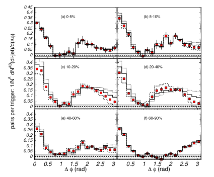
Bottom: The PHENIX analysis[65] shows jet-splitting for sufficiently central events. Reprinted figure 2 with permission from S. S. Adler et al., Phys. Rev. Lett. 97, 052301 (2006), http://link.aps.org/abstract/PRL/v97/p052301. Copyright 2006 by the American Physical Society.
In reference to the images in this figure, we note in accord with the publisher’s guidelines that “Readers may view, browse, and/or download material for temporary copying purposes only, provided these uses are for noncommercial personal purposes. Except as provided by law, this material may not be further reproduced, distributed, transmitted, modified, adapted, performed, displayed, published, or sold in whole or part, without prior written permission from the American Physical Society.”
The PHENIX analysis[65] is similar to the STAR analysis,[64] but with more restrictive cuts: in particular, the less energetic hadron was required to have transverse momentum greater than . The resulting histograms, with a zero-yield-at-minimum (ZYAM) subtraction, show a distinct minimum in associated hadron production at , with a broad maximum in the ballpark of . This jet-splitting persists down to roughly centrality, meaning that it occurs for events where the impact parameter is less than about . The ZYAM subtraction is an important part of the analysis, especially for the less central events. The reason a subtraction is needed is that for a non-central collision, there is an angular modulation of single-particle yields, approximately proportional to , where the zero of coincides with the azimuthal direction of the impact parameter, and the elliptic flow coefficient depends on the transverse momentum and species. Two-point hadron correlators receive a contribution from single-hadron yields. The ZYAM scheme is to subtract a multiple of the appropriate product of single-particle yields. The multiple is chosen so that the resulting histogram has one bin with zero net events, while all other bins have a positive net number of events.
A natural hypothesis is that the high-angle emission leading to either jet-splitting or jet-broadening can be described in terms of a sonic boom in the medium.[70, 71] Two related difficulties afflict this idea. First, it’s hard to get a sonic boom with a big enough amplitude to account for the data[65] with reasonable rates of energy loss;[72, 45] it should be noted however that not all investigators agree on this point,[73] and that there are some phenomenological models based on sonic booms that fit the data.[74, 75] Second, one usually finds a diffusion wake with comparable strength to the sonic boom.[71, 52, 30, 76] At least in a static medium, it is hard to get jet-splitting in the presence of a significant diffusion wake.
To compute the relative strength of the diffusion wake and sonic boom for the heavy quark in the SYM theory, we go back to the conservation equation (99),
| (176) |
In section 6.1.2 we saw that at small , the components of the stress-energy tensor may be decomposed into terms containing sound poles at and terms associated with a wake which have a pole at . If is the leading, small contribution to the stress-energy tensor, then we may decompose
| (177) |
where
| (178) |
and
| (179) |
Since only the terms in (177) contribute to the total drag force in (176), this gives a natural division of the total drag force:
| (180) |
From (124), (125), (126), and (127), we find that
| (181) |
In our conventions, the zero component of gives us the total rate of change in the energy density plus any energy flux going out of the system. Thus, the ratio of energy going into sound waves to energy going into the wake is
| (182) |
While sound modes carry energy away from the moving quark, the wake feeds energy in toward the quark. While this may seem counter-intuitive, in some sense it’s obvious: the diffusion wake consists of a flow of the medium forward toward the quark. The forward-moving momentum in the diffusion wake is the momentum deposited by the quark at earlier times. Qualitatively, (182) says that the diffusion wake and the sonic boom have comparable strength. When comparing (182) to the scenarios of energy loss in the literature,[71, 72] one finds that (182) quantitatively matches a scenario where the relative strength of the wake is so large that it washes out features of jet-splitting associated with the sonic boom. It may be significant, however, that the medium is infinite and static, both in our work and in the linear hydrodynamic scenario[71] that our results match onto at large length scales.
In light of the difficulties in explaining the data with a “boom and wake” model, focused on the hydrodynamic regime, it is natural to investigate the effect on hadron production of the region of the medium close to the moving quark where hydrodynamics is inapplicable. This has been pursued in a series of works,[63, 77, 78, 79, 80, 81, 82, 83] which we briefly summarize in the next few paragraphs. The first idea is to subtract away the leading order Coulombic contribution to . Up to an overall multiplicative rescaling, these are the quantities we denoted and in section 7. The justification for this is that these fields describe the energy of the energetic parton itself, not the energy lost from it. The remaining energy density, which we will denote as , can be split up as . (Note that in contrast to our definitions of and its variants, explicitly includes the contribution from the bath.) The Poynting vector , with the Coulombic contribution subtracted away, is non-zero only because of the presence of the quark. The basic plan is to use the Cooper-Frye algorithm[84] to convert string theory predictions for into a spectrum of hadrons.
The Cooper-Frye algorithm is based on converting a fluid element at temperature and with local four-velocity into hadrons according a Maxwell-Boltzmann distribution in the local rest frame:
| (183) | |||||
where is the number of hadrons, and we have set
| (184) |
and
| (185) |
Note that because of our choice of mostly plus signature, the energy of the hadron in the local rest frame of the fluid is . Also because of this choice of signature, we are obliged to include an explicit minus sign in the first integral expression of (183).
To understand (183)–(185), it helps to refer to figure 8. The momentum of the associated hadron is , and (183) is written in the approximation that the associated hadron is massless—an excellent approximation since a typical hadron of interest is a pion with . The rapidity is related to the angle from the beamline by
| (186) |
(Note that rapidity has nothing to do with the depth coordinate used in previous sections.) The freeze-out surface is chosen to be a slice of constant in (183). This is the best motivated choice for an infinite, asymptotically static medium. In an expanding medium, a more usual choice is a fixed-temperature surface with the temperature set close to the QCD scale. For isochronous freeze-out, the measure is simply , and in passing to the second line of (183) we have simply expressed the metric on in radial coordinates. It is important to realize that the azimuthal angle around the direction of motion of the parton (assumed to be in the direction, as usual) is different from the azimuthal angle around the beamline. We have omitted in (183) a subtraction of the contribution of the bath to hadron production, which depends on but not on . We have also not attempted to normalize : doing so would involve partitioning over the spectrum of hadrons.
The information from string theory enters into (183) in two ways. First, the local four-velocity is the local rest frame of the medium, in which the Poynting vector vanishes. Second, the temperature is the temperature in this local rest frame, deduced by plugging the energy density into the equation of state. Evidently, one needs all components of in order to precisely determine and . This is a problem since only the row of the stress tensor has been computed in full.[52, 53] Another problem is that close to the quark, the medium is presumably far from equilibrium, so using Cooper-Frye seems somewhat perilous. We will return to a discussion of these two issues below.
To understand how hydrodynamical and non-hydrodynamical effects contribute to the spectrum of produced hadrons, one must have some notion of where the boundary is between hydrodynamical and non-hydrodynamical regimes. This boundary is presumably not sharp. Three considerations have gone into identifying an appropriate boundary:
- 1.
The non-hydrodynamical region can be chosen as the region where is less than some constant of order unity. For
(187) a preferred choice is
(188) Here and below, we will describe the region defined by (188) with the parameter choices (187) as the “Neck.” It extends roughly over and . (For , corresponds to .)
- 2.
The Neck region can be compared with the region where the Knudsen number exceeds some constant of order unity. An appropriate version of the Knudsen number in the current context is
(189) Here the sound attenuation length is the same as the one discussed following (120): . For the choice of parameters (187), examination of the near-field expressions (164) shows that the region where is somewhat bigger in the direction than the Neck. However, corrections to the near-field approximation to may not be negligible for and/or of order unity.
- 3.
The Neck region can be compared with the region where the constitutive relations of hydrodynamics break down. Given all components of the stress tensor, with the Coulomb field subtracted away, there is a straightforward procedure for testing the constitutive relations. First determine the local velocity field by passing to the local rest frame of the fluid. Let be the subtracted stress-energy tensor in the local rest frame. The energy density is read off immediately as ; the pressure is deduced from the equation of state; and the shear viscosity contribution to the space-space parts of the stress tensor can be determined from and its gradient. Deviations of the space-space components of from the combined contribution of pressure and shear viscosity are measures of the failure of hydrodynamics.
A study[78] of the near-field expressions (164) for a somewhat different choice of parameters from (187) (namely , , ) concludes that deviations from hydrodynamics are appreciable out as far as . However, the near-field expressions definitely cannot be trusted at such large distances.99 9 A computation of the energy radiated from a moving quark[53] shows that agreement with linearized hydrodynamics is already fairly good at . Based on results of an earlier study,[50] the onset of reasonable agreement with linearized hydro occurs near . This analysis could therefore be considerably improved if all components of were computed directly from string theory.
The main conclusion to draw from points 2 and 3 is that in the Neck region, the subtracted stress tensor is essentially unrelated to hydrodynamics. Instead, the physics may be presumed to be dominated by strong coherent color fields combined with responses of the medium to strong field gradients: hence the term “chromo-viscous neck.”
To return to hadronization: The Cooper-Frye integral over can be split into the Neck region and the “Mach” region—which is everything else. In the Mach region, where the energy density comes mainly from the bath, a good approximation to the local rest frame can be found by setting
| (190) |
In the neck region, this approximation is less reliable, but because space-space components of are not available from a string theory calculation, it is hard to give a better motivated prescription for determining the local rest frame. With the choice (190), the result is that the Neck contribution to the Cooper-Frye integral leads to a distinctive double-peaked structure in for . This is remarkable when compared to the single-peaked structure emerging from a computation in a perturbative QCD framework based on Joule heating,[81] which is similarly passed through the Cooper-Frye hadronization algorithm. See figure 9.

The double-peaked structure from the Neck region of the trailing string stress tensor has nothing to do with the Mach cone. It doesn’t occur at the same angle: for example, at , the Mach angle is very nearly zero, but the Neck region still produces a double peak structure (not shown in figure 9) about a radian away from . When is very close to , the double peaks get closer to . This is reminiscent of the structure observed at large in Fourier space,[54, 46] but the peaks observed in the predicted hadron spectra are more widely separated than the ones in Fourier space.
While the hadronization studies[63, 77, 78, 79, 80, 81, 82, 83] give valuable insight into the relation of the trailing string to high-angle hadron emission from an energetic parton, it is not claimed that the results are fully realistic, or that a direct comparison to untagged dihadron histograms, like the ones in figure 7, is justified. Let us review the potential difficulties. First, the trailing string describes an infinitely massive quark that propagates at a constant velocity through an infinite, static, thermal medium. Fluctuations leading to stochastic motions of finite mass quarks may significantly affect the results. Also, there may be an effective “form factor” for massive quarks that partially smears out the field close to the quark. In addition, it is not obvious that Cooper-Frye is justified, because the crucial effect comes from the non-equilibrium part of the medium (the Neck). Subtracting away the Coulomb field is certainly well-motivated physically, but it is possible to maintain some skepticism about whether it is the correct prescription in combination with Cooper-Frye. Finally, the approximation (190) to the local rest frame is imprecise in the Neck region.
Despite these potentially serious issues, the punchline of the phenomenological studies[63, 77, 78, 79, 80, 81, 82, 83] seems to us likely to be robust: the near-quark region has a substantially greater tendency toward high angle emission in the trailing string treatment than in the perturbative QCD treatment based on Joule heating. Modulo concerns already expressed, the near-field contribution to high-angle emission is stronger than the contribution of the hydrodynamical regime, and it results in a significant double-hump structure, reminiscent of jet-splitting.
9 Conclusions
Let us conclude by addressing the four main questions we raised in the introduction:
- 1.
What is the rate of energy loss from an energetic probe?
For a heavy quark moving at a velocity , the drag force is . This is explained in more detail in section 4.
- 2.
What is the hydrodynamical response far from the energetic probe?
- 3.
What gauge-invariant information can be extracted using the gauge-string duality about the non-hydrodynamic region near the probe?
The expectation values of the energy density and the Poynting vector of the gauge theory stress tensor have been computed with uniformly good accuracy across all length scales for several values of the velocity of the heavy quark, as we review in section 7. Analytic approximations to the space-space components of are also available at small length scales: see section 6.2.
- 4.
Do the rate and pattern of energy loss have some meaningful connection to heavy ion phenomenology?
A suitable translation of parameters from SYM to QCD results in estimates of energy loss for and quarks which are not far from realistic, or which may be fully realistic. We summarize these estimates in section 4.
Studies of hadronization starting from the string theory predictions for the energy density and Poynting vector indicate that the trailing string leads to significant high-angle emission from the Neck region, close to the quark, suggestive of jet-splitting. We describe these studies in section 8. Although it is premature to make detailed comparisons to data, it is clearly worthwhile to extend and refine both the string theory analysis and the phenomenological studies.
Acknowledgments
We thank M. Gyulassy and J. Noronha for useful correspondence. This work was supported in part by the Department of Energy under Grant No. DE-FG02-91ER40671 and by the NSF under award number PHY-0652782. F.D.R. was also supported in part by the FCT grant SFRH/BD/30374/2006.
Appendix A Notation
In this appendix we present short explanations of some of the nomenclature and mathematical notations used in the main text.
- :
The five spacetime coordinates of AdS5-Schwarzschild, usually .
- , :
The four-vectors for position and momentum in . We use mostly plus signature, so (for example) .
- , :
The three-vectors for position and momentum: spatial components of and .
- :
This could mean either or . Our convention is to prefer the latter; likewise and .
- :
The radial distance from the quark in the , plane: . Occasionally we consider the two-vector .
- :
This is the depth coordinate in AdS5 or AdS5-Schwarzschild which is at the boundary and has dimensions of length. The AdS5 metric is .
- :
The depth of the horizon in AdS5-Schwarzschild, related to the temperature by .
- :
Usually, a rescaled depth coordinate in AdS5-Schwarzschild, defined by . But in section 8 we use to denote rapidity, i.e. where is the momentum along the beampipe and is the energy.
- :
We use to indicate a radial separation in . Some authors use to denote the depth coordinate in AdS5.
- AdS5:
Five-dimensional anti-de Sitter space, the maximally symmetric negatively curved spacetime in dimensions. Its metric is given by (3) with .
- SYM:
An abbreviation for “ super-Yang-Mills theory in four dimensions,” which is the theory controlling the low-energy excitations of D3-branes.
- :
Usually, the number of colors: in QCD. An exception is that in section 8, we use to indicate the number of hadrons predicted by the Cooper-Frye algorithm.
- :
The gauge coupling of SYM, normalized so that , where is the number of colors.
- :
The gauge coupling of QCD. We also use .
- :
The ’t Hooft coupling, .
- :
The radius of curvature of AdS5.
- :
The Regge slope parameter of fundamental strings, see (14).
- :
The five-dimensional gravitational coupling.
- :
The spacetime metric of AdS5 or AdS5-Schwarzschild.
- :
The Ricci scalar in AdS5 or AdS5-Schwarzschild. We also use the Ricci tensor and the Riemann tensor . Our conventions are and , with signs arranged so that in AdS5 of radius .
- :
The “blackening function” for AdS5-Schwarzschild, whose metric is given in (3). It is given by . We sometimes think of as a function of the depth , and sometimes as a function of . always means .
- :
The temperature in the dual field theory, which is the same as the Hawking temperature of the dual black hole background. The temperature of the AdS5-Schwarzschild background (3) is .
- :
The worldsheet metric of a string.
- :
Coordinates on the string worldsheet.
- :
The speed of a moving quark. Usually we take this motion to be in the direction.
- :
- :
The embedding function for a classical string in AdS5-Schwarzschild. When no ambiguity is possible, we denote this embedding function more simply as .
- :
The nuclear modification factor, defined as the number of particles produced (usually at a particular value of and in a specified range of rapidity) in a collision of two nuclei with atomic number , divided by the number produced in a proton-proton collision scaled up by the effective number of binary nucleon-nucleon collisions in the heavy-ion collision.
- :
The five-dimensional stress-energy tensor, not to be confused with the expectation value of the boundary stress-energy tensor . For the trailing string, is given in (42).
- :
- :
Small metric perturbations around AdS5-Schwarzschild.
- :
The Fourier components of defined by analogy with (46).
- Axial gauge:
A gauge choice for the metric perturbations where .
- :
The Fourier components of in axial gauge, up to a normalization factor. See (49). We think of the as functions of , not of .
- :
- :
The scalar master field. A master field is a gauge-invariant combination of metric fluctuations in AdS5-Schwarzschild with a simple equation of motion. We encountered four other master fields: , , , and : see (67).
- :
A recurring normalization factor given by .
- :
The momentum conjugate to ; used as a dimensionless wave-number to parameterize the three-dimensional Fourier space used to describe the medium’s response to the quark.
- :
The magnitude of the component of perpendicular to the motion of the quark.
- :
The asymptotic values of at . The boundary condition says that the four-dimensional metric which the boundary gauge theory experiences is flat Minkowski space.
- :
- :
The coefficients of in a small expansion of when . They are related to the expectation value of the boundary stress-energy tensor by (91).
- :
The metric of the boundary conformal field theory, usually set equal to the Minkowski metric with mostly plus signature.
- :
The four-velocity of a heavy quark moving through the thermal medium.
- :
The one-point function of the stress-energy tensor in SYM in the presence of the moving quark. We find it convenient to decompose it into three pieces given in (89).
- :
A stress tensor which satisfies the hydrodynamic constitutive relations, (120). is the hydrodynamic contribution to the stress tensor of the SYM theory.
- :
- :
The source term for the energy-momentum tensor, . Various superscripts specify which contribution of the energy-momentum tensor is being sourced. For example, sources .
- :
The coefficient of the leading homogeneous solution for various linear combinations of and their derivatives, such as , , , , etc. Our boundary condition is .
- :
The analog of for various linear combinations of and their derivatives.
- :
- :
The component of momentum perpendicular to the beamline.
- :
An angular coordinate in momentum space, , or in real space, .
- :
The azimuthal angle around the direction of motion of an energetic quark. Our usual convention is that the energetic quark moves in the direction, and then or .
- :
The angle of a trajectory relative to the beam. is mid-rapidity.
- :
The azimuthal angle around the beam. The angular variable in dihadron histograms is the separation in between two hadrons.
- :
Modified Bessel functions of the first and second kind. is a Bessel function of the first kind, and is a modified Struve function.
- Neck:
The neck is the region near a moving quark where the response of the medium is non-hydrodynamical. In practice, for the choice of parameters (187), the Neck can be defined, as in (188), as the region where the energy density, excluding the Coulombic contribution, exceeds times the asymptotic energy density of an infinite static bath.
- :
The four-velocity of a fluid element, usually defined so that it vanishes in precisely the same Lorentz frame in which the Poynting vector vanishes.
- :
The energy density and Poynting vector, rescaled to make them dimensionless, with contributions from the thermal bath excluded: see (165) and (172). can be decomposed into a sum of contributions from the Coulomb field of the quark, subleading UV effects, IR effects, and a residual quantity , as in (166). An analogous decomposition can be performed on .
References
- [1] J. M. Maldacena, “The large N limit of superconformal field theories and supergravity,” Adv. Theor. Math. Phys. 2 (1998) 231–252, hep-th/9711200.
- [2] S. S. Gubser, I. R. Klebanov, and A. M. Polyakov, “Gauge theory correlators from non-critical string theory,” Phys. Lett. B428 (1998) 105–114, hep-th/9802109.
- [3] E. Witten, “Anti-de Sitter space and holography,” Adv. Theor. Math. Phys. 2 (1998) 253–291, hep-th/9802150.
- [4] S. S. Gubser and A. Karch, “From gauge-string duality to strong interactions: a Pedestrian’s Guide,” 0901.0935.
- [5] O. Aharony, S. S. Gubser, J. M. Maldacena, H. Ooguri, and Y. Oz, “Large N field theories, string theory and gravity,” Phys. Rept. 323 (2000) 183–386, hep-th/9905111.
- [6] I. R. Klebanov, “TASI lectures: Introduction to the AdS/CFT correspondence,” hep-th/0009139.
- [7] E. D’Hoker and D. Z. Freedman, “Supersymmetric gauge theories and the AdS/CFT correspondence,” hep-th/0201253.
- [8] S. S. Gubser, I. R. Klebanov, and A. W. Peet, “Entropy and Temperature of Black 3-Branes,” Phys. Rev. D54 (1996) 3915–3919, hep-th/9602135.
- [9] J. Dai, R. G. Leigh, and J. Polchinski, “New Connections Between String Theories,” Mod. Phys. Lett. A4 (1989) 2073–2083.
- [10] J. Polchinski, “Dirichlet-Branes and Ramond-Ramond Charges,” Phys. Rev. Lett. 75 (1995) 4724–4727, hep-th/9510017.
- [11] E. Witten, “Bound states of strings and p-branes,” Nucl. Phys. B460 (1996) 335–350, hep-th/9510135.
- [12] J. H. Schwarz, “Covariant Field Equations of Chiral N=2 D=10 Supergravity,” Nucl. Phys. B226 (1983) 269.
- [13] G. Policastro, D. T. Son, and A. O. Starinets, “From AdS/CFT correspondence to hydrodynamics,” JHEP 09 (2002) 043, hep-th/0205052.
- [14] S. Bhattacharyya, V. E. Hubeny, S. Minwalla, and M. Rangamani, “Nonlinear Fluid Dynamics from Gravity,” JHEP 02 (2008) 045, 0712.2456.
- [15] G. Policastro, D. T. Son, and A. O. Starinets, “The shear viscosity of strongly coupled N = 4 supersymmetric Yang-Mills plasma,” Phys. Rev. Lett. 87 (2001) 081601, hep-th/0104066.
- [16] S.-J. Rey and J.-T. Yee, “Macroscopic strings as heavy quarks in large N gauge theory and anti-de Sitter supergravity,” Eur. Phys. J. C22 (2001) 379–394, hep-th/9803001.
- [17] C. P. Herzog, A. Karch, P. Kovtun, C. Kozcaz, and L. G. Yaffe, “Energy loss of a heavy quark moving through N = 4 supersymmetric Yang-Mills plasma,” JHEP 07 (2006) 013, hep-th/0605158.
- [18] S. S. Gubser, “Drag force in AdS/CFT,” Phys. Rev. D74 (2006) 126005, hep-th/0605182.
- [19] J. Casalderrey-Solana and D. Teaney, “Heavy quark diffusion in strongly coupled N = 4 Yang Mills,” hep-ph/0605199.
- [20] K. Peeters, J. Sonnenschein, and M. Zamaklar, “Holographic melting and related properties of mesons in a quark gluon plasma,” Phys. Rev. D74 (2006) 106008, hep-th/0606195.
- [21] H. Liu, K. Rajagopal, and U. A. Wiedemann, “An AdS/CFT calculation of screening in a hot wind,” hep-ph/0607062.
- [22] M. Chernicoff, J. A. Garcia, and A. Guijosa, “The energy of a moving quark-antiquark pair in an N = 4 SYM plasma,” hep-th/0607089.
- [23] J. Casalderrey-Solana and D. Teaney, “Transverse momentum broadening of a fast quark in a N = 4 Yang Mills plasma,” JHEP 04 (2007) 039, hep-th/0701123.
- [24] S. S. Gubser, “Momentum fluctuations of heavy quarks in the gauge-string duality,” Nucl. Phys. B790 (2008) 175–199, hep-th/0612143.
- [25] C. P. Herzog, “Energy loss of heavy quarks from asymptotically AdS geometries,” JHEP 09 (2006) 032, hep-th/0605191.
- [26] P. Talavera, “Drag force in a string model dual to large-N QCD,” JHEP 01 (2007) 086, hep-th/0610179.
- [27] E. Caceres and A. Guijosa, “Drag force in charged N = 4 SYM plasma,” JHEP 11 (2006) 077, hep-th/0605235.
- [28] G. Michalogiorgakis, Heavy ion collisions, quasi-normal modes and non-linear sigma models. PhD thesis, Princeton University, 2007.
- [29] C. P. Herzog and A. Vuorinen, “Spinning Dragging Strings,” JHEP 10 (2007) 087, 0708.0609.
- [30] S. S. Gubser and A. Yarom, “Universality of the diffusion wake in the gauge-string duality,” Phys. Rev. D77 (2008) 066007, 0709.1089.
- [31] M. Chernicoff and A. Guijosa, “Acceleration, Energy Loss and Screening in Strongly-Coupled Gauge Theories,” JHEP 06 (2008) 005, 0803.3070.
- [32] Y. Hatta, E. Iancu, and A. H. Mueller, “Jet evolution in the N=4 SYM plasma at strong coupling,” JHEP 05 (2008) 037, 0803.2481.
- [33] Y. Akamatsu, T. Hatsuda, and T. Hirano, “Heavy Quark Diffusion with Relativistic Langevin Dynamics in the Quark-Gluon Fluid,” 0809.1499.
- [34] S. S. Gubser, “Comparing the drag force on heavy quarks in N = 4 super- Yang-Mills theory and QCD,” hep-th/0611272.
- [35] H. Liu, K. Rajagopal, and U. A. Wiedemann, “Calculating the jet quenching parameter from AdS/CFT,” hep-ph/0605178.
- [36] F. Karsch, “Lattice QCD at high temperature and density,” Lect. Notes Phys. 583 (2002) 209–249, hep-lat/0106019.
- [37] D. Bak, A. Karch, and L. G. Yaffe, “Debye screening in strongly coupled N=4 supersymmetric Yang-Mills plasma,” JHEP 08 (2007) 049, 0705.0994.
- [38] O. Kaczmarek and F. Zantow, “Static quark anti-quark interactions in zero and finite temperature QCD. I: Heavy quark free energies, running coupling and quarkonium binding,” Phys. Rev. D71 (2005) 114510, hep-lat/0503017.
- [39] PHENIX Collaboration, A. Adare et. al., “Energy Loss and Flow of Heavy Quarks in Au+Au Collisions at ,” Phys. Rev. Lett. 98 (2007) 172301, nucl-ex/0611018.
- [40] H. van Hees, V. Greco, and R. Rapp, “Heavy-quark probes of the quark-gluon plasma at RHIC,” Phys. Rev. C73 (2006) 034913, nucl-th/0508055.
- [41] H. van Hees and R. Rapp, “Thermalization of heavy quarks in the quark-gluon plasma,” Phys. Rev. C71 (2005) 034907, nucl-th/0412015.
- [42] STAR Collaboration, B. I. Abelev et. al., “Transverse momentum and centrality dependence of high-pt non-photonic electron suppression in Au+Au collisions at ,” Phys. Rev. Lett. 98 (2007) 192301, nucl-ex/0607012.
- [43] J. de Boer, V. E. Hubeny, M. Rangamani, and M. Shigemori, “Brownian motion in AdS/CFT,” 0812.5112.
- [44] W. A. Horowitz and M. Gyulassy, “Testing AdS/CFT Deviations from pQCD Heavy Quark Energy Loss with Pb+Pb at LHC,” 0706.2336.
- [45] J. Casalderrey-Solana, E. V. Shuryak, and D. Teaney, “Hydrodynamic flow from fast particles,” hep-ph/0602183.
- [46] J. J. Friess, S. S. Gubser, G. Michalogiorgakis, and S. S. Pufu, “The stress tensor of a quark moving through N = 4 thermal plasma,” Phys. Rev. D75 (2007) 106003, hep-th/0607022.
- [47] S. S. Gubser and S. S. Pufu, “Master field treatment of metric perturbations sourced by the trailing string,” Nucl. Phys. B790 (2008) 42–71, hep-th/0703090.
- [48] S. S. Gubser, S. S. Pufu, and A. Yarom, “Shock waves from heavy-quark mesons in AdS/CFT,” JHEP 07 (2008) 108, 0711.1415.
- [49] A. Yarom, “On the energy deposited by a quark moving in an N=4 SYM plasma,” Phys. Rev. D75 (2007) 105023, hep-th/0703095.
- [50] S. S. Gubser, S. S. Pufu, and A. Yarom, “Energy disturbances due to a moving quark from gauge-string duality,” JHEP 09 (2007) 108, 0706.0213.
- [51] P. M. Chesler and L. G. Yaffe, “The wake of a quark moving through a strongly-coupled supersymmetric Yang-Mills plasma,” Phys. Rev. Lett. 99 (2007) 152001, 0706.0368.
- [52] S. S. Gubser, S. S. Pufu, and A. Yarom, “Sonic booms and diffusion wakes generated by a heavy quark in thermal AdS/CFT,” Phys. Rev. Lett. 100 (2008) 012301, 0706.4307.
- [53] P. M. Chesler and L. G. Yaffe, “The stress-energy tensor of a quark moving through a strongly-coupled N=4 supersymmetric Yang-Mills plasma: comparing hydrodynamics and AdS/CFT,” Phys. Rev. D78 (2008) 045013, 0712.0050.
- [54] J. J. Friess, S. S. Gubser, and G. Michalogiorgakis, “Dissipation from a heavy quark moving through N = 4 super-Yang-Mills plasma,” JHEP 09 (2006) 072, hep-th/0605292.
- [55] Y.-h. Gao, W.-s. Xu, and D.-f. Zeng, “Wake of color fields in charged N = 4 SYM plasmas,” hep-th/0606266.
- [56] J. Martinez-Morales, “Eigentensors of the Lichnerowicz operator in Euclidean Schwarzschild metrics,” Annalen der Physik 15 (2006), no. 9 653–662.
- [57] P. K. Kovtun and A. O. Starinets, “Quasinormal modes and holography,” Phys. Rev. D72 (2005) 086009, hep-th/0506184.
- [58] V. Balasubramanian and P. Kraus, “A stress tensor for anti-de Sitter gravity,” Commun. Math. Phys. 208 (1999) 413–428, hep-th/9902121.
- [59] S. de Haro, S. N. Solodukhin, and K. Skenderis, “Holographic reconstruction of spacetime and renormalization in the AdS/CFT correspondence,” Commun. Math. Phys. 217 (2001) 595–622, hep-th/0002230.
- [60] S. S. Gubser and A. Yarom, “Linearized hydrodynamics from probe-sources in the gauge-string duality,” 0803.0081.
- [61] I. S. Gradshteyn and I. M. Ryzhik, Table of Integrals, Series, and Products. Academic Press, 7 ed., 2007. Edited by A. Jeffrey and D. Zwillinger.
- [62] A. Yarom, “The high momentum behavior of a quark wake,” Phys. Rev. D75 (2007) 125010, hep-th/0702164.
- [63] J. Noronha, G. Torrieri, and M. Gyulassy, “Near Zone Navier-Stokes Analysis of Heavy Quark Jet Quenching in an =4 SYM Plasma,” Phys. Rev. C78 (2008) 024903, 0712.1053.
- [64] STAR Collaboration, J. Adams et. al., “Distributions of charged hadrons associated with high transverse momentum particles in p p and Au + Au collisions at s(NN)**(1/2) = 200-GeV,” Phys. Rev. Lett. 95 (2005) 152301, nucl-ex/0501016.
- [65] PHENIX Collaboration, S. S. Adler et. al., “Modifications to di-jet hadron pair correlations in Au + Au collisions at s(NN)**(1/2) = 200-GeV,” Phys. Rev. Lett. 97 (2006) 052301, nucl-ex/0507004.
- [66] PHENIX Collaboration, A. Adare et. al., “Dihadron azimuthal correlations in Au+Au collisions at ,” Phys. Rev. C78 (2008) 014901, 0801.4545.
- [67] J. G. Ulery, “Two- and Three-Particle Jet-Like Correlations,” 0801.4904.
- [68] STAR Collaboration, B. I. Abelev et. al., “Indications of Conical Emission of Charged Hadrons at RHIC,” 0805.0622.
- [69] J. G. Ulery, “Conical Emission in Heavy Ion Collisions,” J. Phys. G35 (2008) 104032, 0807.1613.
- [70] H. Stoecker, “Collective Flow signals the Quark Gluon Plasma,” Nucl. Phys. A750 (2005) 121–147, nucl-th/0406018.
- [71] J. Casalderrey-Solana, E. V. Shuryak, and D. Teaney, “Conical flow induced by quenched QCD jets,” J. Phys. Conf. Ser. 27 (2005) 22–31, hep-ph/0411315.
- [72] A. K. Chaudhuri and U. Heinz, “Effect of jet quenching on the hydrodynamical evolution of QGP,” Phys. Rev. Lett. 97 (2006) 062301, nucl-th/0503028.
- [73] J. Casalderrey-Solana and E. V. Shuryak, “Conical flow in a medium with variable speed of sound,” hep-ph/0511263.
- [74] T. Renk and J. Ruppert, “Mach cones in an evolving medium,” Phys. Rev. C73 (2006) 011901, hep-ph/0509036.
- [75] T. Renk and J. Ruppert, “The rapidity structure of Mach cones and other large angle correlations in heavy-ion collisions,” Phys. Lett. B646 (2007) 19–23, hep-ph/0605330.
- [76] B. Betz et. al., “Universality of the Diffusion Wake from Stopped and Punch- Through Jets in Heavy-Ion Collisions,” 0812.4401.
- [77] J. Noronha and M. Gyulassy, “Mach-like Angular Correlations Arise Only From the Head Zone of AdS/CFT String Jets,” 0806.4374.
- [78] J. Noronha, M. Gyulassy, and G. Torrieri, “Near Zone Hydrodynamics of AdS/CFT Jet Wakes,” J. Phys. G35 (2008) 104061, 0806.4665.
- [79] J. Noronha, M. Gyulassy, and G. Torrieri, “Non-Mach Conical Di-Jet Correlations Associated with Heavy Quark Jets in AdS/CFT,” 0807.1038.
- [80] M. Gyulassy, J. Noronha, and G. Torrieri, “Conical Di-jet Correlations from a Chromo-Viscous Neck in AdS/CFT,” 0807.2235.
- [81] B. Betz, M. Gyulassy, J. Noronha, and G. Torrieri, “Anomalous Conical Di-jet Correlations in pQCD vs AdS/CFT,” 0807.4526.
- [82] B. Betz, J. Noronha, M. Gyulassy, and G. Torrieri, “Jet Energy Loss and Mach Cones in pQCD vs. AdS/CFT,” 0812.1905.
- [83] G. Torrieri, B. Betz, J. Noronha, and M. Gyulassy, “Mach cones in heavy ion collisions,” Acta Phys. Polon. B39 (2008) 3281–3308, 0901.0230.
- [84] F. Cooper and G. Frye, “Comment on the Single Particle Distribution in the Hydrodynamic and Statistical Thermodynamic Models of Multiparticle Production,” Phys. Rev. D10 (1974) 186.