Neutrino diagnostics of ultra-high energy cosmic ray protons
Abstract
The energy at which cosmic rays from extra-galactic sources begin to dominate over those from galactic sources is an important open question in astroparticle physics. A natural candidate is the energy at the ‘ankle’ in the approximately power-law energy spectrum which is indicative of a cross-over from a falling galactic component to a flatter extra-galactic component. The transition can occur without such flattening but this requires some degree of conspiracy of the spectral shapes and normalizations of the two components. Nevertheless it has been argued that extra-galactic sources of cosmic ray protons which undergo interactions on the CMB can reproduce the energy spectrum below the ankle if the cross-over energy is as low as the ‘second knee’ in the spectrum. This low cross-over model is constrained by direct measurements by the Pierre Auger Observatory which indicate a heavier composition at these energies. We demonstrate that upper limits on the cosmic diffuse neutrino flux provide a complementary constraint on the proton fraction in ultra-high energy extra-galactic cosmic rays and forthcoming data from IceCube will provide a definitive test of this model.
pacs
98.70.Sa, 95.85.RyI Introduction
The flux of cosmic rays (CRs) falls as an approximate power-law in energy, , with from about 1 GeV up to the ‘knee’ in the spectrum at GeV where it steepens to ; it then steepens further to at GeV (the ‘second knee’) and flattens back to at the ‘ankle’ at GeV [1, 2]. A long-standing open question is the transition point between dominance by galactic and extra-galactic sources in the spectrum of ultra-high energy (UHE) CRs. The transition between the two components ought to be accompanied by the appearance of spectral features, e.g. two power-law contributions would naturally produce a flattening in the spectrum if the harder component dominates at lower energies. Hence, the ankle seems to be a natural candidate for this transition [3, 4, 5] (for discussions see Refs. [6, 7]).
It has been argued however that the cross-over of the two contributions might also happen at lower energies without a corresponding flattening of the spectrum or even at a spectral steepening like the second knee [8]. Such a transition would appear to require considerable fine-tuning of the shape and normalization of the two spectra. It has been argued however that the spectral shape required for the extra-galactic component can develop naturally during the propagation of extra-galactic protons in the cosmic microwave background (CMB) over cosmological distances. At an energy of GeV the energy losses due to pair production and cosmic expansion are roughly equal and thus produce a steepening of an initially featureless power-law injection spectrum. In this model the ankle is formed as a result of the dip due to pair production together with a pile-up of protons below the Greisen-Zatsepin-Kuzmin (GZK) suppression which sets in at about GeV due to pion photoproduction [9, 10].
An obvious test of this ‘dip-transition’ model [8] is whether the flux is indeed proton dominated at energies above GeV [11]. Recent measurements of the elongation rate of UHE CR air showers by the Pierre Auger Observatory [12] indicate however an increasingly heavier composition in the energy range GeV [13], in conflict with this expectation. More elaborate models [14, 15, 16] in which the the extra-galactic CRs have a mixed composition and the cross-over occurs between the second knee and the ankle are consistent with the data [17, 18], but lack the simplicity of the dip-transition model. However, this illustrates that even precision measurements of the chemical composition and spectrum of CRs may not be enough to resolve conclusively just where the galactic-to-extra-galactic transition occurs.
An important clue in resolving this puzzle would be the identification of the CR accelerators themselves. Indeed, the Auger data show a correlation (at C.L.) between the arrival directions of CRs with energy above GeV and active galactic nuclei within Mpc [19, 20]. However, this has only deepened the puzzle, indicating the possible return of a lighter composition beyond GeV, since the primaries appear not to have been deflected significantly by intervening inter-galactic and galactic magnetic fields and therefore are more likely to be protons rather than heavy nuclei. The cosmic ray sources ought also to be emitting other messenger particles that are produced during the acceleration process, in particular gamma rays and neutrinos, and these might provide further constraints. Indeed, it has been observed [21] that certain low cross-over models which require very powerful sources are already marginally excluded by experimental upper bounds on diffuse neutrino fluxes. However, a general exclusion of such models based on neutrino bounds alone has not yet been possible, given the uncertainties inherent in the acceleration mechanism as well as the possible cosmic evolution of the sources.
We update and improve this observation [21] in several respects. The bound on diffuse neutrino fluxes below GeV has improved by a factor of 4 between the AMANDA-B10 [22] and the AMANDA-II [23, 24] measurements and will improve further by an order of magnitude after 1 year of observation with IceCube which is currently under construction at the south Pole [25]. In addition, the hybrid measurements of the Pierre Auger Observatory have reduced the uncertainties in the absolute normalization of the UHE CR flux [26] and these measurements disagree with both the AGASA data [27] and the HiRes data [28, 29], which was used in the earlier analysis [21] (see also Ref. [30]). Furthermore, we will present a method to derive differential upper limits on the proton fraction of UHE CRs from experimental bounds on the diffuse neutrino flux.
The outline of this paper is as follows. We start in Sect. II by deriving the luminosity relation between neutrons and neutrinos in optically and magnetically thin sources. In Sect. III we discuss the Boltzmann equations that govern the propagation of UHE CRs and neutrinos. These results are used in Sect. IV to derive upper limits on the extra-galactic proton contribution to UHE CRs from candidate sources such as blazars. We summarise our findings in Sect. V and provide derivations of the results referred to in the main text in the Appendices.
II Extra-galactic Neutrino Production
Cosmic rays originating in cosmic accelerators will typically be accompanied by gamma-rays and neutrinos. This is a consequence of the inelastic hadronic processes which are involved in their production mechanism [31]. Candidate sources for the highest energy CRs such as blazers or gamma ray bursts are expected to accelerate charged particles by the 1st-order Fermi process or ‘diffusive shock acceleration’ in which they repeatedly scatter off a propagating plasma shock front (see Ref. [32]). (It is also possible that UHE CRs are accelerated by the 2nd-order Fermi process, e.g. in the extended lobes of radio galaxies [33].) For efficient acceleration up to the highest observed energies this process has to be repeated many times hence it is essential that a magnetic field confines the charged particles for sufficiently long in the vicinity of the shock front.
Accelerated electrons and other light charged particles will lose their energy in the magnetic field due to synchroton radiation. The resulting photons provide a target for protons and heavier nuclei to undergo meson photo-production and photo-disintegration, respectively. A neutron produced in this process may escape out of the magnetically confined source before it -decays into a CR proton. To maintain the efficiency of the acceleration mechanism, such interactions need to be much less frequent than the acceleration cycle. Charged and neutral pions decay further into high energy neutrinos and gamma rays which are not confined by the magnetic field and can be emitted from the source.
Here we focus on cosmic proton accelerators. Depending on the relative ambient gas and photon densities, charged pion production may proceed either through inelastic scattering [34], or photopion production predominantly through the resonant process [35]. The subsequent decay chain produces high energy neutrinos with an initial flavor ratio of , which is expected to evolve through oscillations into approximately after propagation over cosmological distances [36].
The relative luminosity of neutrons and neutrinos depends on various details of the source [31]. Since the interaction time scale of protons and neutrons is similar, the relative luminosity of neutrinos will tend to be higher in sources which are optically thick to interactions. The life-time, geometry, bulk motion, and magnetic field of the source limits the maximal energy of the emitted protons [37]. Also important are cooling processes of the muons and pions in the source prior to decay, such as adiabatic losses due to the expansion of the source, inverse Compton scattering, Bethe–Heitler pair production, and synchrotron radiation losses [31].
Our working hypothesis in the following can be expressed in terms of the time scales of and interactions ( and ), the decay lifetimes of neutron, pion and muon (, and ), the cooling time scale of charged particles (), the characteristic cycle time of confinement (), and the total confinement time scale (): () ; () ; () ; () ; () .
Conditions () to () ensure that photopion production of neutrons and subsequent diffusion out of the magnetic confinement region is the dominant process of cosmic proton production in an optically thin source. Conditions () and () permit efficient cosmic ray acceleration with a smooth spectrum across a wide range of energy. Finally, condition () ensures that cooling processes of secondary neutrons, pions, and muons have negligible influence on the energy distribution of the emitted neutrons and neutrinos.


Within this working hypothesis the relative number and energy of the neutrinos and neutrons depend only on the kinematics of photo-hadronic interaction, which implies approximate equipartition of the decaying pion’s energy between the neutrinos and the electron, and the relative radiation density in the source. On average, each proton-photon interaction will produce neutrinos per neutron with relative energy per neutrino, i.e.
| (1) |
In the following, we will consider a (hypothetical) source, where photo-pion interaction proceed exclusively via the resonance with fixed values and [21], and the blazar flaring state model [38] that has been previously discussed in Ref. [39].
For a given photon target spectrum in the source the values of and can be obtained using the SOPHIA Monte Carlo code [40] for photo-nucleon interactions and are shown in Fig. 1 for the adopted blazar spectrum. For a fixed proton energy we sample the scattering angle and photon energy in the center-of-mass frame, weighted by the total cross section and the photon distribution, i.e. the integrand of Eq. (14). These parameters are then input to SOPHIA to generate a interaction and the process is repeated times to derive the average values for the neutrino/neutron number and energy.
The neutrino emissivity of flavor is then given by:
| (2) |
Assuming flavor universality as well as and we arrive at the neutrino source luminosity (per co-moving volume):
| (3) |
Note, that the relation (3) derived for optically thin sources can be regarded as a lower limit on the neutrino luminosity as long as energy-loss processes in the source are negligible. We will illustrate this below for the various conditions of our working hypothesis one by one.
Pion production may also proceed predominantly via inelastic scattering if (cf. ()), in the source. For the process , hadronic event generators indicate an inelasticity where is a final state nucleon [41, 42]. Assuming that 2/3 of the final state pions are charged we estimate that the average energy deposit into neutrinos is about with due to the large multiplicity of secondary pions in inelastic collisions. For a neutron luminosity with (typical for relativistic plasma shocks) this will somewhat increase the neutrino flux relative to the neutrons (cf. Eq. (3)).
If neutrons decay within the source, i.e. (cf. ()), and the sources are optically thick, i.e. (cf. ()), then the neutrino to neutron ratio would also be enhanced due to neutron re-conversion into protons through -decay and interactions, as well as simultaneous production of additional neutrinos. The optical thickness of the source depends on the intensity of the radiation field as well as the characteristic size of the acceleration region. In particular, gamma-ray bursts, possible sources of UHE CRs, are optically thick for proton energies larger than GeV given standard parameters [43, 44] so we do not consider direct neutrino emission from such sources in the following (conservative) analysis.
However, if the target photon field gets too thin so that (cf. ()), then the source would rather accelerate protons to higher energy than emit neutrons through photopion interactions. Whereas this does not change the ratio (3) and our analysis remains conservative, both neutron and neutrino emission become inefficient. This is important for neutrino energies below a few GeV in blazars [39], hence we will not use experimental neutrino bounds below GeV for these candidate sources. However, one can envision cosmic ray sources in which there is substantial leakage of protons from the vicinity of the shock wave, which however remain trapped in the source magnetic field until they interact with the photon background, producing neutrons and neutrinos. Thus, in our general analysis of optically thin sources we extend the energy range down to GeV.
Some care has to be taken if cooling processes of secondary pions and muons in the source environment are in fact important (cf. ()) [31, 45]. Synchrotron radiation, inverse Compton (IC) scattering, Bethe–Heitler (BH) pair production, or adiabatic losses can reduce the energy of pions and muons before decay and hence decrease the neutrino luminosity at high energies. Inverse Compton cooling is the most relevant process for photointeractions of pions and muons [31] and its time scale can be related to the synchrotron loss time via the relative co-moving energy densities of photons and the magnetic field, . Here, we have introduced the equipartition parameter which can exceed 1 in baryon-loaded flows due to the low radiation efficiency of relativistic protons [31]. However, Klein-Nishina corrections at high pion and muon energies reduce the efficiency of IC cooling, which might effectively lead to [45]. Hence, we will estimate the time-scale of secondary particle cooling by .
Synchrotron losses of secondary pions and muons in the background magnetic field are important if their lifetime is larger than the energy loss time , given by11 1 We work throughout in natural Heaviside-Lorentz units with , and .
| (4) |
With muon and pion lifetimes of and , respectively, this translates into a critial energy in the observatory frame
| (5) |
above which our relation between neutron and neutrino luminosities is unreliable.
We use neutrino bounds from AMANDA II [23, 24] and Auger [46], as well as the projected sensitivity of IceCube [47], which extend up to energies of a few GeV (in the observatory frame) and, after red-shifting, correspond to neutrino emission in the source up to energies of about GeV and pion/muon production up to a few GeV (since the neutrinos carry only about 1/4 of the pion/muon energy). Equation (5) shows that cooling processes in blazar jet environments with typical boost factor and G [48, 49] may become important for neutrinos from muon decay only at energies of about GeV. However, it has been shown [39] that typically blazar sources become optically thick at these energies which leads to an increase of the neutrino to proton ratio. In contrast, GRBs typically have a much larger magnetic field of order G and a boost factor of . Hence, cooling of secondaries in GRBs cannot be neglected, but as we have noted already they are not optically thin sources at UHE and we do not therefore consider (direct) neutrino emission from them in the following (conservative) discussion.
The ratio of the observable flux of photo-hadronic neutrinos and CRs today can be calculated from the relation (3) using a set of Boltzmann equations that take into account the interactions with the cosmic photon background and the dilution and red-shift via cosmic expansion. We will discuss these equations and their solutions in the next section.



III Propagation of Cosmic Rays and Neutrinos
For a spatially homogeneous distribution of cosmic sources, emitting UHE particles of type , the co-moving number density is governed by a set of 1-dimensional Boltzmann equations of the form
| (6) |
together with the Friedman-Lemaitre equations describing the cosmic expansion rate as a function of the redshift . Non-relativistic and non-interacting matter obeys the equation . The first and second term in the r.h.s. of Eq. (6) describe continuous energy losses (CEL) due to red-shift and pair production on the cosmic photon backgrounds, respectively. The third and fourth terms describe more general interactions involving particle losses ( anything) with interaction rate , and particle generation of the form .22 2 We will illustrate in Appendix A that CEL processes are an approximate formulation of the process . The last term on the r.h.s. of Eq. (6), , corresponds to the luminosity density per co-moving volume of sources emitting CRs of type . In Appendices A, B and C we provide more details regarding the quantities appearing in Eq. (6).
Note, that the Boltzmann equations (6) do not take into account the deflection of charged CRs during their propagation through inter-galactic and galactic magnetic fields. In fact, if synchrotron radiation during propagation is negligible and the source distribution is homogenous, Eq. (6) provides a good approximation of the spectral evolution even for CRs having small rigidity which suffer large deflections [50]. However, magnetic inhomogeneities on small scales will suppress the spectrum of CRs with Larmor radius where is the characteristic distance between sources. It has been shown that for typical inter-galactic magnetic fields of strength nG and coherence length of Mpc, the diffusive propagation of CR protons will start to affect the spectrum below about GeV if Mpc [51]. Depending on the diffusion regime, this can suppress the proton flux at GeV by a factor of 3 to 100. We will return to this point in the discussion of our results.
We adopt the usual concordance cosmology [2] of a flat universe dominated by a cosmological constant with , the rest being cold dark matter with . The Hubble parameter is given by , normalised to its value today of 70 km s-1 Mpc-1. The time-dependence of the red-shift can be expressed via .
The cosmological evolution of the source density per co-moving volume is parameterized as:
| (7) |
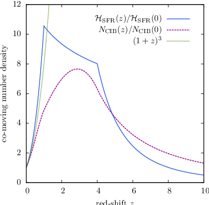
where the source luminosity per co-moving volume is assumed to follow the star formation rate (SFR). (Note that the dilution of the source density due to the Hubble expansion is taken care of since is the comoving density, hence for no evolution we would simply have .) Following the recent compilation [52, 53] we adopt
| (8) |
with appropriate normalization factors, and (see the right panel of Fig. 5).
Some candidate sources of UHE CRs may have a stronger evolution than the star formation rate (8); this is particularly important for cosmogenic neutrinos [54, 55, 56]. For gamma-ray bursts we adopt [54]
| (9) |
Active galactic nuclei may have a similarly strong evolution. Following Refs.[57, 56] we take
| (10) |
with and . We will discuss the impact of these strong evolution scenarios on cosmogenic neutrinos and the proton fraction at very high energies.
In Appendix D we derive a general solution to the differential equation (6). The neutrino flux from the sources is obtained simply by integrating Eqs. (32) and (33):
| (11) |
To obtain the cosmogenic neutrino flux produced during propagation through cosmic radiation backgrounds we need to solve the full Boltzmann equations numerically.
IV Bounds on the Extra-Galactic Proton Fraction
The luminosity relation (3) between neutrinos and CRs in optically thin sources was first used [35] to derive an upper limit on the diffuse neutrino background from UHE CR observations. This argument was modified and extended in further studies which examined if the upper limit on the neutrino flux could in principle be exceeded [58, 21]. With the advent of km3-scale neutrino telescopes like IceCube these limits will soon be tested [21].
As we have outlined in Section II, the relative neutrino luminosity (3) of optically thin sources with photo-hadronic neutrino production (conditions () to ()) can be regarded as a lower limit on the neutrino flux, if cooling processes of secondary pions and muons are negligible () and proton diffusion out of the confinement region is suppressed (). We translate this conservative expectation into an upper limit on the extra-galactic proton fraction in UHE CRs, exploiting experimental upper bounds on the diffuse high-energy neutrino flux.
For this procedure it is convenient to introduce test functions of the neutron source luminosity of the form
| (12) |
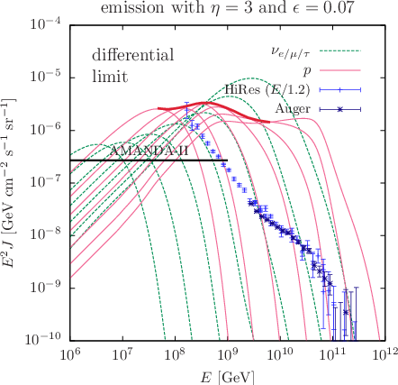
with an exponential energy cut-off that we vary between GeV and GeV with a logarithmic step-size of . Unless otherwise stated, we use Eqs. (7) and (8) for the source evolution. Each neutron test luminosity (12) is related to a neutrino luminosity by the ratio (3). After propagation using Eqs. (6) we normalize the accumulated contribution of extra-galactic and cosmogenic neutrinos to the limit on the diffuse neutrino flux from AMANDA II [23] and to the limit on UHE tau neutrinos from Auger [46]. This can be done in two possible ways.
For an integrated upper limit (or sensitivity) we maximise the individual neutrino flux normalization to saturate the integrated experimental neutrino flux bounds. This approach is shown in the left panels of Fig. 2. The envelope of the corresponding proton flux gives the integrated upper limit on the proton fraction. However, the application of this limit requires that the flux of cosmic neutrinos is close to an spectrum in the quoted interval . Note, that for CR protons above a few times GeV this upper limit becomes trivial, i.e. it lies above the observed CR flux.
A differential upper limit can be obtained using the effective area of AMANDA-II, provided in Ref. [24], and the acceptance () of Auger quoted in Ref. [59]. The normalisation of the neutrino test fluxes is fixed by the integrated limit and the equation
| (13) |
with the appropriate integration limits according to the experimental integrated neutrino flux bound. This second approach is shown in the right panels of Fig. 2. Again, the envelope of the corresponding proton fluxes provides the differential upper limit on the proton fraction. Note, that this differential bound is more general and does not make the usual assumption that the neutrino energy spectrum is , but is in general weaker than the integrated limit by up to a factor of 10.
One year of observation with the fully deployed IceCube detector should increase the sensitivity to diffuse neutrino fluxes by about an order of magnitude below GeV. It is conceivable that this sensitivity can be extended to UHE neutrino energies of about GeV [47]. The corresponding (integrated) sensitivities on the proton fraction in UHE CRs are shown in the upper panels of Fig. 3. We see that 1 year of observation is sufficient to place stringent bounds on the extra-galactic proton fraction in CRs below GeV and thus provide a definitive test of the ‘dip-transition’ model [8].
As noted earlier, the interplay of a random walk of cosmic protons in magnetic fields together with an inhomogenous distribution of their sources may result in suppression of the observed proton flux below about GeV [51]. Hence, we expect that our upper limit on the proton flux in this energy region is rather conservative. In addition, a source evolution much stronger than the star formation rate (8) would predict a much higher flux of neutrinos – cosmogenic as well as from the sources – whereas the spectrum of protons is fixed by the contribution of local sources within the ‘GZK horizon’.
The flux of cosmogenic neutrinos, which dominates the total neutrino flux above GeV, can also in principle be exploited to obtain bounds on the proton fraction independent of the nature of the sources [55]. However, since the CR flux is steeply falling as , to constrain the contribution of trans-GZK protons would require even more sensitive experiments than IceCube and/or a significantly stronger source evolution with redshift than we believe is plausible. In the lower panels of Fig. 3 we estimate the sensitivity of IceCube to constrain the proton fraction using only cosmogenic neutrinos for two strong evolution scenarios (see Eqs. (9) and (10)). Again, the IceCube sensitivity shown to UHE neutrinos up to GeV is extrapolated from lower energies, motivated by the analysis of Ref. [47]. We observe that 1 year of observation at IceCube would be sufficient to constrain trans-GZK protons in UHE CRs only if the source evolution is sufficiently strong: or steeper.

V Conclusions
Exactly where the transition occurs between the galactic and extra-galactic components of UHE cosmic rays is presently an open question and identifying this energy would provide important clues to unravelling their origin. The acceleration of CRs in extra-galactic sources would be accompanied by the emission of high energy neutrinos, thus an upper limit on the proton flux can in principle be inferred from experimental bounds on the extra-galactic UHE neutrino flux. We have demonstrated this, focussing on blazar jets which we have argued are optically thin sources, so photo-hadron interactions generate a certain minimum flux of UHE cosmic neutrinos as long as proton diffusion and secondary particle cooling are negligible. We have shown that this argument is conservative in that a higher neutrino flux would be expected if any of our assumptions are relaxed, e.g. if the sources of UHE CRs are optically thick.
Our main results are summarized in Fig. 4. The AMANDA-II bound on diffuse neutrinos already constrains the extra-galactic proton contribution in CRs at energies below a few times GeV and just 1 year of observation with IceCube will provide the necessary sensitivity up to a few times GeV. If the number density of extra-galactic CR sources evolves strongly with redshift then the detection of cosmogenic neutrinos alone may enable bounds to be placed on the proton flux at trans-GZK energies.
Acknowledgements
MA acknowledges support by STFC UK (PP/D00036X/1). The research of LAA has been partially supported by the US National Science Foundation (Grant PHY-0757598) and UWM’s RGI. SS acknowledges a PPARC Senior Fellowship (PPA/C506205/1) and support from the EU Marie Curie Network “UniverseNet” (HPRN-CT-2006-035863).

Appendix A Photon Background Interactions
The propagation of UHE cosmic nuclei is affected by photo-hadronic interactions on cosmic photon backgrounds. For UHE protons the dominant interactions that determine the spectrum occur on the CMB, but the cosmic infra-red background (CIB) is also important for the generation of cosmogenic neutrinos. For the spectrum of the latter we use the recent compilation of Ref. [60].
The angular-averaged (differential) interaction rate () appearing on the r.h.s. of Eq. (6) is defined as
| (14) | |||
| (15) |
where is the energy distribution of background photons at redshift and is the angular-averaged distribution of particles after interaction. For photo-hadronic interactions this distribution can be determined using the Monte Carlo package SOPHIA [40]. The factor takes into account the relative motion of photons and the nucleus, i.e. the Doppler shift of the photon density.
We assume that the photon background has the adiabatic scaling behaviour:
| (16) |
This is exact for the CMB (following from and ), but not so for the CIB. However, the dominant opacity for proton propagation is provided by the CMB. The scaling behaviour Eq. (16) translates into the following scaling of the quantities and ,
| (17) | ||||
| (18) |
For the adopted scaling of the CIB see Appendix C.
If all interactions can be described as a CEL process the differential equation (33) is considerably simplified and can be solved in a closed form as we will show later. In general, any transition which can be approximated as with can be replaced in the Boltzmann equations (6) as
| (19) |
with . The production of electron-positron pairs in the photon background with a small energy loss is usually approximated as a CEL process. Here we follow the standard approach of Ref. [61] to calculate the proton energy losses in the photon background. Again, the computation of the quantity at various red-shift is significantly simplified if we assume an adiabatically scaling background photon density as for the CMB. The scaling behaviour of and its derivative is then
| (20) | ||||
| (21) |
As before, for the scaling of the infra-red background see Appendix C. In the left panel of Fig. (5) we show the quantities , , and for comparison.
Appendix B Neutron Decay
For neutrons produced by proton interactions on the photon background, the Boltzmann equations have to include a decay term. Since the proton and neutron are much heavier than the electron and electron anti-neutrino we can safely assume that the proton is at rest in the center of mass frame and . The energy distribution of electron and electron anti-neutrino in the nucleon’s rest frame can then be approximated as
| (22) | ||||
| (23) |
according to the phase space density of electron and anti-neutrino with and the constraint . The angular-averaged distribution in the lab frame is
| (24) |
with . The energy of the emerging proton is approximately .


Neutron decay contributes then in the Boltzmann equation in the quantities
| (25) |
for . For neutrons with energy less than GeV the decay length is always smaller than the interaction length in the photon backgrounds (cf. left panel of Fig. 5). In this case it is convenient to approximate the production of neutrons as
| (26) | ||||
| (27) | ||||
| (28) |
We have used this approximation in all our calculations.
Appendix C Evolution of the Infrared-Optical Background
The CIB spectrum has been studied and tabulated in Ref. [60] for red-shifts up to . The red-shift dependence is given by
| (29) |
where is the co-moving luminosity density of the sources and we neglect absorption effects other than expansion. We assume that this follows the star formation rate: . We can then derive the bolometric evolution as
| (30) |
where is the number of infrared–optical photons per proper volume at red-shift . For comparison, the CMB evolves as . To simplify the numerical evaluation we approximate the evolution with redshift as
| (31) |
The redshift scaling of the quantities , , and for the CIB is then obtained from the corresponding scaling given for the CMB in Eqs. (17/18) and (20/21), by multiplying the r.h.s. by a factor . The evolution of the CIB photon number density is shown in the right panel of Fig. 5.
Appendix D Solution of the Boltzmann Equations
We can express the system of partial integro-differential equations (6) in terms of a system of ordinary integro-differential equations,
| (32) | ||||
| (33) |
where we have defined and . The quantity gives the energy that a particle of type had at redshift if we observe it today with energy and take into account CEL. The effective source term in Eq. (33) is
| (34) |
where and are subject to the boundary conditions and . The flux of CRs or neutrinos at can be expressed as
| (35) |
In our calculation we use a logarithmic bin-size of the proton and neutrino energies with between GeV and GeV. For the numerical evolution of the differential equations (32) and (33) we choose a step-size from 0 to 8. The corresponding step-size in the propagation distance is then always smaller than the proton interaction length. In Fig. 6 we compare our results to previous calculations of cosmic proton and cosmogenic neutrino spectra, adopting the same values of the Hubble parameter, source evolution and distribution and the form of the injection spectrum. The agreement is satisfactory in all cases.
References
- [1] M. Nagano and A. A. Watson, Rev. Mod. Phys. 72, 689 (2000).
- [2] C. Amsler et al. [Particle Data Group], Phys. Lett. B 667, 1 (2008).
- [3] J. Linsley, Proceedings of ICRC 1963, Jaipur, India, pp. 77-99
- [4] C. T. Hill and D. N. Schramm, Phys. Rev. D 31, 564 (1985).
- [5] T. Wibig and A. W. Wolfendale, J. Phys. G 31, 255 (2005).
- [6] A. M. Hillas, Nucl. Phys. Proc. Suppl. 136, 139 (2004).
- [7] T. Stanev, Nucl. Phys. Proc. Suppl. 168, 252 (2007).
- [8] V. Berezinsky, A. Z. Gazizov and S. I. Grigorieva, Phys. Rev. D 74, 043005 (2006).
- [9] K. Greisen, Phys. Rev. Lett. 16, 748 (1966).
- [10] G. T. Zatsepin and V. A. Kuzmin, JETP Lett. 4, 78 (1966).
- [11] R. Aloisio, V. Berezinsky, P. Blasi and S. Ostapchenko, Phys. Rev. D 77, 025007 (2008).
- [12] J. Abraham et al. [Pierre Auger Collaboration], Nucl. Instrum. Meth. A 523, 50 (2004).
- [13] M. Unger [for the Pierre Auger Collaboration], Presented at ICRC 2007, Merida, Yucatan, Mexico, 3-11 Jul 2007, arXiv:0706.1495 [astro-ph].
- [14] D. Allard, E. Parizot, E. Khan, S. Goriely and A. V. Olinto, Astron. Astrophys. 443, L29 (2005).
- [15] D. Allard, E. Parizot and A. V. Olinto, Astropart. Phys. 27, 61 (2007).
- [16] D. Hooper, S. Sarkar and A. M. Taylor, Astropart. Phys. 27, 199 (2007).
- [17] D. Allard, A. V. Olinto and E. Parizot, Astron. Astrophys. 473, 59 (2007).
- [18] L. A. Anchordoqui, H. Goldberg, D. Hooper, S. Sarkar and A. M. Taylor, Phys. Rev. D 76, 123008 (2007).
- [19] J. Abraham et al. [Pierre Auger Collaboration], Science 318, 938 (2007).
- [20] J. Abraham et al. [Pierre Auger Collaboration], Astropart. Phys. 29, 188 (2008) [Erratum-ibid. 30, 45 (2008)].
- [21] M. Ahlers, L. A. Anchordoqui, H. Goldberg, F. Halzen, A. Ringwald and T. J. Weiler, Phys. Rev. D 72, 023001 (2005).
- [22] M. Ackermann et al. [IceCube Collaboration], Astropart. Phys. 22, 339 (2005).
- [23] M. Ackermann et al. [IceCube Collaboration], Astrophys. J. 675, 1014 (2008).
- [24] L. Gerhardt [for the IceCube Collaboration], Presented at ICRC 2007, Merida, Yucatan, Mexico, 3-11 Jul 2007, arXiv:0711.0353 [astro-ph].
- [25] A. Achterberg et al. [IceCube Collaboration], Astropart. Phys. 26, 155 (2006).
- [26] J. Abraham et al. [Pierre Auger Collaboration], Phys. Rev. Lett. 101, 061101 (2008).
- [27] M. Takeda et al., Astropart. Phys. 19, 447 (2003).
- [28] T. Abu-Zayyad et al. [HiRes Collaboration], Astropart. Phys. 23, 157 (2005).
- [29] R. Abbasi et al. [HiRes Collaboration], Phys. Rev. Lett. 100, 101101 (2008).
- [30] M. Ahlers, DESY-Thesis-2007-002.
- [31] J. P. Rachen and P. Mészáros, Phys. Rev. D 58, 123005 (1998).
- [32] L. O. Drury, Rept. Prog. Phys. 46, 973 (1983).
- [33] F. Fraschetti and F. Melia, arXiv:0809.3686 [astro-ph].
- [34] L. A. Anchordoqui, H. Goldberg, F. Halzen and T. J. Weiler, Phys. Lett. B 600, 202 (2004).
- [35] E. Waxman and J. N. Bahcall, Phys. Rev. D 59, 023002 (1999).
- [36] J. G. Learned and S. Pakvasa, Astropart. Phys. 3, 267 (1995).
- [37] A. M. Hillas, Ann. Rev. Astron. Astrophys. 22, 425 (1984).
- [38] M. Böttcher, Astrophys. J. 515, L21 (1999).
- [39] L. A. Anchordoqui, D. Hooper, S. Sarkar and A. M. Taylor, Astropart. Phys. 29, 1 (2008).
- [40] A. Mücke, R. Engel, J. P. Rachen, R. J. Protheroe and T. Stanev, Comput. Phys. Commun. 124, 290 (2000). (We have corrected an insignificant error in the sign convention of in eventgen.f pointed out by the authors on the SOPHIA webpage.)
- [41] J. Alvarez-Muniz, R. Engel, T. K. Gaisser, J. A. Ortiz and T. Stanev, Phys. Rev. D 66, 033011 (2002).
- [42] S. R. Kelner, F. A. Aharonian and V. V. Bugayov, Phys. Rev. D 74, 034018 (2006) [Erratum-ibid. D 79, 039901 (2009)].
- [43] T. Piran, Phys. Rept. 314, 575 (1999).
- [44] P. Mészáros, Rept. Prog. Phys. 69, 2259 (2006).
- [45] P. Lipari, M. Lusignoli and D. Meloni, Phys. Rev. D 75, 123005 (2007).
- [46] J. Abraham et al. [Pierre Auger Collaboration], Phys. Rev. Lett. 100, 211101 (2008).
- [47] F. Halzen and D. Hooper, Phys. Rev. Lett. 97, 099901 (2006).
- [48] P. L. Biermann and P. A. Strittmatter, Astrophys. J. 322, 643 (1987).
- [49] L. A. Anchordoqui and H. Goldberg, Phys. Rev. D 65, 021302 (2002).
- [50] R. Aloisio and V. Berezinsky, Astrophys. J. 612, 900 (2004).
- [51] R. Aloisio and V. S. Berezinsky, Astrophys. J. 625, 249 (2005).
- [52] A. M. Hopkins and J. F. Beacom, Astrophys. J. 651, 142 (2006).
- [53] H. Yüksel, M. D. Kistler, J. F. Beacom and A. M. Hopkins, Astrophys. J. 683, L5 (2008).
- [54] H. Yüksel and M. D. Kistler, Phys. Rev. D 75, 083004 (2007).
- [55] H. Takami, K. Murase, S. Nagataki and K. Sato, Astropart. Phys. 31, 201 (2009) [arXiv:0704.0979 [astro-ph]].
- [56] T. Stanev, [arXiv:0808.1045 [astro-ph]].
- [57] G. Hasinger, T. Miyaji and M. Schmidt, Astron. Astrophys. 441, 417 (2005).
- [58] K. Mannheim, R. J. Protheroe and J. P. Rachen, Phys. Rev. D 63, 023003 (2001).
- [59] O. Blanch Bigas [for the Pierre Auger Collaboration], Presented at ICRC 2007, Merida, Yucatan, Mexico, 3-11 July 2007, [arXiv:0706.1658 [astro-ph]].
- [60] A. Franceschini, G. Rodighiero and M. Vaccari, Astron. Astrophys. 487, 837 (2008).
- [61] G. R. Blumenthal, Phys. Rev. D 1, 1596 (1970).
- [62] D. De Marco and T. Stanev, Phys. Rev. D 72, 081301 (2005).
- [63] Z. Fodor, S. D. Katz, A. Ringwald and H. Tu, JCAP 0311, 015 (2003).
- [64] R. Engel, D. Seckel and T. Stanev, Phys. Rev. D 64, 093010 (2001).