A new scheme for the running coupling constant in gauge theories using Wilson loops

One of the key subjects upon which recent attention has been focused is the flavor dependence of $SU(N)$ Yang-Mills theories. In particular, given a number of flavors $N_{f}$, the question is whether the theory has an (approximate) infrared fixed point. This question is triggered by efforts to construct an alternative mechanism of electroweak symmetry breaking, via assuming the existence of a new, strongly interacting sector beyond the electroweak scale [1]. The earliest model of this sort, the so-called technicolor[2, 3], gives rise to a dynamical electroweak symmetry breaking by introducing a QCD-like sector scaled up to some TeV. While theoretically appealing, the simplest form of the technicolor model and its variants with QCD-like dynamics are ruled out or disfavored by electroweak precision measurements. However, the possibility of such mechanism with a non-QCD-like theory [4, 5, 6, 7, 8, 9] is still open, and may provide observable signatures at the LHC. It is thus an important but challenging task to investigate the low-energy landscape of spontaneously broken, strongly interacting gauge theories [10].

Among the theoretical tools at hand, the numerical approach to lattice gauge theories has made it possible to gain quantitative information about strong dynamics of gauge theories. The current understanding can be summarized as follows. A vector-like gauge theory, e.g. QCD, is known to exhibit confinement and dynamical chiral symmetry breaking for small number of massless fermions, $N_{f}$, in the fundamental representation of the gauge group. When $N_{f}$ is just below the value $N_{f}^{af}$ at which the asymptotic freedom sets in, the theory is conformal (unbroken chiral symmetry, no confinement) in the infrared. Such a theory is believed to remain conformal down to some critical value $N_{f}^{c}$, where the coupling becomes strong enough and the transition to the confined chirally broken phase occurs. The range $N_{f}^{c}\leq N_{f}\leq N_{f}^{af}$ is called the conformal window.

It is thus essential to investigate strongly interacting gauge theories in a wide range of parameters, such as the number of colors, the number of flavors, and the fermion representations [11]. Several modern lattice studies in this research direction have recently been performed [12, 13, 14, 15, 16, 17, 18, 19, 20, 21, 22, 23, 24]. In particular, the authors of Refs. [13, 23] performed calculation of the running coupling constant using the Schrödinger functional scheme, and found evidence for an infrared fixed point in $SU(3)$ gauge theory with $N_{f}=12$. However, it is important to study the running coupling constant in different renormalization schemes, in order to conclude that the fixed point is not an artifact due to a particular renormalization prescription but a physical one. For this purpose, we propose a new renormalization scheme which uses the Wilson loops as a key ingredient. Such a scheme is applicable to general gauge theories as long as the Wilson loops can be defined, and provides an efficient computational method for lattice gauge theories. Specifically, a renormalized amplitude is defined as the ratio among the Wilson loops, namely the Creutz ratio, and its perturbative counterpart. The former can be evaluated non-perturbatively by Monte Carlo simulation, while the latter calculated analytically once the underlying theory is specified. By properly defining the non-perturbatively renormalized coupling constant, its scale dependence is extracted using the step-scaling procedure, i.e., from the volume dependence of the coupling [25].

Applying our scheme will provide not only an independent check on the extent of the conformal window, but also several computational advantages. The Creutz ratio can be obtained without $O(a)$ discretization errors, provided these errors are absent in the lattice action. This means our scheme is in principle free from any $O(a)$ systematic effect. Furthermore, this scheme only involves simple gluonic observables, therefore does not introduce any particular kinematical setup which can deteriorate the discretization error or break chiral symmetry. Therefore it can be applied to simulations with dynamical fermions of any type, without restrictions on $N_{f}$. For these features, this scheme may be an attractive alternative to the Schrödinger functional scheme or the twisted Polyakov loop scheme[26, 27, 28].

Before performing calculations for the gauge theories with dynamical fermions, as a benchmark test, we apply this new scheme to the computation of the running coupling constant in quenched lattice QCD. The numerical calculation is performed using the plaquette gauge action with periodic boundary conditions. These boundary conditions are chosen for simplicity. Nevertheless, it results in effects of degenerate vacua known as the “toron” [29]. Our scheme can, however, be applied in principle to any choice of boundary conditions, such as twisted boundary conditions, which ensure no unwanted zero-mode contributions by inducing non-trivial background configurations. Adopting several methods to improve statistical accuracy, we can determine the running of the coupling constant in a wide range of energy scales with a relatively small number of gauge configurations.

Another essential ingredient of our scheme is the perturbative calculation of the renormalization constant. This is performed analytically using zeta function resummation techniques, which prove to be quite convenient. First of all, zeta function techniques offer a natural method to study the analyticity (and regularity) properties of the perturbative counterpart of the Creutz ratio. In addition, some algebraic rearrangements of zeta functions, originally due to Chowla and Selberg [30], allow us to recast the expressions in terms of analytic functions accompanied by some exponentially converging series, whose evaluation is almost trivial and requires little computer power. The zeta function methods we apply can be easily extended to any boundary conditions and to the case of the Polyakov lines [31].

This paper is organized as follows. In the next section we give the definition of the new scheme. The perturbative calculation is illustrated in Sec. 3. Section 4 is devoted to the details of our numerical simulations, after brief introduction to the step-scaling procedure. Section 5 contains discussion on the numerical results and comparison with other results in the literature. Finally, Sec. 6 summarizes our conclusions. The paper contains two appendices where technical details and simulation parameters are reported. Preliminary results of this work have been presented in Ref. [32]

In this section, we define a new renormalization scheme, the ‘Wilson loop scheme’. Let us consider an amplitude ${\cal A}$ whose tree-level approximation is

$${\cal A}^{\rm tree}=kg_{0}^{2}~,$$

(1)

where $g_{0}$ is the bare coupling constant, and $k$ is a coefficient of proportionality that does not depend on $g_{0}$ and can be explicitly calculated for a given underlying theory. With a non-perturbatively calculated amplitude ${\cal A}^{NP}$ at the scale $\mu$, the renormalization constant $Z(\mu)\equiv{\cal A}^{NP}(\mu)/{\cal A}^{\rm tree}$ relates the renormalized coupling constant, $g(\mu)$, to the bare one, leading to the relation

$$g^{2}(\mu)=\frac{{\cal A}^{\rm NP}(\mu)}{k}~.$$

(2)

Although in particle physics an $S$-matrix element, i.e. a scattering amplitude, is usually adopted as ${\cal A}$, to define $g(\mu)$ one can equivalently use any physical quantity that can be perturbatively expanded and is proportional to $g_{0}^{2}$ at the tree-level.

We define the Wilson loop scheme by taking the ‘amplitude’ to be

$${\cal A}_{W}(R;L_{0};g_{0})\equiv-R^{2}\frac{\partial^{2}}{\partial R\partial T}\ln\left.\langle W(R,T;L_{0},T_{0})\rangle\right|_{T=R;T_{0}=L_{0}},$$

(3)

where $W(R,T;L_{0},T_{0})$ is the Wilson loop with the temporal and spatial sizes $T$ and $R$, on a lattice of the physical size $L_{0}^{3}\times T_{0}$. In this work, we take $T_{0}$ to be the same as $L_{0}$, and drop it in the argument of the Wilson loop. The scale $L_{0}$ will be identified as the renormalization scale later. On a finite lattice, $W$, and thus ${\cal A}_{W}$, also depend on the lattice spacing $a$ which is determined by the bare coupling $g_{0}$. The dependence of ${\cal A}_{W}$ on $a$ is removed by taking the continuum limit, $a\rightarrow 0$. A pictorial definition of the Wilson loop is shown in Fig. 2.

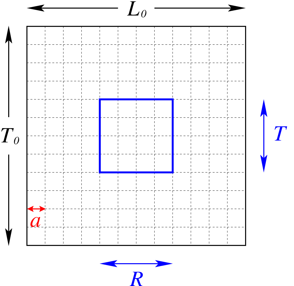
Using lattice perturbation theory (see Fig. 2), ${\cal A}_{W}$ can be shown to be proportional to $g_{0}^{2}$ at the lowest order. Thus, once the value of $k$ is calculated, relation (2) leads to, after taking the continuum limit, a prescription to obtain the renormalized coupling:

$$g^{2}\left(L_{0},\frac{R}{L_{0}}\right)=-{R^{2}\over k(R/L_{0})}{\partial^{2}\over\partial R\partial T}\ln\left.\langle W(R,T;L_{0})\rangle^{\rm NP}\right|_{T=R}.$$

(4)

In the above expression we have made explicit that in the continuum limit $k$ is a regular function of $R/L_{0}$ only. This will be proved in the next section. The remaining factor on the right hand side of Eq. (4) can be evaluated on the lattice as the Creutz ratio,

$$\chi(\hat{R}+1/2;L_{0}/a)=-\left.\ln\left(\frac{W(\hat{R}+1,\hat{T}+1;L_{0}/a)\ W(\hat{R},\hat{T};L_{0}/a)}{W(\hat{R}+1,\hat{T};L_{0}/a)\ W(\hat{R},\hat{T}+1;L_{0}/a)}\right)\right|_{\hat{T}=\hat{R}},$$

(5)

where $\hat{T}\equiv T/a$ and $\hat{R}\equiv R/a$. The value of $\chi$ is evaluated by a Monte Carlo simulation.

The renormalized coupling constant in the Wilson loop scheme can be written as

$$g_{w}^{2}\left(L_{0},\frac{R+a/2}{L_{0}},\frac{a}{L_{0}}\right)=(\hat{R}+1/2)^{2}\cdot\chi(\hat{R}+1/2;L_{0}/a)/k.$$

(6)

The quantity $g_{w}^{2}$ depends on three different scales, $L_{0}$, $R$, and $a$; by taking the ratio to $L_{0}$, we use $r\equiv(R+a/2)/L_{0}$, $a/L_{0}$, and $L_{0}$ as the independent parameters. Fixing $r$ to a specific value means fixing the renormalization scheme. The ratio $a/L_{0}$ specifies the discretization of the box, and can be removed by taking the continuum limit, $a/L_{0}\rightarrow 0$. After fixing the two dimensionless parameters $r$ and $a/L_{0}$, $g_{w}^{2}$ becomes a function of single scale, $L_{0}$. In our scheme, following the step-scaling procedure, $L_{0}$ is identified as the scale at which the renormalized coupling is defined.

Ref. [33] offers an alternative definition of the QCD running coupling related to Wilson loops and discusses its finite-size effects in $L_{0}/R$. Differently from us, their scheme defines the coupling constant in the $\hat{T}\rightarrow\infty$ limit, in which the renormalized coupling is related to the quark force.

There are several advantages in using the Wilson loop scheme. An evident one is that our scheme does not contain $O(a)$ systematic effects as long as they are absent in the lattice action. This is because the Creutz ratio is free from $O(a)$ discretization errors, due to the automatic $O(a)$ improvements of the heavy quark propagator after the redefinition of the mass and the wave function [34]. This is in contrast to the case of the Schrödinger functional scheme, in which the boundary counter terms give rise to additional $O(a)$ systematic errors. Such a particular kinematical setup also breaks chiral symmetry. Furthermore, this scheme only involves simple gluonic observables and can be easily applied to the case with any type of dynamical fermions without restriction to the number of flavors.

One of the indispensable ingredients of the scheme presented in the previous section is the calculation of the coefficient $k$ in Eq. (1). It can be generically split into two terms:

$\displaystyle k=k_{0}+k_{1}~,$

(7)

where $k_{0}$ represents the zero-mode contribution, while $k_{1}$ can be expressed as

$\displaystyle k_{1}=-2\,R^{2}\,C_{F}\,\frac{\partial^{2}}{\partial R\,\partial T}\left[\frac{4}{(2\pi)^{4}}\sum_{n}{}^{{}^{\prime}}\left(\frac{\sin\frac{\pi n_{0}T}{L_{0}}}{n_{0}}\right)^{2}\frac{e^{i\frac{2\pi n_{3}R}{L_{0}}}}{n^{2}}\right]_{T=R}~,$

(8)

where the summation is taken over integer values of $n_{i}$ ($i$=0,…,3) except for the case $n_{0}=n_{1}=n_{2}=n_{3}=0$ (indicated by the prime in the sum), and $n^{2}\equiv n_{0}^{2}+n_{1}^{2}+n_{2}^{2}+n_{3}^{2}$. The zero mode contribution depends on the boundary conditions. In the following, we will concentrate on the case of periodic boundary conditions. In this case, $k_{0}$ was initially calculated in Ref. [29]. For SU$(3)$ gauge group, $k_{0}$ is given by:

$\displaystyle k_{0}=\frac{2}{3}\,C_{F}\left(\frac{R}{L_{0}}\right)^{4}~.$

(9)

The scope of this section is to present a method to compute the quantity $k$. The method we develop will be illustrated for the case of periodic boundary conditions, but it can be applied, with minor changes, to the case of twisted or mixed boundary conditions. As we have seen, the contribution from the zero mode, $k_{0}$, can be separated from the rest and is obviously regular. Thus to compute (and to prove the regularity of) $k$, we only need to consider $k_{1}$. Our starting point is the quantity:

	$\displaystyle S(T/L_{0},R/L_{0})$	$\displaystyle\equiv$	$\displaystyle\sum_{n_{0}=-\infty}^{\infty}{\sin{2\pi T\over L_{0}}n_{0}\over n_{0}}$		(10)
			$\displaystyle\times\left[2\sum_{n_{1},n_{2}}\sum_{n_{3}=1}^{\infty}{\cos{2\pi R\over L_{0}}n_{3}\over n_{0}^{2}+n_{1}^{2}+n_{2}^{2}+n_{3}^{2}}+\sum_{n_{1},n_{2}}^{~~\prime}{1\over n_{0}^{2}+n_{1}^{2}+n_{2}^{2}}\right]~.$

$k_{1}$ can be obtained from $S(T/L_{0},R/L_{0})$ via

$$k_{1}=-{R^{2}C_{F}\over 2\pi^{3}L_{0}}{\partial S\over\partial R}(T/L_{0},R/L_{0})~.$$

Although it is not possible to find a closed form for $S(T/L_{0},R/L_{0})$ in terms of elementary functions, the use of zeta function resummation techniques and basic analytic continuation allows us to recast $S(T/L_{0},R/L_{0})$ into the form of a practically computable quantity, and to prove the regularity of $k$ through an explicit calculation. The computation is carried out in a few steps. The first is the evaluation of the sum over $n_{3}$ by using the Poisson summation formula. Then, the summation over $n_{1}$ and $n_{2}$, is written in terms of the Epstein zeta functions. After these steps, the expression of $S(T/L_{0},R/L_{0})$ becomes compact. However, without further rearrangements, it is of little practical use. To this aim, it is convenient to rewrite the Epstein zeta functions using the Chowla-Selberg formula that renders the zeta functions into the form of elementary analytic functions plus some rapidly converging series. The subsequent step is to analytically perform the integrals introduced when using the Poisson summation formula, and finally perform the remaining summations numerically. Although the above procedure may seem involved, the actual implementation is rather simple. The method has also the bonus of providing a proof of the regularity of the Creutz ratio, as we will explicitly show in the following.

The first step of our procedure is to employ the Poisson summation formula:

$\displaystyle\sum_{n_{3}=1}^{\infty}f(n_{3})=-{1\over 2}f(0)+\int_{0}^{\infty}dtf(t)+2\sum_{n=1}^{\infty}\int_{0}^{\infty}f(t)\cos(2\pi nt)dt~.$

(11)

A straightforward application of the above relation to the function $S(T/L_{0},R/L_{0})$ gives:

$\displaystyle S(T/L_{0},R/L_{0})$

$\displaystyle=$

$\displaystyle 2\sum_{n_{0}=-\infty}^{\infty}{\sin{2\pi T\over L_{0}}n_{0}\over n_{0}}\sum_{m=-\infty}^{\infty}\int_{0}^{\infty}\cos\left(2\pi(m+{R/L_{0}})t\right)\zeta_{t}(s;~n_{0})dt~,$

(12)

where we have used the standard definition of the generalized Epstein zeta function:

$\displaystyle\zeta_{t}(s;n_{0})\equiv\sum_{n_{1}=-\infty}^{\infty}\sum_{n_{2}=-\infty}^{\infty}\left(n_{0}^{2}+n_{1}^{2}+n_{2}^{2}+t^{2}\right)^{-s}~.$

(13)

The parameter $s$ is a regulator, introduced to perform the necessary analytical continuations. The limit $s\rightarrow 1$ will be taken at the end of the calculation. It is interesting that the function $S(T/L_{0},R/L_{0})$ can be entirely written in terms of the integral function

$\displaystyle{\cal Z}(\Omega)$

$\displaystyle=$

$\displaystyle\int_{0}^{\infty}\cos\left(2\pi\Omega t\right)\zeta_{t}(s;n_{0})dt~.$

(14)

Although compact, the result Eq. (12) requires further manipulation. A useful way to handle these functions is to make use of the Chowla-Selberg formula. Refs. [35, 36] develop the appropriate formalism that allows us to express $\zeta_{t}(s;n_{0})$ as the sum of analytic functions plus a rapidly converging series:

	$\displaystyle\zeta_{t}(s;n_{0})$	$\displaystyle=$	$\displaystyle\pi{\Gamma(s-1)\over\Gamma(s)}|n_{0}^{2}+t^{2}|^{(1-s)}+{2\pi\over\Gamma(s)}\sum_{p,q=-\infty}^{\infty~~\prime}\left[\pi^{2}\left({p^{2}}+{q^{2}}\right)\right]^{-(1-s)/2}$		(15)
		$\displaystyle\times$	$\displaystyle\left(n_{0}^{2}+t^{2}\right)^{(1-s)/2}K_{1-s}\left(2\pi\sqrt{n_{0}^{2}+t^{2}}\sqrt{{p^{2}}+{q^{2}}}\right)~.$

The other tool is the following integral formula (see Ref. [37]):

			$\displaystyle\int_{0}^{\infty}\cos\left(2\pi\Omega t\right)\left(t^{2}+n_{0}^{2}\right)^{(1-s)/2}K_{1-s}\left(2\pi(p^{2}+q^{2})^{1/2}(t^{2}+n_{0}^{2})^{1/2}\right)dt$		(16)
		$\displaystyle=$	$\displaystyle\sqrt{\pi\over 2}\left(2\pi\sqrt{p^{2}+q^{2}}\right)^{1-s}n_{0}^{1/2+(1-s)}\left(4\pi^{2}\left(\Omega^{2}+p^{2}+q^{2}\right)\right)^{\frac{s-1}{2}-\frac{1}{4}}$
			$\displaystyle\mbox{ }\mbox{ }\mbox{ }\times K_{(s-1)-1/2}\left(2\pi n_{0}\sqrt{(p^{2}+q^{2})+\Omega^{2}}\right)~.$

The procedure is now straightforward and consists in using the relations (15) and (16) in Eq. (12). Some computations lead to

	$\displaystyle Z(\Omega)$	$\displaystyle=$	$\displaystyle{\sqrt{\pi}\Gamma(2-s)\over\Gamma(s)}2\Gamma(s-1)\cos\left(\pi((1-s)+1/2)\right)\left({n_{0}\over\pi\Omega}\right)^{(1-s)+1/2}K_{(s-1)-1/2}\left(2\pi\Omega n_{0}\right)$		(17)
		$\displaystyle+$	$\displaystyle(2\pi)^{3/2}{2^{-s}\over\Gamma(s)}\sum_{p,q=-\infty}^{\infty~~\prime}n_{0}^{1/2+(1-s)}\left[4\pi^{2}\left({p^{2}}+{q^{2}}+\Omega^{2}\right)\right]^{(s-1)/2-1/4}$
		$\displaystyle\times$	$\displaystyle K_{(s-1)-1/2}\left[2\pi n_{0}\left({p^{2}}+{q^{2}}+\Omega^{2}\right)\right]^{1/2}~.$

It can be easily checked that, in the above expression, the limit $s\rightarrow 1$ can be taken safely giving

$\displaystyle{\cal Z}(\Omega)$

$\displaystyle=$

$\displaystyle{\pi\over 2|\Omega|}e^{-2\pi|\Omega|n_{0}}+{\pi\over 2}\sum_{p,q=-\infty}^{\infty~~\prime}\left({p^{2}}+{q^{2}}+\Omega^{2}\right)^{-1/2}e^{-2\pi n_{0}\sqrt{{p^{2}}+{q^{2}}+\Omega^{2}}}~.$

(18)

It is evident that the quantity ${\cal Z}(\Omega)$ is regular. We can now substitute Eq. (18) into Eq. (10), and rearrange it as

$\displaystyle S(T/L_{0},R/L_{0})$

$\displaystyle=$

$\displaystyle{4\pi^{2}T\over L_{0}}\left[S_{0}(R/L_{0})+S_{1}(T/L_{0},R/L_{0})\right]~,$

(19)

where we have separated the $n_{0}=0$ contribution from the remaining part which is exponentially suppressed. This separation leads to the definition

	$\displaystyle S_{0}(R/L_{0})$	$\displaystyle=$	$\displaystyle A_{1}(R/L_{0})+A_{2}(R/L_{0})+A_{3}(R/L_{0})~,$		(20)
	$\displaystyle S_{1}(T/L_{0},R/L_{0})$	$\displaystyle=$	$\displaystyle B_{1}(T/L_{0},R/L_{0})+B_{2}(T/L_{0},R/L_{0})+B_{3}(T/L_{0},R/L_{0})~,$		(21)

where

	$\displaystyle A_{1}(R/L_{0})$	$\displaystyle\equiv$	$\displaystyle\sum_{m=-\infty}^{+\infty}{1\over 2|m+(R/L_{0})|}~,$		(22)
	$\displaystyle A_{2}(R/L_{0})$	$\displaystyle\equiv$	$\displaystyle 2\sum_{m=-\infty}^{+\infty}\sum_{p,q=1}^{\infty}{1\over\left({p^{2}}+{q^{2}}+|m+(R/L_{0})|^{2}\right)^{1/2}}~,$		(23)
	$\displaystyle A_{3}(R/L_{0})$	$\displaystyle\equiv$	$\displaystyle 2\sum_{m=-\infty}^{+\infty}\sum_{p=1}^{\infty}{1\over\left({p^{2}}+|m+(R/L_{0})|^{2}\right)^{1/2}}~,$		(24)
	$\displaystyle B_{1}(T/L_{0},R/L_{0})$	$\displaystyle\equiv$	$\displaystyle\sum_{n_{0}=1}^{\infty}{\sin{2\pi T\over L_{0}}n_{0}\over\pi n_{0}T/L_{0}}\sum_{m=-\infty}^{+\infty}{e^{-2\pi|m+(R/L_{0})|n_{0}}\over 2|m+(R/L_{0})|}~,$		(25)
	$\displaystyle B_{2}(T/L_{0},R/L_{0})$	$\displaystyle\equiv$	$\displaystyle 2\sum_{n_{0}=1}^{\infty}{\sin{2\pi T\over L_{0}}n_{0}\over\pi n_{0}T/L_{0}}\sum_{m=-\infty}^{+\infty}\sum_{p,q=1}^{\infty}{e^{-2\pi n_{0}\sqrt{{p^{2}}+{q^{2}}+|m+(R/L_{0})|^{2}}}\over\left({p^{2}}+{q^{2}}+|m+(R/L_{0})|^{2}\right)^{1/2}}~,$		(26)
	$\displaystyle B_{3}(T/L_{0},R/L_{0})$	$\displaystyle\equiv$	$\displaystyle 2\sum_{n_{0}=1}^{\infty}{\sin{2\pi T\over L_{0}}n_{0}\over\pi n_{0}T/L_{0}}\sum_{m=-\infty}^{+\infty}\sum_{p=1}^{\infty}{e^{-2\pi n_{0}\sqrt{{p^{2}}+|m+(R/L_{0})|^{2}}}\over\left({p^{2}}+|m+(R/L_{0})|^{2}\right)^{1/2}}~.$		(27)

Due to the exponential suppression, the terms $B_{1}$, $B_{2}$, and $B_{3}$, and thus $S_{1}(T/L_{0},R/L_{0})$, are clearly regular. Therefore, to prove the regularity of $k$, we only have to show that $S_{0}(R/L_{0})$ is also regular. To show that the terms (22), (23), and (24) also lead to a regular expression for $S_{0}(R/L_{0})$ (and to compute them), it requires further manipulations.

The first term, (22), can be computed analytically:

$\displaystyle A_{1}(R/L_{0})={1\over 2}\left[-{L_{0}\over R}-\psi(R/L_{0})+\psi(-R/L_{0})\right]~,$

(28)

where $\psi(x)$ is the Euler psi function [37]. The remaining two terms, $A_{2}$ and $A_{3}$, can be rearranged by performing first the summation over $m$, and then by using the Chowla-Selberg formula. We leave the details in Appendix A, and present the results here:

	$\displaystyle A_{2}(R/L_{0})$	$\displaystyle=$	$\displaystyle 8\sum_{j=1}^{\infty}\cos(2j\pi R/L_{0})K_{0}\left(2j\pi\sqrt{p^{2}+q^{2}}\right)+\mbox{($R$-independent terms)}~,$		(29)
	$\displaystyle A_{3}(R/L_{0})$	$\displaystyle=$	$\displaystyle 8\sum_{q,j=1}^{\infty}\cos(2j\pi R/L_{0})K_{0}\left(2j\pi q\right)+\mbox{($R$-independent terms)}~.$		(30)

Written as above, it is a trivial matter to see that, after taking the derivative of $A_{1}$, $A_{2}$, and $A_{3}$ with respect to $R$, $S_{0}(R/L_{0})$, and thus $k$, is nicely behaved due to the exponential fall-off of the Kelvin functions $K_{\nu}(z)$.

The last step of our procedure consists in evaluating the above expressions. The numerical computation of the sums in Eqs. (25), (26), (27), (29), and (30), does not present any problem due to the exponential suppression. Differentiating with respect to $R$, substituting $T/L_{0}=R/L_{0}$, and combining the results according to Eqs. (8), (9), (10) lead to the result for $k$. Figure 3 shows the dependence of the function $k$ with respect to $R/L_{0}$. Table 1 provides some indicative values for $k$.

In this section, we will describe the details of our numerical simulations. For later use, we define the coupling-squared, $\tilde{g}_{w}^{2}$,

$$\tilde{g}_{w}^{2}\left(\beta,\,r,\,\frac{L_{0}}{a}\right)\equiv kg_{w}^{2}~,$$

(31)

where $r\equiv(R+a/2)/L_{0}$. Note that we express $\tilde{g}_{w}^{2}$ as a function of $\beta$, $r$, and $a/L_{0}$ instead of $L_{0}$, $r$ and $L_{0}/a$. The above redefinition is chosen for convenience, since $\beta$, $r$, and $a/L_{0}$ are the actual input parameters for the simulations.

References

- [1] C. T. Hill and E. H. Simmons, Phys. Rept. 381, 235 (2003); 390, 553(E) (2004).
- [2] S. Weinberg, Phys. Rev. D 13, 974 (1976); ibid. 19, 1277 (1979).
- [3] L. Susskind, Phys. Rev. D20, 2619 (1979).
- [4] B. Holdom, Phys. Lett. B150, 301 (1985).
- [5] K. Yamawaki, M. Bando, and K.-i. Matsumoto, Phys. Rev. Lett. 56, 1335 (1986).
- [6] T. Appelquist, D. Karabali, and L. C. R. Wijewardhana, Phys. Rev. Lett. 57, 957 (1986); T. Appelquist and L. C. R. Wijewardhana, Phys. Rev. D 35, 774 (1987); Phys. Rev. D 36, 568 (1987).
- [7] T. Appelquist, J. Terning, and L. C. R. Wijewardhana, Phys. Rev. Lett. 77, 1214 (1996).
- [8] V. Miransky and K. Yamawaki, Phys. Rev. D 55, 5051 (1997); ibid. 56, E 3768 (1997). See also V. Miransky and P. Fomin, Sov. J. Part. Nucl. 16, 203 (1985).
- [9] T. Appelquist, A. Ratnaweera, J. Terning, and L. C. R. Wijewardhana, Phys. Rev. D58, 105017 (1998).
- [10] An early paper on the phase structure of vectorial gauge theories is T. Banks and A. Zaks, Nucl. Phys. B 196, 189 (1982); see also D. D. Dietrich and F. Sannino, Phys. Rev. D 75, 085018 (2007), for extensive investigation of the conformal window including non-fundamental representation fermions.
- [11] Y. Iwasaki et al., Phys. Rev. Lett. 69, 21 (1992); Phys. Rev. D 69, 014507 (2004); P. Damgaard, U. Heller, A. Krasnitz, and P. Olesen, Phys. Lett. B 400, 169 (1997); R. Mawhinney, Nucl. Phys. B (Proc. Suppl.) 83, 57 (2000), for pioneering lattice studies on the phase structure of the large flavor gauge theories.
- [12] S. Catterall and F. Sannino, Phys. Rev. D76, 034504 (2007).
- [13] T. Appelquist, G. T. Fleming, and E. T. Neil, Phys. Rev. Lett. 100, 171607 (2008).
- [14] L. Del Debbio, A. Patella, and C. Pica, arXiv:0812.0570.
- [15] L. Del Debbio, A. Patella, and C. Pica, arXiv:0805.2058.
- [16] L. Del Debbio, M. T. Frandsen, H. Panagopoulos, and F. Sannino, JHEP 06, 007 (2008).
- [17] S. Catterall, J. Giedt, F. Sannino, and J. Schneible, JHEP 11, 009 (2008).
- [18] T. DeGrand, Y. Shamir, and B. Svetitsky, arXiv:0812.1427.
- [19] Y. Shamir, B. Svetitsky, and T. DeGrand, Phys. Rev. D78, 031502 (2008).
- [20] Z. Fodor et al., arXiv:0809.4888.
- [21] Z. Fodor et al., arXiv:0809.4890.
- [22] A. J. Hietanen, J. Rantaharju, K. Rummukainen, and K. Tuominen, arXiv:0812.1467.
- [23] T. Appelquist, G. T. Fleming, and E. T. Neil, arXiv:0901.3766.
- [24] G. T. Fleming, PoS LATTICE2008, 021 (2008).
- [25] M. Luscher, P. Weisz, and U. Wolff, Nucl. Phys. B359, 221 (1991).
- [26] G. de Divitiis et al., Nucl. Phys. B437, 447 (1995).
- [27] G. M. de Divitiis, R. Frezzotti, M. Guagnelli, and R. Petronzio, Nucl. Phys. B433, 390 (1995).
- [28] G. M. de Divitiis, R. Frezzotti, M. Guagnelli, and R. Petronzio, Nucl. Phys. B422, 382 (1994).
- [29] A. Coste, A. Gonzalez-Arroyo, J. Jurkiewicz, and C. P. Korthals Altes, Nucl. Phys. B262, 67 (1985).
- [30] S. Chowla and A. Selberg, Proc. Natl. Acad. Sci. 35, 371 (1949).
- [31] E. Bilgici, A. Flachi, E. Itou, M. Kurachi, C.-J.D. Lin, H. Matsufuru, H. Ohki, T. Onogi, T. Yamazaki, work in progress.
- [32] E. Bilgici et al., arXiv:0808.2875.
- [33] M. Campostrini, P. Rossi and E. Vicari, Phys. Lett. B 349, 499 (1995).
- [34] S. Necco and R. Sommer, Nucl. Phys. B622, 328 (2002).
- [35] E. Elizalde, Commun. Math. Phys. 198 83 (1998).
- [36] K. Kirsten, J. Math. Phys. 35 459 (1994).
- [37] I. S. Gradshteyn and I. M. Ryzhik, ‘Tables of Integrals, Series, and Products’, Academic Press, VI edition.
- [38] M. Luscher, R. Narayanan, P. Weisz, and U. Wolff, Nucl. Phys. B384, 168 (1992).
- [39] S. Caracciolo et al., Phys. Rev. Lett. 74, 2969 (1995).
- [40] M. Albanese et al., Phys. Lett. B192, 163 (1987).
- [41] S. Capitani, M. Luscher, R. Sommer, and H. Wittig, Nucl. Phys. B544, 669 (1999).
- [42] M. Della Morte et al., Nucl. Phys. B713, 378 (2005).
- [43] M. Guagnelli, R. Sommer, and H. Wittig, Nucl. Phys. B535, 389 (1998).
- [44] G. T. Fleming, hep-lat/0403023.