Cosmological Constraints from the SDSS maxBCG Cluster Catalog
Abstract
We use the abundance and weak lensing mass measurements of the SDSS maxBCG cluster catalog to simultaneously constrain cosmology and the richness–mass relation of the clusters. Assuming a flat CDM cosmology, we find after marginalization over all systematics. In common with previous studies, our error budget is dominated by systematic uncertainties, the primary two being the absolute mass scale of the weak lensing masses of the maxBCG clusters, and uncertainty in the scatter of the richness–mass relation. Our constraints are fully consistent with the WMAP five-year data, and in a joint analysis we find and , an improvement of nearly a factor of two relative to WMAP5 alone. Our results are also in excellent agreement with and comparable in precision to the latest cosmological constraints from X-ray cluster abundances. The remarkable consistency among these results demonstrates that cluster abundance constraints are not only tight but also robust, and highlight the power of optically-selected cluster samples to produce precision constraints on cosmological parameters.
Subject headings
cosmology: observation — cosmological parameters — galaxies: clusters — galaxies: halosI. Introduction
The abundance of galaxy clusters has long been recognized as a powerful tool for constraining cosmological parameters. More specifically, from theoretical considerations (pressschechter74; bondetal91; whiteetal93; shethtormen02, e.g.) one expects the abundance of massive halos to be exponentially sensitive to the amplitude of matter fluctuations. Though some theoretical challenges remain (robertsonetal08; staneketal09, see e.g.), this basic theoretical prediction has been confirmed many times in detailed numerical simulations, and a careful calibration of the abundance of halos as a function of mass for various cosmologies has been performed (jenkinsetal01; warrenetal06; tinkeretal08, see e.g.). Despite these successes, realizing the promise of cluster cosmology has proven difficult. Indeed, a review of observational results from the past several years yields a plethora of studies where typical uncertainties are estimated at the level despite a spread in central values that range from to (vianaliddle96; vianaliddle99; henry91; henry00; pierpaolietal01; borganietal01; seljak02; vianaetal02; schueckeretal03; allenetal03; bahcalletal03; bahcallbode03; henry04; voevodkinvikhlinin04; rozoetal07a; gladdersetal07; rinesetal07).
The discrepancies among the various studies mentioned above is a manifestation of the fundamental problem confronting cluster abundance studies: theoretical predictions tell us how to compute the abundance of halos as a function of mass, but halo masses are not observable. Consequently, we are forced to rely on observable quantities such as X-ray temperature, weak lensing shear, or other such signals, to estimate cluster masses. This reliance on observable mass tracers introduces significant systematic uncertainties in the analysis; indeed, this is typically the dominant source of error (henryetal08, e.g.).
There are two primary ways in which these difficulties can be addressed. One possibility is to reduce these systematic uncertainties through detailed follow-up observations of relatively few clusters, an approach exemplified in the work of vikhlininetal08. The second possibility is to use large cluster samples complemented with statistical properties of the clusters that are sensitive to mass to simultaneously fit for cosmology and the observable–mass relation of the cluster sample in question. Indeed, this is the basic idea behind the so called self-calibration approach, in which one uses the clustering of clusters (schueckeretal03; estradaetal08) and cluster abundance data to derive cosmological constraints with no a-priori knowledge of the observable–mass relation (hu03; majumdaretal04; limahu04; limahu05). There are, however, many other statistical observables that correlate well with mass, such as the cluster–shear correlation function (sheldonetal07), or even counts binned in multiple mass tracers (cunha08). By including such data we can break the degeneracy between cosmology and the observable–mass relation, thereby obtaining tight cosmological constraints while simultaneously fitting the observable–mass relation.
In this work, we derive cosmological constraints from the SDSS maxBCG cluster sample (koesteretal07a) and the statistical weak lensing mass measurement from johnstonetal07. We then compare our result to three state-of-the-art cluster abundance studies of X-ray selected cluster samples (mantzetal08; henryetal08; vikhlininetal08b) and demonstrate that our results are both consistent and competitive with these studies. This is the first time an optically selected catalog with masses estimated in a statistical way has produced constraints that are of comparable accuracy to the more traditional approach.
The paper is organized as follows. Section II presents the data used in our study. Section III describes our analysis, including the likelihood model and priors adopted in this work, and the way in which the analysis was implemented. Section IV presents our main results, while sections V.1, V.2, and V.3 discuss various sources of systematic uncertainties. Section VI.1 compares our results to the most recent results from X-ray selected cluster samples. Section investigates the implications of our results for dark energy, and Section discusses the prospects for improving our cosmological constraints from the maxBCG cluster sample in the future. Section summarizes our main results and conclusions. Unless otherwise stated, all masses in this work are defined using an overdensity relative to the mean matter density of the universe.
II. Data
II.1. MaxBCG Cluster Counts
The maxBCG cluster catalog (koesteretal07a) is an optically selected catalog drawn from 7,398 of DR4+ imaging data of the Sloan Digital Sky Survey (SDSS).11 1 We write DR4+ as the catalog used a few hundred degrees of imaging beyond those released with DR4. The maxBCG algorithm exploits the tight E/S0 ridgeline of galaxies in color-magnitude space to identify spatial overdensities of bright red galaxies. The tightness of the color distribution of cluster galaxies greatly suppresses the projection effects that have plagued optically selected cluster catalogs, and also allows for accurate photometric redshift estimates of the clusters (). MaxBCG clusters are selected such that their photometric redshift estimates are in the range , resulting in a nearly volume-limited catalog. A detailed discussion of the maxBCG cluster finding algorithm can be found in koesteretal07.
We bin the maxBCG cluster sample in nine richness bins spanning the range , corresponding roughly to . Our richness measure is defined as the number of red-sequence galaxies within a scaled radius such that the average galaxy overdensity interior to that radius is times the mean galaxy density of the universe (see koesteretal07a, for further details). The richness bins, and the number of clusters in each bin, are presented in Table 1. There are an additional five clusters with richness . These five clusters have , , , , and , and are properly included in the analysis on an individual basis (see §III.1 for details).
| Richness | No. of Clusters |
|---|---|
| 11-14 | 5167 |
| 14-18 | 2387 |
| 19-23 | 1504 |
| 24-29 | 765 |
| 30-38 | 533 |
| 39-48 | 230 |
| 49-61 | 134 |
| 62-78 | 59 |
| 79-120 | 31 |
Figure 1 shows the cluster counts corresponding to Table 1. Error bars between the various points are correlated. Also shown are the modeled counts from our best-fit model, detailed in Section IV. We show these model counts here for comparison purposes.

II.2. MaxBCG Weak Lensing Masses
Estimates of the mean mass of the maxBCG clusters as a function of richness are obtained through the weak lensing analysis described by sheldonetal07 and johnstonetal07. Briefly, sheldonetal07 binned the maxBCG cluster sample in richness bins as summarized in Table 2. Given a cluster in a specified richness bin, they use all cluster–galaxy pairs with the selected cluster as a lens to estimate the density contrast profile of the cluster. While these individual cluster profiles are very low signal-to-noise, averaging over all clusters within a richness bin allows one to obtain accurate estimates for the mean density contrast profile of maxBCG clusters as a function of richness. The resulting profiles are fit using a halo model formalism to derive mean cluster masses by johnstonetal07. We then correct these masses upward by a factor of due to the expected photometric redshift bias due to the dilution of the lensing signal from galaxies that are in front of the cluster lenses, but whose photometric redshift probability distribution extends past the cluster lens (see mandelbaumetal08, for details). A very similar but independent analysis has also been carried out by mandelbaumetal08b, and we use the comparison between the two independent analysis to set the systematic error uncertainty of the weak lensing mass estimates (rozoetal08a). The final results of the weak lensing analysis summarized above are presented here in Table 2.22 2 The number of clusters in Table 2 is larger than that reported in johnstonetal07 due to masking in the weak lensing measurements. This additional masking does not bias the recovered masses in any way. Figure 2 shows the mean weak lensing masses from Table 2. Also shown are the mean masses computed using the best-fit model detailed in Section IV. The richness binning of the weak lensing mass estimates differs from that of the abundance data because of the larger number of clusters necessary within each richness bin to obtain high S/N weak lensing measurements.
| Richness | No. of Clusters | |
|---|---|---|
| 12-17 | 5651 | 1.298 |
| 18-25 | 2269 | 1.983 |
| 26-40 | 1021 | 3.846 |
| 41-70 | 353 | 5.475 |
| 71+ | 55 | 13.03 |
Note. — Masses listed here are based on those quoted in johnstonetal07, rescaled by the expected photometric redshift bias described in the text, and extrapolated to a matter overdensity from the value quoted in johnstonetal07. The masses have also been rescaled to the cosmology that maximizes our likelihood function, , ).
III. Analysis
We employ a Bayesian approach for deriving cosmological constraints from the maxBCG cluster sample. We use only minimal priors placed on the parameters governing the richness–mass relation, relying instead on the cluster abundance and weak lensing data to simultaneously constrain cosmology and the richness–mass relation of the clusters. Details of the model, parameter priors, and implementation can be found below.
III.1. Likelihood Model
The observable vector for our experiment is comprised of:
- 1.
through : the number of clusters in each of the nine richness bins defined in Table 1.
- 2.
We adopt a Gaussian likelihood model, which is fully specified by the mean and covariance matrix of our observables. Expressions for these quantities as a function of model parameters are specified below. We also multiply this Gaussian likelihood by a term that allows us to properly include the information contained in clusters with richness . In this richness range clusters are very rare and a Gaussian likelihood model is not justified. Instead we adopt a likelihood model where the probability of having a cluster of a particular richness is binary (i.e. a Bernoulli distribution), with
| (1) |
Such a probability distribution is adequate so long as the probability of having two clusters of a given richness is infinitesimally small. Note that given this binary probability distribution, we have that the expectation value of the number of such clusters is simply , and the likelihood is fully specified by the expectation value of our observable. We find that the likelihood of observing the particular richness distribution found for the maxBCG catalog for clusters of richness is
| (2) |

The first product is over all richness and no clusters in them, and the second product is over richness bins which contain one cluster. The subscript reflects the fact that it is the likelihood of the tail of the abundance function. The final likelihood is the product of the Gaussian likelihood described earlier and the likelihood of the abundance function tail. We note that the log-likelihood of the tail simplifies to
| (3) | |||||
An identical result is obtained assuming only Poisson variations in the number of clusters for .
III.2. Expectation Values
To fully specify our likelihood model we need to derive expressions for the mean and variance of our observables. The model adopted in this work is very similar in spirit to that of rozoetal07a, so we present here only a brief overview of the formalism. Interested readers can find a detailed discussion in rozoetal07a.
We begin by considering the expected mean number of clusters in our sample. The number of halos within a redshift bin and within a mass range is given by
| (4) |
where is the halo mass function, is the comoving volume per unit redshift, and and are the mass and redshift binning functions. i.e. if is within the mass bin of interest and zero otherwise, and if is within the redshift bin of interest, but is zero otherwise.
In practice, we observe neither a cluster’s mass nor its true redshift, but are forced to rely on the cluster richness as a mass tracer and to employ a photometric redshift estimate. Let then denote the probability that a cluster of mass has a richness , and let denote the probability that a cluster at redshift is assigned a photometric redshift . The binning function is now a function of richness rather than mass so for . Likewise, the redshift binning function is now a function of photometric redshift . The total number of clusters in the maxBCG catalog becomes
| (5) |
where
| (6) | |||||
| (7) |
The quantity represents the probability that a halo of mass falls within the richness bin defined by . We show these probabilities as a function of mass for each of the nine richness bins considered here in Figure 3. To make the figure, we have set all relevant model parameters to their best-fit value detailed in Section IV.

A similar argument allows us to write an expression for the expectation value for the total mass contained in clusters of a specified richness and redshift bin. This is given by
| (8) |
The notation reflects the fact that if is the mean mass of the clusters of interest, the total mass contained in such clusters is where is the total number of clusters in said bin.
So far, our formulae adequately describe our experiment provided the weak lensing masses estimated by johnstonetal07 are fair estimates of the mean mass of the maxBCG clusters. In practice, there is an important systematic that needs to be properly incorporated in our analysis, and which slightly modifies our expression. We are referring to uncertainties in the photometric redshift estimates of the source galaxies employed in the weak lensing analysis. The main problem here is that the mean surface mass density profile recovered by the weak lensing analysis is proportional to , the average inverse critical surface density of all lens–source pairs employed in the analysis. We introduce an additional weak lensing bias parameter such that if is the true mean mass of a set of clusters, the weak lensing mass estimate is given by . Consequently, our final expression for the mean weak lensing masses of the maxBCG clusters is
| (9) |
Priors on the parameter are discussed in Section III.4.
III.3. Covariance Matrix
There are multiple sources of statistical uncertainty in the data. These include: (1) Poisson fluctuations in the number of halos of a given mass, (2) variance in the mean overdensity of the survey volume, and (3) fluctuations in the number of clusters at fixed richness due to stochasticity of the richness–mass relation. The covariance matrix of the observables is defined by the sum of the covariance matrices induced by each of the three sources of statistical fluctuation just mentioned. A detailed derivation of the relevant formulae is presented in rozoetal07b. Since this derivation generalizes trivially to include the mean mass as an additional observable — one needs only to introduce a mass weight in the formulae as appropriate — we will not repeat ourselves here.
There is, however, one additional source of statistical uncertainty that is not included in these calculation, namely measurement error in the weak lensing masses. More specifically, uncertainties in the recovered weak lensing masses is dominated by shape noise in the source galaxies. This error was estimated by sheldonetal07 using jackknife resampling, and was properly propagated into the computation of the weak lensing mass estimates by johnstonetal07. This error is added in quadrature to the diagonal elements of the covariance matrix corresponding to the mean mass measurements.
Finally, in addition to the errors summarized above, the covariance matrix is further modified due to systematic uncertainties in the purity and completeness of the sample. The basic set up is this: if is the number of clusters one expects in the absence of systematics, and is the actual observed number of clusters, one has
| (10) |
where is a factor close to unity that characterizes the purity and completeness systematics. If the sample is pure but incomplete, is simply equal to the sample’s completeness. For a complete but impure sample, is one over the sample’s purity. Note that, in general, is itself a function of the cluster richness . In rozoetal07a, we estimated the purity and completeness of the maxBCG cluster sample at or higher for (see Figures 3 and 6 in that paper), suggesting . Given that
| (11) |
it follows that we can incorporate the impact of this nuisance parameter by simply adding in quadrature the relative uncertainty introduced by to the covariance matrix estimated in the previous section. A similar argument holds for the total mass contained in clusters within each richness bin. That is, if is the true mean mass of clusters of richness , and is the observed mean mass, we expect
| (12) |
where is a correction factor that accounts for the mass contribution of impurities in the sample. Unfortunately, it is impossible to know a priori what this factor should be, even if we knew the correction factor for cluster abundances. The reason is that false cluster detections will most certainly have a mass overdensity associated with them, just not that of a halo of the expected mass given the observed richness. Without a priori knowledge of this mass contribution, it is impossible to estimate the proper value of . In the extreme case that all false detections have mass , then the recovered value for will be biased by a factor , which suggests adopting a fiducial value to add to the diagonal matrix elements corresponding to the observed weak lensing masses. That is the approach we follow here. Throughout, we always set .
III.4. Model Parameters and Priors
Our analysis assumes a neutrino-less, flat CDM cosmology, and we fit for the values of and . The Hubble parameter is held fixed at , and the tilt of the primordial power spectrum is set to as per the latest WMAP results (wmap08). The baryon density is also held fixed at its WMAP5 value . Of these secondary parameters, the two that are most important are the Hubble constant and tilt of the primordial matter power spectrum (rozoetal04). Section V.2.1 demonstrates our results are robust to marginalization over these additional parameters.
The richness–mass relation is assumed to be a log-normal of constant scatter. The mean log-richness at a given mass is assumed to vary linearly with mass, resulting in two free parameters. We comment on possible deviations from linearity in Section V.3.1. For the two parameters specifying the mean richness–mass relation we have chosen the value of at and at . These two are very nearly the values of the mean mass for our lowest and highest richness bins, and therefore roughly bracket the range of masses probed in our analysis. The value of at any other mass is computed through linear interpolation. We adopt flat priors on both of these parameters.
The scatter in the richness–mass relation is defined as the standard deviation of at fixed , . We assume that this quantity is a constant that does not scale with mass, and adopt a flat prior for this parameter. We comment on possible deviations from constant scatter in Section V.3.2. The minimum scatter allowed in our work () corresponds to a scatter, which is the predicted scatter for in simulations. is usually regarded as the X-ray mass tracer that is most tightly correlated with mass, so our prior on the scatter is simply the statement that richness estimates are less faithful mass tracers than .
We also place a prior on the converse scatter, that is, the scatter in mass at fixed richness at . We emphasize that in our analysis the scatter is considered an observable, not a parameter (the parameters is ). The probability distribution is taken directly from the analysis by rozoetal08a, and can be roughly summarized as . This constraint is derived by demanding consistency between the observed relation of maxBCG clusters, the mass–richness relation of maxBCG clusters derived from weak lensing, and the relation of clusters measured in the 400d survey (vikhlininetal08b). To compute the observed scatter as a function of our model parameters we directly compute the variance in log-mass for clusters in a richness bin . The variance in due to the finite width of the bin is of order , which is to be compared to the intrinsic variance . Because the intrinsic variance is significantly larger than the variance due to using a finite bin width, our results are not sensitive to the width of the bin used in the implementation of the prior. We have explicitly checked that this is indeed the case. We have also checked that our results are insensitive to the location of the richness bin. That is, placing our prior on at and gives results that are nearly identical to those obtained with our fiducial value. Finally, we note that in using the scatter measurement of rozoetal08a, who used an overdensity threshold of 500 relative to critical to define cluster masses, we are making the implicit assumption that the value of the current uncertainties in the scatter are much larger than any sensitivity to differences in the cluster mass definition. To address this concern, in Section V.2.2 we discuss how the scatter prior impacts our results.
The redshift selection function is assumed to be Gaussian with and , as per the discussion in koesteretal07a. We have explicitly checked that our results are not sensitive to our choice of parameters within the range and , which encompass the uncertainties in the photometric redshift distribution of the maxBCG clusters (koesteretal07a).
Finally, we also adopt a prior on the weak lensing mass bias parameter, , and allow it to vary over the range . The width of our Gaussian prior is simply the mean difference between the johnstonetal07 masses (after correcting for photometric redshift bias) and those of mandelbaumetal08b (rozoetal08a, for a more detailed discussion see).
The total number of parameters that are allowed to vary in our Monte Carlo Markov Chain (MCMC) is six: , , evaluated at and , , and . We summarize the relevant priors in Table 3.
| Parametera | Priorb | Importancec |
|---|---|---|
| [0.4,1.2] | unrestrictive | |
| [0.05,0.95] | unrestrictive | |
| flat | unrestrictive | |
| flat | unrestrictive | |
| [0.1,1.5] | unrestrictive | |
| ; | restrictive | |
| rozoetal08a | restrictive |
III.5. Implementation
We use the low baryon transfer functions of eisensteinhu99 to estimate the linear matter power spectrum. The halo mass function is computed using tinkeretal08. We use a mass definition corresponding to a 200 overdensity with respect to the mean matter density of the universe, and adopt the Sheth-Tormen expressions for the mass dependence of halo bias (shethtormen02) (this enters into our analysis only in the calculation of sample variance). The likelihood function is sampled using a Monte Carlo Markov Chain (MCMC) approach with a burn in of 22,000 points during which the covariance matrix of the parameters is continually updated so as to provide an ideal sampling rate (dunkleyetal05). We then run the chains for points, and use the resulting outputs to estimate the and likelihood contours in parameter space. For further details, we refer the reader to rozoetal07b.
The one point that is worth discussing here is our corrections for the dependence of the recovered weak lensing masses on the assumptions about cosmology used for the measurements. johnstonetal07 quote halo masses at an overdensity of 180 relative to the mean background of the universe. Given that we use a density contrast of 200 relative to mean in order to compute the halo mass function, we must re-scale the observed masses to our adopted mass definition. Moreover, the weak lensing analysis assumed . Given a different matter density parameter , the quoted mass will no longer correspond to an overdensity of , but to an overdensity of . We explicitly apply this re-scaling to the observed weak lensing masses at each point in our MCMC. In practice, there is also an additional correction due to the dependence of the lensing critical surface density on the matter density parameter , as well as small corrections due to systematic variations in halo concentration with mass. However, these corrections are expected to be small, and are fully degenerate with the mass bias parameter , so we do not include them here. The rescaling of the weak lensing masses is done using the fitting formulae in hukravtsov03.
IV. Results
Figure 4 presents the and confidence regions for each pair of parameters in our fiducial analysis described in §III. Plots along the diagonal show the probability distributions of each quantity marginalized over the remaining parameters. Upper left plot showing the probability distribution of the mass parameter also shows the prior as a dashed curve. Our best fit model is summarized in Table 4, and is defined as the expectation value of all of our parameters. To test that our best fit model is a good model to the data, we performed Monte Carlo realizations of our best fit model, and evaluated the likelihood function for each of these realizations. Setting , from our Monte Carlo realizations we find , which is to be compared to the data likelihood . The data likelihood is therefore consistent with our model, demonstrating the model is statistically a good fit.
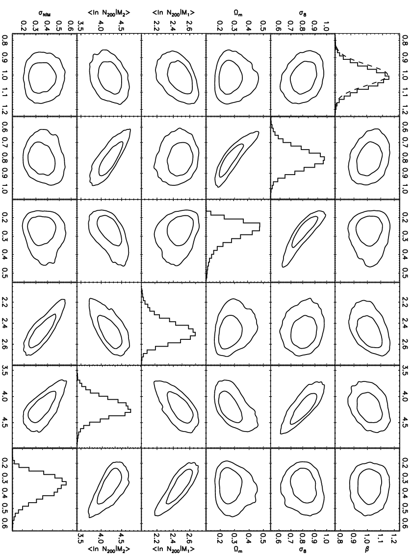
In the discussion that follows, we restrict ourselves to the subset of plots which we find most interesting. Throughout, unless otherwise noted we summarize constraints on a parameter by writing where and are the mean and standard deviation of the likelihood distribution for marginalized over all other parameters. We use this convention even when the likelihood function is obviously not Gaussian.
| Parametera | maxBCG | maxBCG+WMAP5b |
|---|---|---|
IV.1. Cosmological Constraints and Comparison to WMAP
The solid curves in Figure 5 show the and confidence regions from our analysis. The “thin” axis of our error ellipse corresponds to .44 4 The exponent is obtained by estimating the covariance matrix of and , and finding the best constrained eigenvector. The constraints on each of the individual parameters are and . The marginalized likelihood can be reasonably approximated by a log-normal distribution with , , and a correlation coefficient between and . Also shown in Figure 5 as dashed curves are the corresponding regions from the WMAP 5-year results (wmap08). Our results are consistent with WMAP5. Combining the two experiments results in the inner filled ellipses, given by and , with nearly no covariance between the two parameters (). These joint constraints on and represent nearly a factor of two improvement relative to the constraints from WMAP alone.
The shape of the confidence region is easy to interpret: since the number of massive clusters increases with both and , in order to hold the cluster abundance fixed at its observed value any increase in must be compensated by a decrease in , implying that a product of the form must be held fixed. The specific value of depends on the mass scale that is best constrained from the data. The particular degeneracy recovered by our analysis corresponds to a mass scale , which is about what we would expect (i.e. roughly half way between the lowest and highest masses probed by our data). Figure 6 illustrates this argument by showing the tinkeretal08 halo mass function weighted by the mass selection function from Figure 3 for two different cosmologies: a low (high ) cosmology, and a high (low ) cosmology, where the product has been held fixed to our best-fit value. We will refer back to Figure 6 multiple times in the following discussion.


IV.2. Constraints on the Richness–Mass Relation
In our analysis, we parameterized the richness–mass relation in terms of its scatter, and the value of the mean at two mass scales, and . We now re-parameterize this relation in terms of an amplitude and slope for , selecting as the pivot point the mass scale at which the uncertainty in is minimized. We write then
| (13) |
We find the error on the amplitude parameter is minimized for , which agrees well with the peak in the mass distribution of our clusters as shown in Figure 6. In what follows, we discuss only constraints on the richness–mass relation assuming this parameterization. A discussion of possible curvature in the richness–mass relation and/or mass scaling of its scatter is relegated to §V.3.
Figure 7 summarizes our constraints on the richness–mass relation after marginalizing over all other parameters. The best-fit values for each of the parameters are , , and . Note that for a pure power-law abundance function, one expects , in accordance with our result.
Of these results, the constraints on the slope and scatter of the richness–mass relation are particularly worth noting. First, it is clear that the naive scaling is not satisfied, with the slope of the richness–mass relation being significantly smaller than unity. Second, the recovered scatter is larger than the Poisson value that one might naively expect for clusters with galaxies, which is the typical richness of clusters at the mass scale where mass function is best constrained.
Interpreting these results in terms of standard halo occupation model parameters requires care. The maxBCG richness is known to suffer from various sources of systematics including miscentering of clusters (johnstonetal07b) and color off-sets in the richness estimates (rozoetal08b), both of which will impact the recovered richness–mass relation at some level. Moreover, any richness estimate will suffer to some extent from projection effects (cohnetal07), and discrepancies between assigned cluster radii and the standard mass-overdensity definitions used for halos. Disentangling the various contributions of each of these different sources of scatter to the total variance of the richness–mass relation is beyond the scope of this paper, and will not be considered further here.

Figure 7 also shows that the amplitude of the richness–mass relation is anti-correlated with the scatter. This is not surprising: at fixed cluster abundance, and given a fixed mass function, models with a high amplitude of the richness–mass relation result in halos that tend to be very rich. This means that the number of lower mass halos that scatter into higher richness must be low, or otherwise the abundance of clusters will be over-predicted. Consequently, high amplitude models must have low scatter, leading to an anti-correlation between the two parameters.
IV.3. Degeneracies Between Cosmology and the Richness–Mass Relation
Figure 4 shows that the most significant correlation between cosmology and our fiducial richness–mass relation parameters is that between and where is our higher reference mass . Because the pivot point for the mean of the richness–mass relation is so close to our original low mass reference scale used to define , it follows that must be closely related to , the slope of the richness–mass relation. We thus expect a strong degeneracy between and (rozoetal04, see also).
Figure 8 shows that this is indeed the case. We can understand the origin of this anti-correlation by investigating Figure 6. We have seen that the data fixes the amplitude of the halo abundance at . At the high mass end, however, the expected abundance of massive halos varies rapidly with . Low models result in fewer massive halos, so high richness clusters will have relatively lower masses. That is, richness must increase steeply with mass, and hence must be high, explaining the anti-correlation between and .
Figure 8 also demonstrates how these constraints are improved when we include a WMAP five-year data prior . This prior corresponds to the error along the thin direction of the WMAP error ellipse. Since WMAP data breaks the degeneracy in the data, including the WMAP prior produces a tight constraint in the plane. The new marginalized uncertainty in the slope of the richness–mass relation is , significantly smaller than unity.

V. Systematic Errors
We now consider the impact of three varieties of systematic errors on our analysis. Section V.1 investigates observational systematics, Section V.2 investigates systematics due to our assumed priors, and Section V.3 investigates systematics due to the parameterization of the richness–mass relation.
V.1. Observational Systematics
In this section, we study how observational systematics affect the recovered cosmological constraints from our analysis. We consider two such systematics: one, the impact of purity and completeness, and two, the impact of possible biases in the weak lensing mass estimates of the maxBCG clusters. We do not discuss uncertainties in the photometric redshifts for clusters at any length since, as discussed in Section III.4, they are found to be negligible. This is not surprising, as the maxBCG photometric redshift estimates are extremely accurate (koesteretal07a, ,).
V.1.1 The Impact of Purity and Completeness
Figure 9 compares the cosmological constraints obtained assuming perfect purity and completeness with those obtained assuming a uncertainty in these quantities. While non-negligible, the uncertainty in the completeness and purity function of the maxBCG catalog is far from the dominant source of uncertainty in our analysis. Moreover, this uncertainty elongates the error ellipse along its unconstrained direction, but has a minimal impact on the best constrained combination of and : in our fiducial analysis, while assuming perfect purity and completeness, a mere difference.
It is easy to understand why a uncertainty in the purity and completeness has a minimal impact in our results. For , the statistical uncertainties in the cluster abundances are larger than the uncertainty in the counts from purity and completeness. Since the best constrained combination of cosmological parameters is driven primarily by high mass clusters, a uncertainty in the purity and completeness functions has little impact on this parameter combination. How far the error ellipse extends along the degeneracy, however, is primarily driven by the observational constraints on the low end of the halo mass function (see Figure 6). Consequently, the systematic uncertainty in the low richness cluster counts elongates the error ellipse along its major axis.
We conclude that for the expected level of purity and completeness of the maxBCG cluster sample, our cosmological constraints are robust to these systematics.

V.1.2 Systematic Uncertainties of the Weak Lensing Mass Estimates
In Section II.2, we discussed that the weak lensing masses of johnstonetal07 were boosted by a factor of to account for biases arising from scatter in the photometric redshift estimates (mandelbaumetal08). Even with such a boost, the johnstonetal07 and the mandelbaumetal08b mass estimates were not consistent, which led us in Section III.2 to introduce a mass bias parameter that uniformly scales all masses by the same amount in order to account for any remaining biases. We now wish to explore how robust our results are to our estimate of this systematic uncertainty.
Figure 9 illustrates what happens if we repeat our fiducial analysis while doubling the width of the prior of from from to . We find that the wider prior significantly increases the uncertainty in the parameter combination from to , corresponding to a increase of the error bar. Using this new, wider prior, we find that the joint maxBCG + WMAP 5-year likelihood result in the cosmological constraints and , which constitute a increase in the uncertainty of each of these parameters respectively. Even with this wider prior, however, adding the maxBCG constraint to the WMAP5 result improves the final cosmological constraints on and by a factor of 1.6 relative to those obtained using WMAP data alone.
We can understand the impact of the mass bias parameter on our cosmological constraints using Figure 6. A wider prior on implies that the mass scale of the maxBCG clusters is more uncertain, so the mass at which the cluster abundance is best constrained, i.e. the point at which the two curves in Figure 6 cross each other, is more uncertain. Consequently, the cluster normalization constraint is weakened. The error along the long direction of the error ellipse does not change because the width of the mass range probed by the maxBCG clusters is largely independent of an overall mass bias.
One of the curious results that we have found in our study of the mass bias parameter is that the prior and posterior distributions of this parameter are different. In particular, we find that given the priors and , the posterior distributions for are and respectively. Indeed, this explains why the error ellipse for our wider prior is displaced to the left of that of our fiducial analysis: the shift in corresponds to a change in the mass scale, which has to be compensated by a change in the matter density parameter .
We conclude that the uncertainty in the weak lensing mass estimates of the maxBCG clusters is an important source of systematic uncertainty in our analysis. In fact, it is the dominant source of systematic uncertainty in our analysis. We have explicitly considered the impact of photometric redshift estimates for source galaxies as the source of this uncertainty, but other biases to the lensing masses — for example if the fraction of miscentered clusters was over- or under-estimated by johnstonetal07 — would affect our results in a similar way.
V.2. Prior-Driven Systematics
Our analysis makes use of two important priors: that the only two cosmological parameters of interest are and , and that the scatter in the richness–mass relation can be determined from X-ray studies as discussed in rozoetal08a. Here, we discuss how our results change if these priors are relaxed.
V.2.1 Cosmological Priors
After and , cluster abundance studies are most sensitive to the Hubble parameter and the tilt of the primordial power spectrum. In Figure 10, we illustrate how the constraints on the plane are affected upon marginalization over and using Gaussian priors and . As we can see, marginalizing over the Hubble parameter and the tilt of the power spectrum elongates the error ellipse, but it does not make it wider. Thus, the combination remains tightly constrained, and a joint maxBCG and WMAP 5-year data analysis is robust to the details of the priors used for and when estimating the maxBCG likelihood function. We also investigated whether a non-zero neutrino mass could significantly affect our results. Using a prior , we find that massive neutrinos do not significantly affect our constrain on . We conclude that holding the Hubble parameter and the tilt of the power spectrum fixed does not result in systematic uncertainties in the joint maxBCG + WMAP 5-year data analysis.

V.2.2 The Impact of the Scatter Prior
In rozoetal08a, we derived an empirical constraint on the scatter of the richness–mass relation by demanding consistency between X-ray, weak lensing, and cluster abundance data. The recovered scatter, however, characterized the richness–mass relation using a mass that was defined using an overdensity of 500 relative to the critical density of the universe. In this analysis, we use a density threshold of 200 relative to mean, so the use of the X-ray derived scatter prior is justified only if the scatter in the mass scaling between the two overdensity thresholds is not the dominant source of scatter. While we fully expect this assumption to hold, we have repeated our analysis without use of the scatter prior in order to cross-check our results.
Figure 10 summarizes our results. We find that our scatter prior tightens the error ellipse along both its short and long axis. This is as expected: without the scatter prior, the mass scale of the maxBCG clusters becomes less constrained, and consequently the halo mass function is less tightly constrained at all scales. The best constrained combination of and when dropping the rozoetal08a prior on the scatter in the mass–richness relation is . This value represents a increase in uncertainty relative to our fiducial analysis. The joint maxBCG + WMAP5 constraints in this case are and .
Not surprisingly, prior knowledge of the scatter of the mass–richness relation can significantly enhance the constraining power of the maxBCG data set. Nevertheless, even without prior knowledge in the scatter the joint maxBCG+WMAP constraints improve upon the WMAP values by a factor of 1.7.
V.3. Parameterization Systematics
One of the most important systematics that need to be addressed in studies where the observable–mass relation is parameterized in some simple way is how to assess the robustness of the results to changes in the parameterization of the observable–mass relation. Here, we have assumed that the richness–mass relation is a log-normal of constant scatter and that varies linearly with . We now investigate how our results change if we relax some of these assumptions.
V.3.1 Curvature in the Mean Richness–Mass Relation
To investigate the impact of curvature in the mass richness relation, we assume is a piecewise linear function. We first specify at three mass scales , , and , and define the value of at every other mass through linear interpolation in log-space. We set the minimum and maximum reference masses to the same values as before, , and . The intermediate reference mass is set to the geometric average of these two masses, , or . Note this mass scale is very nearly the same as the mass at which the halo mass function is best constrained.
Figure 11 shows how our cosmological constraints change with the introduction of mass dependence on the slope of the mean richness–mass relation . We find that the thin axis of the error ellipse is not significantly affected by this more flexible parameterization, while the long axis of the error ellipse is somewhat lengthened. This is as expected: the high mass end of the halo mass function is only sensitive to how richness varies with mass for large , and in this regime the more flexible parameterization does not introduce significantly more freedom. Thus, our data will tightly constrain the high mass end of the halo mass function just as well as did before, leading to no degradation in the error of . Once the high mass end of the richness–mass relation has been fixed, however, introducing curvature in dilutes the information contained in the low mass end of the halo mass function, thereby increasing the error ellipse along its long axis. Note the robustness of the constraint also implies that the constraints of a joint maxBCG + WMAP5 analysis are not significantly affected by our choice of parameterization.

Irrespective of the impact our new parameterization of has on our cosmological constraints, it is fair to ask whether or not there is significant evidence for curvature of the mean richness–mass relation. Using a maximum likelihood ratio test, we find that the increase in likelihood due to curvature in the richness–mass relation is significant at the level, less than . Thus, there is no evidence for curvature in the richness–mass relation. We have also explicitly confirmed that the slopes of the low and high mass end of the richness–mass relation are consistent with each other. Indeed, we find
| (14) |
where we have assumed
| (15) |
and .
V.3.2 Scaling of the Scatter in the Richness–Mass Relation with Mass
We now investigate whether allowing the scatter of the richness–mass relation to vary with mass has a significant impact on our cosmological parameters. For these purposes, we allow the scatter to vary linearly with , and parameterize it by specifying its values at the reference masses and . The value of at any other mass is obtained through linear interpolation.
Figure 11 compares the cosmological constraints we obtain with our new model to those of our fiducial analysis with constant scatter. Once again, we find that the “thin” axis of the error ellipse is not significantly affected by the new more flexible parameterization, while the long axis is slightly elongated. The interpretation of these results is the same as those of §V.3.1. We have tested for evidence of scaling of the scatter in the richness–mass relation with halo mass using a likelihood ratio test. The increase in likelihood due to a linearly varying scatter is significant at the level, implying there is no evidence of mass dependence in the scatter of the richness–mass relation in the data. We have also explicitly confirmed that the scatter at the low and high mass ends probed by the maxBCG cluster sample are consistent with each other. Indeed, our constraint on the slope of the mass dependence of the scatter in the richness–mass relation is
| (16) |
where we assumed
| (17) |
We note the velocity dispersion analysis in beckeretal07 points towards some mass dependence in the scatter of the mass–richness relation, though part of this discrepancy is likely due to miscentering systematics (see rozoetal08a, for details). We are now in the process of reanalyzing the velocity dispersion data updating both our treatment of systematics, and substantially increasing the sample of spectroscopically sampled galaxies, so we defer a detailed discussion of these results to a future paper.
We conclude that our parameterization of the mean and scatter of the richness–mass relation does not introduce systematic errors in our analysis.
V.3.3 Richness Range Considered
We have tested whether there is cosmological information in the richness range by running MCMCs both with and without the contribution of these clusters to the likelihood function. We find that these two analyses yield nearly identical results. We have also explicitly confirmed that our results are robust to the lowest richness bin employed in the analysis. As we might expect, removing the lowest richness bin increases our uncertainties along the long axis of the error ellipse as shown in Figure 12. We also investigate adding a new lowest richness bin, consisting of clusters in with 9–10, as well as the mean mass for clusters in the range 9–11. This analysis rotates the error ellipse very slightly compared to our fiducial analysis, but does not significantly affect our results.

VI. Discussion
VI.1. Comparison to Other Work
The main point of this section is to demonstrate two points:
- 1.
The cosmological constraints from the maxBCG cluster catalog are competitive with the state of the art constraints derived from low redshift X-ray selected cluster samples.
- 2.
Despite the markedly different analyses and sources of systematic uncertainty, the cluster abundance constraints from the maxBCG cluster sample are in excellent agreement with those of X-ray selected samples. This demonstrates the robustness of cluster abundance studies as a tool of precision cosmology.
Given our goal, in this section we focus exclusively on the most recent cosmological constraints derived from low redshift X-ray cluster samples. In particular, we explicitly consider only three works: mantzetal08, who worked with the X-ray luminosity function, henryetal08, who worked with the X-ray temperature function, and vikhlininetal08b, who estimated the low redshift halo mass function using the 400d X-ray survey (bureninetal07) with mass estimates based on (kravtsovetal06). These three papers are the most recent analyses of X-ray selected cluster samples, and all recover tight cosmological constraints that are in excellent agreement with one another, while carefully accounting for the relevant systematics for each of their analyses.
Now, as we have discussed in previous sections, the main result from low redshift cluster abundance studies is a tight constraint on the value of where for maxBCG clusters . Other cluster samples, however, will have slightly different values of , which brings up the question of how can we fairly compare these various constraints. One way would be to simply quote the percent uncertainty in the relevant combination. However, we would like to have a clear graphical representation of this result. We have chosen to do this by plotting the confidence regions of a simplified version of a joint cluster abundance + WMAP5 analysis assuming a neutrino-less flat CDM cosmology. We proceed as follows: given a cluster abundance experiment, we consider only the constraint on , disregarding all other cosmological information. We then add a WMAP 5 prior , which corresponds to the thin axis of the error WMAP5 error ellipse in the plane, and we compute the corresponding confidence regions in the plane.
