The topology of the space of matrices of Barvinok rank two

Let $P=\{p_{1},\dots,p_{d}\}$ and $Q=\{q_{1},\dots,q_{n}\}$ be disjoint sets of cardinality $d$ and $n$, respectively.

We now describe an abstract simplicial complex with $B_{d,n}$ as geometric realization. The simplices are encoded by combinatorial trees whose leaves are marked using $P$ and $Q$ as label sets. This model is equivalent to that given by Develin in [4, §  3].²² 2 To translate from our trees to those of [4], simply replace the leaf labelled $p_{i}$ and its incident edge by a leaf “heading off to infinity in the $i$-th coordinate direction”, and replace the leaf labelled $q_{i}$ and its incident edge by the $i$-th marked point. A completely analogous description in the context of matrices of tropical rank $2$ was given by Markwig and Yu [12]; their complex is denoted $\mathcal{T}_{d,n}$ below.

Consider the set of trees $\mathcal{T}$ with leaf set $P\cup Q$ such that every internal vertex (i.e. non-leaf) has degree at least three. We may think of $\mathcal{T}$ as a simplicial complex in the following way. The vertex set of the complex consists of all bipartitions of $P\cup Q$, and we identify a tree $\tau\in\mathcal{T}$ with the simplex comprised of the bipartitions induced by the connected components that arise when an internal edge (one not incident to a leaf) of $\tau$ is removed. (It is well-known, and easy to see, that there is at most one tree giving rise to any given set of bipartitions.) Clearly, the simplices in the boundary of $\tau$ are those obtained by contracting internal edges.

Let $\mathcal{T}_{d,n}$ be the subcomplex of $\mathcal{T}$ which is induced by the bipartitions where both parts have nonempty intersection with both $P$ and $Q$. Our main object of study is the subcomplex of $\mathcal{T}_{d,n}$ which consists of the trees whose internal vertices form a path as induced subgraph. Let us denote this complex by $\mathcal{B}_{d,n}$.

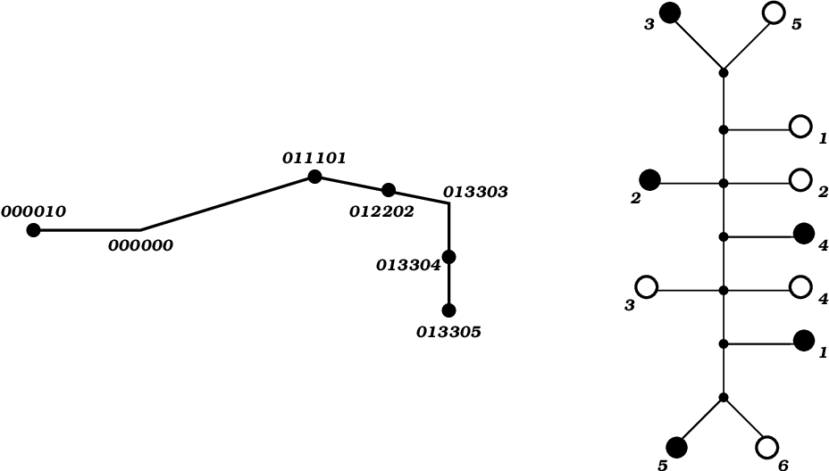
Specifically, a matrix $M\in B_{d,n}$ is associated with a tree in $\mathcal{B}_{d,n}$ as follows. Let $c_{1},\dots,c_{n}$ denote the columns of $M$. Then, $T=\mathrm{tconv}(c_{1},\dots,c_{n})$ is a tropical line segment in $\mathbb{TP}^{d-1}$. Now construct a tree $\tau=\tau(M)$ whose internal vertex set is the union of $\{c_{1},\dots,c_{n}\}$ and the set of points where the curve $T$ is not smooth. Two internal vertices $v_{1}\neq v_{2}$ are adjacent if and only if $\mathrm{tconv}(v_{1},v_{2})$ (which is a subset of $T$) contains no other internal vertex. The leaf set of $\tau$ is $P\cup Q$. The leaf $p_{i}$ is adjacent to the internal vertex which is closest to the origin (which, by Condition (ii) of Definition 3.1, is necessarily an internal vertex) among those where the $i$-th coordinate is maximized. Finally, the leaf $q_{i}$ is adjacent to the vertex $c_{i}$. The resulting tree (seen as an abstract, leaf-labelled tree) is $\tau$.

Our next goal is to prove that $\mathcal{B}_{d,n}$ is homeomorphic to $(S^{d-2}\times S^{n-2})/\mathbb{Z}_{2}$, where the generator of $\mathbb{Z}_{2}$ acts by the antipodal map on both components.

For a set $S$, let $\mathfrak{b}(S)$ denote the proper part of the Boolean lattice on $S$. Thus, $\mathfrak{b}(S)$ is the poset of all proper, nonempty subsets of $S$ ordered by inclusion.

Recall our sets $P$ and $Q$. The chains in $\mathfrak{b}(P)\times\mathfrak{b}(Q)$ can be thought of as compositions (i.e. ordered set partitions) of $P\cup Q$ such that the first and the last block both have nonempty intersection with both $P$ and $Q$; let us for brevity call such compositions balanced. Namely, a chain $(S_{1},T_{1})<\cdots<(S_{k},T_{k})$ corresponds to the balanced composition $(C_{1},\dots,C_{k+1})$, where

identifying $S_{k+1}$ and $T_{k+1}$ with $P$ and $Q$, respectively. Under this bijection, inclusion among chains corresponds to refinement among compositions.

Let $\Delta(\cdot)$ denote order complex³³ 3 The order complex of a finite poset is the abstract simplicial complex whose simplices are the totally ordered subsets.. We have a map of simplicial complexes $\varphi:\Delta\left(\mathfrak{b}(P)\times\mathfrak{b}(Q)\right)\to\mathcal{B}_{d,n}$ by sending a balanced composition $C=(C_{1},\dots,C_{k})$ to the unique tree $\varphi(C)\in\mathcal{B}_{d,n}$ in which $C_{i}$ is the set of leaves adjacent to the $i$th internal vertex, counting along the internal path from one of the endpoints. As an example, there are two balanced compositions that are mapped to the tree in Figure 2, namely $(p_{5}q_{3},p_{1},p_{2}q_{2},q_{4},p_{3}p_{4},q_{1},p_{6}q_{5})$ and its reverse composition $(p_{6}q_{5},q_{1},p_{3}p_{4},q_{4},p_{2}q_{2},p_{1},p_{5}q_{3})$.

Conversely, for $\tau\in\mathcal{B}_{d,n}$, suppose the path from one endpoint of the internal path to the other traverses the internal vertices in the order $v_{1},\dots,v_{k}$. Let $C_{i}\subset P\cup Q$ be the set of leaves adjacent to $v_{i}$. Clearly,

This shows that $\varphi$ induces an isomorphism of simplicial complexes:

where the generator of $\mathbb{Z}_{2}$ acts by taking complement inside $\mathfrak{b}(P)$ and $\mathfrak{b}(Q)$ simultaneously.

Given finite posets $\Pi$ and $\Sigma$, the product space $\Delta(\Pi)\times\Delta(\Sigma)$ has a natural cell complex structure, where the cells are of the form $\Delta(C^{\Pi})\times\Delta(C^{\Sigma})$ for chains $C^{\Pi}\subseteq\Pi$, $C^{\Sigma}\subseteq\Sigma$. It is well known [7, Lemma 8.9] that $\Delta(\Pi\times\Sigma)$ is a simplicial subdivision of $\Delta(\Pi)\times\Delta(\Sigma)$, a cell $\Delta(C^{\Pi})\times\Delta(C^{\Sigma})$ being subdivided by $\Delta(C^{\Pi}\times C^{\Sigma})$.

In particular, $\Delta\left(\mathfrak{b}(P)\times\mathfrak{b}(Q)\right)\cong\Delta\left(\mathfrak{b}(P)\right)\times\Delta\left(\mathfrak{b}(Q)\right)$. Moreover, the $\mathbb{Z}_{2}$-action clearly respects the subdivision so that we obtain

where the generator of $\mathbb{Z}_{2}$ acts by taking complementary chains in both $\mathfrak{b}(P)$ and $\mathfrak{b}(Q)$.

Finally, it is well known that $\Delta\left(\mathfrak{b}(S)\right)$ is homeomorphic to the $(|S|-2)$-sphere, and that the complement map on $\mathfrak{b}(S)$ corresponds to the antipodal map on the sphere. This concludes the proof of Theorem 1.1.

Let us consider the special case of interest in our calculation of the homology of $B_{d,n}$. Write $D=d-2$ and $N=n-2$. For $0\leq i\leq D$, let $V_{i}$ be a free $R$-module generated by two elements $\sigma_{i}^{+}=\sigma_{i}^{+1}$ and $\sigma_{i}^{-}=\sigma_{i}^{-1}$; set $V_{i}=0$ for $i<0$ and $i>D$. We define

for $\epsilon=\pm 1$. This means that $\mathsf{V}$ is the unreduced chain complex corresponding to the standard hemispherical cell decomposition of the $D$-sphere. A $\mathbb{Z}_{2}$-action is given by mapping $\sigma_{i}^{+}$ to $\sigma_{i}^{-}$ and vice versa. This corresponds to the antipodal action on the sphere, and $\mathsf{V}^{+}$ consequently corresponds to the minimal cell decomposition of real projective $D$-space [9, Ex. 2.42]. We refer to $\mathsf{V}$ as the standard hemispherical chain complex over $R$ of degree $D$. Using Theorem 1.1, we deduce the following.

First we consider the case that $2$ is a unit in $R$.

Let $\mathsf{C}$ be a chain complex of $R$-modules with an involution $\iota$. Then, we may write each element $c$ uniquely as a sum $c=a+b$ such that $a=\iota(a)$ and $b=-\iota(b)$. Namely, $a=\frac{1}{2}(c+\iota(c))$ and $b=\frac{1}{2}(c-\iota(c))$. This means that $\mathsf{C}^{+}$ can be identified with the subcomplex of elements $a$ satisfying $a-\iota(a)=0$ and $\mathsf{C}^{-}$ with the subcomplex of elements $b$ satisfying $b+\iota(b)=0$. Moreover, we may identify $\mathsf{C}$ with the direct sum $\mathsf{C}^{+}\oplus\mathsf{C}^{-}$.

Applying the above to each of $\mathsf{V}$ and $\mathsf{W}$, we obtain that

We have that $\iota(x)=x$ if

and $\iota(x)=-x$ if

As a consequence,

Applying Künneth’s theorem [9, Th. 3B.5], we obtain the following result.

Suppose that $\mathsf{V}$ is the standard hemispherical chain complex of degree $D$. By Lemma 4.2, we have that $H_{i}(\mathsf{V}^{+})\cong H_{i}(\mathsf{V}^{-})\cong 0$ unless $i=0$ or $i=D$. Moreover, $H_{0}(\mathsf{V}^{+})\cong R$ and $H_{0}(\mathsf{V}^{-})\cong 0$. Finally, if $D$ is odd, then $H_{D}(\mathsf{V}^{+})\cong R$ and $H_{D}(\mathsf{V}^{-})\cong 0$. If instead $D$ is even, then $H_{D}(\mathsf{V}^{+})\cong 0$ and $H_{D}(\mathsf{V}^{-})\cong R$. The following assertion is an immediate consequence:

Identifying $\mathsf{V}$ and $\mathsf{W}$ with the cellular chain complexes corresponding to the hemispherical cell decompositions of the $(d-2)$-sphere and the $(n-2)$-sphere, respectively, yields the following corollary, which could also be deduced using transfer methods; see e.g. Bredon [2, §  III].

To compute the homology of $\left({\sf V}\otimes{\sf W}\right)^{+}$ in the case that $2$ is not a unit in $R$, we will use an algebraic version [10, § 4.4] of discrete Morse theory [8].

The general situation is that we have a chain complex ${\sf C}$ of finitely generated $R$-modules $C_{i}$. Write $C=\bigoplus_{i}C_{i}$. Assume that $C$ can be written as a direct sum of three $R$-modules $A$, $B$, and $U$ such that $f=\alpha\circ\partial$ defines an isomorphism $f:B\rightarrow A$, where $\alpha(a+b+u)=a$ for $a\in A,b\in B,u\in U$. Let $h:A\rightarrow B$ be the inverse of $f|_{B}$. For any chain group element $x$, define $\beta(x)=h\circ f(x)$ and $\hat{U}=(\text{id}-\beta)(U)$. Let $\hat{U}_{k}$ be the component of $\hat{U}$ in degree $k$.

For the connection to discrete Morse theory [8], consider a matching on the set of cells in a cell complex such that each pair in the matching is of the form $(\sigma,\tau)$, where $\sigma$ is a regular codimension one face of $\tau$. Let $A$ be the free $R$-module generated by cells matched with larger cells, let $B$ be generated by cells matched with smaller cells, and let $U$ be generated by unmatched cells. Then, the map $f:B\rightarrow A$ is an isomorphism if the matching is a Morse matching [3], and $\hat{\sf U}$ is the Morse complex associated to the matching.

In the case that $2$ is not a unit, the discussion in Section 4.2 does not apply, as the chain complex no longer splits in the manner described. In fact, the situation is considerably more complicated. For this reason, we only examine the special case that ${\sf V}$ is the standard hemispherical chain complex of degree $D$.

We also need some assumptions on $\mathsf{W}$. Specifically, we assume that we may write $W_{j}$ as a direct product $L_{j}\times L_{j}$, where $L_{j}$ is a finitely generated $R$-module for each $j\in\mathbb{Z}$. Moreover, we assume that $\iota(w_{0},w_{1})=(w_{1},w_{0})$ for each element $(w_{0},w_{1})\in W_{j}$. For our main result to hold, we must assume that $L_{j}=0$ unless $0\leq j\leq D$. However, we will not actually use this assumption until Lemma 4.10.

We make no specific assumptions on the boundary operator on $\mathsf{W}$, which hence is of the general form

where $p,q,r,s$ are maps $L_{j}\rightarrow L_{j-1}$ such that $\partial^{2}=0$ and $\iota\partial=\partial\iota$. Since $\iota(w,0)=(0,w)$, we have that

and hence that

For $\partial^{2}$ to be zero, it is necessary and sufficient that $p^{2}+q^{2}=pq+qp=0$.

Recall that we want to examine $(\mathsf{V}\otimes\mathsf{W})^{+}$. In this chain complex, we have for each $i$ and $w_{0},w_{1}\in L_{j}$ the identity

In particular, we may identify $(V_{i}\otimes W_{j})^{+}$ with $\langle\sigma_{i}^{+}\rangle\otimes W_{j}\cong W_{j}\mathbf{e}_{i,j}$, where $\mathbf{e}_{i,j}$ is a formal variable. Writing $\epsilon=-1$ for compactness, also note that

Identifying $(V_{i}\otimes W_{j})^{+}$ with $W_{j}\mathbf{e}_{i,j}$ as described above, we may express this as

We want to use Proposition 4.6 to simplify $(\mathsf{V}\otimes\mathsf{W})^{+}$. For $0\leq i\leq D$ and $j\in\mathbb{Z}$, define

Note that $(V_{i}\otimes W_{j})^{+}\cong(L_{j}\times L_{j})\mathbf{e}_{i,j}$ is isomorphic to the direct sum of $L_{j}{\bf a}_{i,j}$ and $L_{j}{\bf b}_{i,j}$. Define

See Table 1 for a schematic description. Write $U=U^{(0)}\oplus U^{(D)}$. Note that the direct sum of $A$, $B$, and $U$ constitutes the full chain complex $\left({\sf V}\otimes{\sf W}\right)^{+}$.

It is clear that we obtain an isomorphism $g:B\rightarrow A$ by assigning $g(w{\bf b}_{i,j})=w{\bf a}_{i-1,j}$ for each $i$ and $j$ and each $w\in L_{j}$. We now show that discrete Morse theory indeed yields an isomorphism between $B$ and $A$, though the assignment is slightly more complicated. Let $\alpha$ be the projection map from $A+B+U$ to $A$ as defined in Section 4.3, and let $f=\alpha\circ\partial$.

References

- [1] A. Barvinok, S. P. Fekete, D. S. Johnson, A. Tamir, G. J. Woeginger, and R. Woodroofe, The geometric maximum traveling salesman problem, J. ACM 50 (2003), 641–664.
- [2] G. E. Bredon, Introduction to compact transformation groups, Academic Press, New York, 1972.
- [3] M. K. Chari, On discrete Morse functions and combinatorial decompositions, Discrete Math. 217 (2000), No. 1-3, 101–113.
- [4] M. Develin, The moduli space of tropically collinear points in , Collect. Math. 56 (2005), 1–19.
- [5] M. Develin, F. Santos, and B. Sturmfels, On the rank of a tropical matrix, J. E. Goodman, J. Pach and E. Welzl, Editors, Discrete and Computational Geometry vol. 52, MSRI Publications, Cambridge University Press, 2005, 213–242.
- [6] M. Develin, B. Sturmfels, Tropical convexity, Doc. Math. 9 (2004), 1–27.
- [7] S. Eilenberg and N. Steenrod, Foundations of Algebraic Topology, Princeton University Press, 1952.
- [8] R. Forman, Morse theory for cell complexes, Adv. in Math. 134 (1998), 90–145.
- [9] A. Hatcher, Algebraic Topology, Cambridge University Press, 2002.
- [10] J. Jonsson, Simplicial Complexes of Graphs, Lecture Notes in Mathematics 1928, Springer, 2008.
- [11] G. L. Litvinov, The Maslov dequantization, idempotent and tropical mathematics: a very brief introduction, In Idempotent mathematics and mathematical physics, Contemp. Math. 377, Amer. Math. Soc., Providence, RI, 2005, 1–17.
- [12] H. Markwig, J. Yu, The space of tropically collinear points is shellable, Collect. Math. 60 (2009), 63–77.
- [13] G. Mikhalkin, Tropical geometry and its applications, Proceedings of the International Congress of Mathematicians, Madrid 2006, 827–852.