Orientation in Social Networks

In a network, if there exist a path form node $p_{m}$ to node $p_{0}$: $p_{m}\rightarrow p_{m-1}\rightarrow\cdots\rightarrow p_{0}$, then there must be a corresponding intimacy spreading path $p_{0}\rightarrow p_{1}\rightarrow\cdots\rightarrow p_{m}$ which we call intimacy spreading path form $p_{0}$ to $p_{m}$. That’s to say we send message alone $p_{m}\rightarrow p_{m-1}\rightarrow\cdots\rightarrow p_{0}$, and get nodes information alone $p_{0}\rightarrow p_{1}\rightarrow\cdots\rightarrow p_{m}$. It is obvious that there exist a intimacy spreading path from $p_{0}$ to $p_{m}$, there must be a path from $p_{m}$ to $p_{0}$.

Theorem 1: Suppose $a>>1$ and there exist a constant $H$ such that for any positive $m$, $\prod_{i=1}^{m}(k_{i}a+k_{i}-1)\approx H^{m}$ in statistic sense, where $k_{i}$ is the out degree of node $i$ (it is strict in lattice based networks). Then intimacy degree of $p_{m}$ possessed about $p_{0}$ will decay with the length of their shortest path exponentially, and will decay inversely to the degree of the node by which intimacy passes.

Proof:

Suppose $p_{i}$ has $k_{i}$ neighbors, $N_{p_{1}}^{1},N_{p_{1}}^{2},\cdots,N_{p_{1}}^{k_{1}}$ denote all the neighbors of $p_{1}$ and $p_{0}$ is a neighbor of $p_{1}$, $v^{T}_{x}(y)$ denotes the intimacy degree of node $x$ to node $y$ after $T$ steps evolution, $v^{0}_{x}(y)=a$ if $y$=$x$, otherwise $0$. Without losing generality we let $p_{0}=N_{p_{1}}^{1}$.

$\because\$ $p_{0}\rightarrow p_{1}\rightarrow\cdots\rightarrow p_{m}$ is an intimacy spreading path from $p_{0}$ to $p_{m}$.

$\therefore\$ from the Eq.1 we have $v^{T}_{p_{1}}(p_{0})=\frac{\sum_{i=1}^{k_{1}}v^{T-1}_{N_{p_{1}}^{i}}(p_{0})}{\sum_{i=1}^{k_{1}}\sum_{j=1}^{n}v^{T-1}_{N_{p_{1}}^{i}}(j)-\sum_{i=1}^{k_{1}}v^{T-1}_{N_{p_{1}}^{i}}(p_{1})}=\frac{a+\sum_{i=2}^{k_{1}}v^{T-1}_{N_{p_{1}}^{i}}(p_{0})}{k_{1}a+k_{1}-\sum_{i=1}^{k_{1}}v^{T-1}_{N_{p_{1}}^{i}}(p_{1})}$

$\because\ 0<v^{T-1}_{N_{p_{1}}^{i}}(p_{0})\leq 1,i=1,\cdots,k_{1}$

$\therefore\ \frac{a}{k_{1}a+k_{1}}\leq v^{T-1}_{p_{1}}(p_{0})\leq\frac{a+k_{1}}{k_{1}a}$

$\because\ a\gg 1$

$\therefore\ v^{T}_{p_{1}}(p_{0})\thickapprox\frac{1}{k_{1}}$, $T=1,2\cdots+\infty$

$\therefore\ v^{T}_{N_{p_{i}}^{j}}(p_{i})\thickapprox\frac{1}{k_{i}}$, $T=1,2\cdots+\infty$

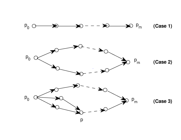
Case 1 (see Fig. 4 case 1): suppose there exist only one shortest path ($p_{m}\rightarrow p_{m-1}\rightarrow\cdots\rightarrow p_{0}$) from $p_{m}$ to $p_{0}$, then when the intimacy of $p_{0}$ spread to $p_{i}$ currently alone $p_{0}\rightarrow p_{1}\rightarrow\cdots\rightarrow p_{m}$.

Then the first intimacy degree (It means the intimacy degree possessed in the first time of one pair of nodes)    $v_{p_{i}}(p_{0})=\frac{v_{p_{i-1}}(p_{0})}{k_{i}a+k_{i}-\sum_{h=1}^{k_{i}}v_{N_{p_{i}}^{h}}(p_{i})}$ $\approx\,\frac{v_{p_{i-1}}(p_{0})}{k_{i}a+k_{i}-k_{i}\frac{1}{k_{i}}}=\frac{v_{p_{i-1}}(p_{0})}{k_{i}a+k_{i}-1}$ where, $N_{p_{i}}^{1},\cdots,N_{p_{i}}^{k_{i}}$ are $k_{i}$ neighbors of $p_{i}$ and $N_{p_{i}}^{1}=p_{i-1}$. (The above equation also implies the intimacy degree will decay inversely ($\frac{1}{k_{i}a}$) to the degree of the node by which intimacy passes.)

In this way we have:   $v_{p_{m}}(p_{0})=a\prod_{i=1}^{m}\frac{1}{k_{i}a+k_{i}-1}$

$\because\,\,\,\prod_{i=1}^{m}(k_{i}a+k_{i}-1)\approx H^{m}$

Then we have    $v_{p_{m}}(p_{0})\approx aH^{-m}$

Case 2 (see Fig. 4 case 2): When there are $r$ independent (means there is no common node for each pair of shortest pathes) shortest intimacy spreading pathes from $p_{0}$ to $p_{m}$ through $r$ neighbors of $p_{m}$. Assume the length of the shortest intimacy spreading pathes from $p_{0}$ to $p_{m}$ is $m$,then we can easily get that

$v_{p_{m}}(p_{0})\approx\frac{raH^{-(m-1)}}{ak_{m}+k_{m}-1}\,\approx\,raH^{-m}$

Case 3 (see Fig. 4 case 3): When there are $r$ shortest intimacy spreading pathes from $p_{0}$ to $p_{m}$ in which $\beta$ shortest intimacy spreading pathes are dependent and other $r-\beta$ are independent. All the situations are equal to this situation: all of the $\beta$ dependent intimacy spreading pathes encounter at node $p$ and they are independent from $p_{0}$ to $p$ and there only one shortest intimacy spreading path for $p$ to $p_{m}$. Assume the length of shortest intimacy spreading pathes from $p_{0}$ to $p_{m}$ is $m$, from $p_{0}$ to $p$ is $m_{1}$ and $p$ to $p_{m}$ is $m_{2}=m-m_{1}$.

According to case $1$ and case $2$ we have

$v_{p_{m}}(p_{0})\approx(r-\beta)aH^{-m}+(taH^{-m_{1}})H^{-m_{2}}\,=\,raH^{-m}$

Now, the task we face is to prove $v^{T}_{p_{m}}(p_{0})\approx raH^{-m}$ for any $T>=m$.

Obviously, $v^{T}_{p_{m}}(p_{0})$ equal the sum of the each step ($m$ to $T$) first intimacy degree, then we have :

$\,raH^{-m}=v_{p_{m}}(p_{0})\leq v^{T}_{p_{m}}(p_{0})\leq\,raH^{-m}+a[\frac{K^{m+1}}{a^{m+1}}+\frac{K^{m+2}}{a^{m+2}}+,\cdots,+\frac{K^{T}}{a^{T}}]$ where $K$ is the maximum out degree of all nodes.

Thus, $v^{T}_{p_{m}}(p_{0})\leq raH^{-m}+a[\frac{K^{m+1}}{a^{m+1}}+\int_{m+1}^{+\infty}(\frac{K}{a})^{x}dx]\leq raH^{-m}+2a\frac{K^{m+1}}{a^{m+1}}$

$\because\,\,\,\lim_{a\rightarrow\infty}\frac{2\frac{K^{m+1}}{a^{m+1}}}{H^{-m}}=0$

$\therefore\,\,\,$ for sufficient large $a$, $v^{T}_{p_{m}}(p_{0})\approx raH^{-m}$.

Theorem 2: For a connected network and $a>1$. If $i$ is not the target $t$ then there must be at least one neighbor $q$ of node $i$, $q$ is more intimate with target $t$ compared to node $i$ after sufficient long time evolution. This means that the message will not pass a node twice in the one sending process and always can reach the target $t$.

Proof:

$\because$ the network is connected

$\therefore$ node $i$ at lest has a neighbor.

Assume $i$ has $k_{i}$ neighbors which are $N_{i}^{1},N_{i}^{2},\cdots,N_{i}^{k_{i}}$.

$\because\ v^{+\infty}_{i}(j)=\frac{v^{+\infty}_{N_{i}^{1}}(j)+v^{+\infty}_{N_{i}^{2}}(j)+\cdots+v^{+\infty}_{N_{i}^{k_{i}}}(j)}{k_{i}a+k_{i}-\sum_{d=1}^{k_{i}}v^{+\infty}_{N_{i}^{d}}(i)}$ and $k_{i}a+k_{i}-\sum_{d=1}^{k_{i}}v^{+\infty}_{N_{i}^{d}}(i)>k_{i}$

$\therefore\,\,\,v^{+\infty}_{i}(j)<\max\{v^{+\infty}_{N_{i}^{1}}(j),v^{+\infty}_{N_{i}^{2}}(j),\cdots,v^{+\infty}_{N_{i}^{k_{i}}}(j)\}$

Therefore the above $q$ must be existed and in the a sending process, the current message holder will always more intimacy with target $t$ than the all previous message holder which implies that the message will not pass a node twice. Because the number of node of a network is finite, the message will and can reach the target $t$.

References

- [1] Milgram, S. Psych. Today 2, 60 (May 1967).
- [2] Karinthy, F., Chains. Everything is different. Budapest, (1929).
- [3] Guare, J. Six degrees of separation: a play. Vintage, New York, (1990).
- [4] Dodds, P. S., Muhamad,R., Watts, D. J. An Experimental Study of Search in Global Social Networks Science 301, 827 (2003)
- [5] Fiona Macrae, Microsoft proves you ARE just six degrees of separation from anyone in the world, Mailonline, Science and Tech, 04th August 2008, http://www.dailymail.co.uk/sciencetech/article-1041077/Microsoft-proves-ARE-just-degrees-separation-world.html.
- [6] Watts, D., Strogatz, S. Collective dynamics of small world Networks. Nature 393, 440-442 (1998).
- [7] S. H. Strogatz, Nature 410, 268 (2001).
- [8] Albert, R. and Barabsi, A.-L. Statistical mechanics of complex networks. Reviews of Modern Physics, 74, (2002).
- [9] Newman, M. E. J. The structure and function of complex networks. SIAM Review, 45, 167¨C256, (2003).
- [10] Kleinberg, J. M. Navigation in a small world. Nature 406, 845 (2000).
- [11] Kleinberg, J. M. The Small-World Phenomenon: An Algorithmic Perspective. In Proceedings of the 32nd ACM Symposium on Theory of Computing, (2000).
- [12] Kleinberg, J. M. Small-World Phenomena and the Dynamics of Inforamtion. In Advances in Neural Information Processing Systems (NIPS) 14, (2001).
- [13] Watts, D. J., Dodds,P. S. and Newman, M. E. J. Identity and search in social networks. Science, 296, 1302-1305, (2002).
- [14] Adamic, L., Lukose, R. A., Puniyani, A. R. and Huberman, B. A. Search in power-law networks. Physical Review E, 64, 46135, (2001).
- [15] Liben-Nowell, D., Novak, J., Kumar, R., Raghavan, P. and Tomkins, A. Geograph routing in social networks. In Proceedings of the National Academy of Science, 102, 11623-11628, (2005).
- [16] Fraigniaud, P., Gavoille, C., Kosowski, A., Lebhar, E. and Lotker, Z. in Proc. Nineteenth Annual ACM Symp. on Parallel Algorithms and Architectures. 1-7, ACM, (2007).
- [17] Fraigniaud, P. and Gavoille, C. in Proc. Twentieth Annual Symposium on Parallelism in Algorithms and Architectures. 62-69, ACM, (2008) SPAA. 29.
- [18] Sandberg, O. Searching in a Small World, University of Gothenburg and Chalmers Technical University (licentiate thesis), (2005).
- [19] Martel, C. and Nguyen, V. Analyzing kleinberg¡¯s (and other) small-world models. In PODC ¡¯04: Proceedings of the twentythird annual ACM symposium on Principles of distributed computing, pages 179¨C188, New York, NY, USA, ACM Press. (2004).
- [20] Barriere, L., Fraigniaud, P., Kranakis, E., Krizanc, D. Efficient Routing in Networks with Long Range Contacts, Proc. 15th Intr. Symp. on Dist. Computing, DISC 01, 270-284, (2001).
- [21] Adamic, L. and Adar, E. How to search a social network. Social Networks, 27, 187-203, (2005).
- [22] Bogu, M., Krioukov, D. and Claffy, K. C. Navigability of complex networks. Nature Physics, advance online publication, NPHYS1130, (2008).
4 Supplementary
4.1 Theorems and proof
In a network, if there exist a path form node to node : , then there must be a corresponding intimacy spreading path which we call intimacy spreading path form to . That’s to say we send message alone , and get nodes information alone . It is obvious that there exist a intimacy spreading path from to , there must be a path from to .
Theorem 1: Suppose and there exist a constant such that for any positive , in statistic sense, where is the out degree of node (it is strict in lattice based networks). Then intimacy degree of possessed about will decay with the length of their shortest path exponentially, and will decay inversely to the degree of the node by which intimacy passes.
Proof:
Suppose has neighbors, denote all the neighbors of and is a neighbor of , denotes the intimacy degree of node to node after steps evolution, if =, otherwise . Without losing generality we let .
is an intimacy spreading path from to .
from the Eq.1 we have