Branching Ratios, Forward-backward Asymmetry and Angular Distributions of $B\to K_{1}l^{+}l^{-}$ Decays

Run-Hui Li^a,b, Cai-Dian Lü^a,c and Wei Wang^a Note: wwang@mail.ihep.ac.cn Affiliation: ^a Institute of High Energy Physics, P.O. Box 918(4) Beijing 100049, People’s Republic of China
^b School of Physics, Shandong University, Jinan 250100, People’s Republic of China
^c Theoretical Physics Center for Science Facilities, Beijing 100049, People’s Republic of China

Abstract

Using the $B\to K_{1}$ form factors evaluated in the perturbative QCD approach, we study semileptonic $B\to K_{1}(1270)l^{+}l^{-}$ and $B\to K_{1}(1400)l^{+}l^{-}$ decays, where $K_{1}(1270)$ and $K_{1}(1400)$ are mixtures of $K_{1A}$ and $K_{1B}$ which are ${}^{3}P_{1}$ and ${}^{1}P_{1}$ states, respectively. Using the technique of helicity amplitudes, we express the decay amplitudes in terms of several independent and Lorentz invariant pieces. We study the dilepton invariant mass distributions, branching ratios, polarizations and forward-backward asymmetries of $B\to K_{1}l^{+}l^{-}$ decays. The ambiguity in the sign of the mixing angle will induce very large differences to branching ratios of semileptonic $B$ decays: branching ratios without resonant contributions either have the order of $10^{-6}$ or $10^{-8}$ . But the polarizations and the forward-backward asymmetries are not sensitive to the mixing angles. We find that the resonant contributions will dramatically change the dilepton invariant mass distributions in the resonant region. We also provide the angular distributions of $B\to K_{1}l^{+}l^{-}\to(K\pi\pi)l^{+}l^{-}$ decays.

pacs

13.20.He, 14.40.Ev

I Introduction

Semileptonic and nonleptonic $B$ decays provide an ideal place to precisely test the standard model (SM) and search for new physics (NP) scenarios beyond the SM. The flavor-changing neutral-current(FCNC) $b\to s$ transitions are induced by the loop effect in the SM, thus the relevant decay rates are typically small. The NP models can either enhance the Wilson coefficients or introduce new kinds of effective operators. Through the measurements of observables such as branching ratios and direct CP asymmetries in semileptonic and nonleptonic $B$ decays, experimentalists may figure out those contributions from the NP models. Correspondingly, the $b\to s$ transitions have received lots of consideration.

Besides the $B\to K^{*}\gamma$ and $B\to K^{*}l^{+}l^{-}$ , radiative and semileptonic $B$ decays involving an axial-vector meson in the final state are also sensitive to the NP contributions. In the quark model, there are two kinds of axial-vector mesons: the quantum numbers are $J^{PC}=1^{++}$ or $J^{PC}=1^{+-}$ , where $P,C$ denotes the parity and charge parity of the meson, respectively. The two strange axial-vector meons $K_{1A}$ and $K_{1B}$ can mix with each other and form two physical states $K_{1}(1270)$ and $K_{1}(1400)$ . But the mixing angle is not uniquely determined only using the $\tau\to K_{1}(1270)\bar{\nu}$ and $\tau\to K_{1}(1400)\bar{\nu}$ data. Thus radiative and semileptonic $B$ decay channels not only provide valuable information on weak interactions but also offer an opportunity to detect the internal structure of the $K_{1}$ mesons [1, 2, 3, 4, 5, 6, 7, 8, 9, 10, 11, 12, 13].

In our previous work [14, 15], we have studied the $B\to A$ form factors in the perturbative QCD (PQCD) approach. The predicted form factors are consistent with many nonleptonic $B\to AP$ decays such as $\bar{B}^{0}\to a_{1}^{\pm}\pi^{\mp}$ [16, 17]. Semileptonic $B\to Al\bar{\nu}$ decays have also been studied and will be put on stringent experimental tests in the future. In the present work, we will investigate the $B\to K_{1}(1270)l^{+}l^{-}$ and $B\to K_{1}(1400)l^{+}l^{-}$ decays, including the dilepton invariant mass distributions, branching ratios, polarizations and forward-backward asymmetries. We will use the helicity amplitudes to decompose the decay amplitudes into several independent and Lorentz invariant pieces. All of them can be easily evaluated in convenient frames. Our results are helpful to fix the mixing angle with the help of the future data, for example, branching ratios are found to be sensitive to the sign of mixing angles. Since the $K_{1}$ meson can only be reconstructed by at least three pseudoscalar mesons, the angular distributions in $\bar{B}\to\bar{K}_{1}l^{+}l^{-}\to(K\pi\pi)l^{+}l^{-}$ decays are investigated.

This paper is organized as follows. In Sec. II, we will introduce the effective Hamiltonian which is responsible for $\bar{B}\to\bar{K}_{1}l^{+}l^{-}$ decays. Results for the $B\to K_{1}$ form factors in the perturbative QCD approach are collected in Sec. III. In Sec. IV, we will construct the decay amplitudes in terms of helicity amplitudes. The dilepton spectrum, the branching ratios, and the forward-backward asymmetries in the $\bar{B}\to\bar{K}_{1}l^{+}l^{-}$ decay are then studied. At the end of this section, we present some discussions on angular distributions. Our conclusion is given in the last section. In Appendices A, B and C, we give the explicit expressions for the effective Wilson coefficient $C_{9}^{eff}$ , the mixing of the $K_{1}$ mesons, and the technique of helicity amplitudes, respectively.

II Effective Hamiltonian

The effective Hamiltonian responsible for the $b\to sl^{+}l^{-}$ transition is given by

\displaystyle{\cal H}_{\rm{eff}}=-\frac{G_{F}}{\sqrt{2}}V_{tb}V^{*}_{ts}\sum_{i=1}^{10}C_{i}(\mu)O_{i}(\mu),

(1)

where $V_{tb}$ and $V_{ts}$ are the Cabibbo-Kobayashi-Maskawa matrix elements. $C_{i}(\mu)$ are the Wilson coefficients, and the local operators $O_{i}(\mu)$ are given by [18]

$\displaystyle O_{1}$	$\displaystyle=$	$\displaystyle(\bar{s}_{\alpha}c_{\alpha})_{V-A}(\bar{c}_{\beta}b_{\beta})_{V-A},\;\;O_{2}=(\bar{s}_{\alpha}c_{\beta})_{V-A}(\bar{c}_{\beta}b_{\alpha})_{V-A},$
$\displaystyle O_{3}$	$\displaystyle=$	$\displaystyle(\bar{s}_{\alpha}b_{\alpha})_{V-A}\sum_{q}(\bar{q}_{\beta}q_{\beta})_{V-A},\;\;O_{4}=(\bar{s}_{\alpha}b_{\beta})_{V-A}\sum_{q}(\bar{q}_{\beta}q_{\alpha})_{V-A},$
$\displaystyle O_{5}$	$\displaystyle=$	$\displaystyle(\bar{s}_{\alpha}b_{\alpha})_{V-A}\sum_{q}(\bar{q}_{\beta}q_{\beta})_{V+A},\;\;O_{6}=(\bar{s}_{\alpha}b_{\beta})_{V-A}\sum_{q}(\bar{q}_{\beta}q_{\alpha})_{V+A},$
$\displaystyle O_{7}$	$\displaystyle=$	$\displaystyle\frac{em_{b}}{8\pi^{2}}\bar{s}\sigma^{\mu\nu}(1+\gamma_{5})bF_{\mu\nu}+\frac{em_{s}}{8\pi^{2}}\bar{s}\sigma^{\mu\nu}(1-\gamma_{5})bF_{\mu\nu},$
$\displaystyle O_{9}$	$\displaystyle=$	$\displaystyle\frac{\alpha_{\rm{em}}}{2\pi}(\bar{l}\gamma_{\mu}l)(\bar{s}\gamma^{\mu}(1-\gamma_{5})b),\;\;O_{10}=\frac{\alpha_{\rm{em}}}{2\pi}(\bar{l}\gamma_{\mu}\gamma_{5}l)(\bar{s}\gamma^{\mu}(1-\gamma_{5})b),$	(2)

where $(\bar{q}_{1}q_{2})_{V-A}(\bar{q}_{3}q_{4})_{V-A}\equiv(\bar{q}_{1}\gamma^{\mu}(1-\gamma_{5})q_{2})(\bar{q}_{3}\gamma_{\mu}(1-\gamma)q_{4})$ , and $(\bar{q}_{1}q_{2})_{V-A}(\bar{q}_{3}q_{4})_{V+A}\equiv(\bar{q}_{1}\gamma^{\mu}(1-\gamma_{5})q_{2})(\bar{q}_{3}\gamma_{\mu}(1+\gamma)q_{4})$ . The amplitude for $b\to sl^{+}l^{-}$ transition can be decomposed as

	$\displaystyle{\cal A}(b\to sl^{+}l^{-})$	$\displaystyle=$	$\displaystyle\frac{G_{F}}{2\sqrt{2}}\frac{\alpha_{\rm{em}}}{\pi}V_{tb}V^{*}_{ts}\bigg\{C_{9}^{\rm{eff}}(q^{2})[\bar{s}\gamma_{\mu}(1-\gamma_{5})b][\bar{l}\gamma^{\mu}l]+C_{10}[\bar{s}\gamma_{\mu}(1-\gamma_{5})b][\bar{l}\gamma^{\mu}\gamma_{5}l]$		(3)
			$\displaystyle-2m_{b}C_{7}^{\rm{eff}}\big[\bar{s}i\sigma_{\mu\nu}\frac{q^{\nu}}{q^{2}}(1+\gamma_{5})b\big][\bar{l}\gamma^{\mu}l]-2m_{s}C_{7}^{\rm{eff}}\big[\bar{s}i\sigma_{\mu\nu}\frac{q^{\nu}}{q^{2}}(1-\gamma_{5})b\big][\bar{l}\gamma^{\mu}l]\bigg\},$		(3)

with $m_{b}$ as the $b$ quark mass in the $\overline{\mbox{MS}}$ scheme. $C_{7}^{\rm{eff}}=C_{7}-C_{5}/3-C_{6}$ and $C_{9}^{\rm{eff}}$ contains both the long-distance and short-distance contributions, which is given by

\displaystyle C_{9}^{\rm{eff}}(q^{2})

\displaystyle=

\displaystyle C_{9}(\mu)+Y_{\rm{pert}}(\hat{s})+Y_{\rm{LD}}(q^{2}).

(4)

with $\hat{s}=q^{2}/m_{B}^{2}$ . $Y_{\rm{pert}}$ represents the perturbative contributions, and $Y_{\rm{LD}}$ is the long-distance part. For the explicit expressions of $Y_{\rm{pert}}$ and $Y_{\rm{LD}}$ , see Appendix A.

III $B\to K_{1}$ Form factors

$\bar{B}\to A$ transition form factors are defined by

$\displaystyle\langle A(P_{2},\epsilon^{*})\|\bar{q}\gamma^{\mu}\gamma_{5}b\|\bar{B}(P_{B})\rangle$	$\displaystyle=$	$\displaystyle-\frac{2iA(q^{2})}{m_{B}-m_{A}}\epsilon^{\mu\nu\rho\sigma}\epsilon^{*}_{\nu}P_{B\rho}P_{2\sigma},$
$\displaystyle\langle A(P_{2},\epsilon^{*})\|\bar{q}\gamma^{\mu}b\|\bar{B}(P_{B})\rangle$	$\displaystyle=$	$\displaystyle-2m_{A}V_{0}(q^{2})\frac{\epsilon^{}\cdot q}{q^{2}}q^{\mu}-(m_{B}-m_{A})V_{1}(q^{2})\left[\epsilon^{}_{\mu}-\frac{\epsilon^{*}\cdot q}{q^{2}}q^{\mu}\right]$
		$\displaystyle+V_{2}(q^{2})\frac{\epsilon^{*}\cdot q}{m_{B}-m_{A}}\left[(P_{B}+P_{2})^{\mu}-\frac{m_{B}^{2}-m_{A}^{2}}{q^{2}}q^{\mu}\right],$
$\displaystyle\langle A(P_{2},\epsilon^{*})\|\bar{q}\sigma^{\mu\nu}\gamma_{5}q_{\nu}b\|\bar{B}(P_{B})\rangle$	$\displaystyle=$	$\displaystyle-2T_{1}(q^{2})\epsilon^{\mu\nu\rho\sigma}\epsilon^{*}_{\nu}P_{B\rho}P_{2\sigma},$
$\displaystyle\langle A(P_{2},\epsilon^{*})\|\bar{q}\sigma^{\mu\nu}q_{\nu}b\|\bar{B}(P_{B})\rangle$	$\displaystyle=$	$\displaystyle-iT_{2}(q^{2})\left[(m_{B}^{2}-m_{A}^{2})\epsilon^{\mu}-(\epsilon^{}\cdot q)(P_{B}+P_{2})^{\mu}\right]$	(5)
		$\displaystyle-iT_{3}(q^{2})(\epsilon^{*}\cdot q)\left[q^{\mu}-\frac{q^{2}}{m_{B}^{2}-m_{A}^{2}}(P_{B}+P_{2})^{\mu}\right],$	(5)

where $m_{A}$ is the mass of the axial-vector meson. The relation $2m_{A}V_{0}=(m_{B}-m_{A})V_{1}-(m_{B}+m_{A})V_{2}$ is obtained at $q^{2}=0$ . In the PQCD approach, we find that this relation for the whole kinematic region becomes

\displaystyle V_{2}

\displaystyle=

\displaystyle\Big[\frac{(1-r_{2})^{2}}{\rho}V_{1}-\frac{2r_{2}(1+r_{2})V_{0}}{\rho}\Big],

(6)

where $r_{2}=\frac{m_{A}}{m_{B}}$ and $\rho=1-q^{2}/m_{B}^{2}$ . Numerical results for the $B\to K_{1}(1270)$ and $B\to K_{1}(1400)$ form factors are quoted from our previous work [14, 15] and collected in Table 1. The form factors in the large recoiling region are directly calculated. In order to extrapolate the form factors to the whole kinematic region, we have adopted the dipole parametrization for the form factors£º

\displaystyle F(q^{2})=\frac{F(0)}{1-a(q^{2}/m_{B}^{2})+b(q^{2}/m_{B}^{2})^{2}}\;.

(7)

The errors in the results are from: the decay constant of $B$ meson and shape parameter $\omega_{b}$ ; $\Lambda_{\rm{QCD}}\big((0.25\pm 0.05)\rm{GeV}\big)$ and the factorization scales; Gegenbauer moments of axial-vectors’ light-cone distribution amplitudes (LCDAs).

Table 1:

B\to K_{1A,1B}

form factors.

a,b

are the parameters of the form factors in dipole parametrization. The errors are from: decay constant of

B

meson and shape parameter

\omega_{b}

;

\Lambda_{\rm{QCD}}

and the scales

t_{e}

; Gegenbauer moments of axial-vectors’ LCDAs. The three kinds of uncertainties for the fitter parameters

a

and

b

are quadratically added together.

$F$	$F(0)$	$a$	$b$	$F$	$F(0)$	$a$	$b$
$A^{BK_{1A}}$	$0.27_{-0.05-0.01-0.06}^{+0.06+0.00+0.06}$	$1.73_{-0.06}^{+0.07}$	$0.67_{-0.07}^{+0.09}$	$A^{BK_{1B}}$	$0.20_{-0.04-0.01-0.05}^{+0.04+0.01+0.05}$	$1.73_{-0.06}^{+0.07}$	$0.68_{-0.06}^{+0.08}$
$V_{0}^{BK_{1A}}$	$0.35_{-0.07-0.02-0.13}^{+0.08+0.01+0.13}$	$1.73_{-0.09}^{+0.07}$	$0.66_{-0.10}^{+0.09}$	$V_{0}^{BK_{1B}}$	$0.52_{-0.10-0.02-0.07}^{+0.12+0.01+0.07}$	$1.72_{-0.06}^{+0.06}$	$0.64_{-0.06}^{+0.07}$
$V_{1}^{BK_{1A}}$	$0.47_{-0.09-0.01-0.01}^{+0.11+0.01+0.01}$	$0.75_{-0.04}^{+0.09}$	$-0.13_{-0.00}^{+0.10}$	$V_{1}^{BK_{1B}}$	$0.36_{-0.07-0.02-0.08}^{+0.08+0.01+0.09}$	$0.78_{-0.05}^{+0.06}$	$-0.10_{-0.03}^{+0.05}$
$V_{2}^{BK_{1A}}$	$0.14_{-0.03-0.01-0.02}^{+0.03+0.00+0.02}$	$--$	$--$	$V_{2}^{BK_{1B}}$	$0.00_{-0.00-0.00-0.03}^{+0.00+0.00+0.03}$	$--$	$--$
$T_{1}^{BK_{1A}}$	$0.37_{-0.07-0.01-0.01}^{+0.08+0.01+0.01}$	$1.70_{-0.07}^{+0.08}$	$0.63_{-0.09}^{+0.08}$	$T_{1}^{BK_{1B}}$	$0.29_{-0.06-0.01-0.06}^{+0.06+0.01+0.06}$	$1.68_{-0.07}^{+0.08}$	$0.61_{-0.06}^{+0.10}$
$T_{2}^{BK_{1A}}$	$0.37_{-0.07-0.01-0.01}^{+0.08+0.01+0.01}$	$0.72_{-0.07}^{+0.10}$	$-0.16_{-0.01}^{+0.06}$	$T_{2}^{BK_{1B}}$	$0.29_{-0.06-0.01-0.06}^{+0.06+0.01+0.06}$	$0.73_{-0.07}^{+0.07}$	$-0.14_{-0.04}^{+0.03}$
$T_{3}^{BK_{1A}}$	$0.33_{-0.07-0.01-0.08}^{+0.08+0.00+0.08}$	$1.61_{-0.06}^{+0.09}$	$0.54_{-0.05}^{+0.11}$	$T_{3}^{BK_{1B}}$	$0.20_{-0.04-0.01-0.05}^{+0.05+0.01+0.05}$	$1.38_{-0.09}^{+0.08}$	$0.43_{-0.07}^{+0.06}$

IV Semileptonic $B\to K_{1}(1270)l^{+}l^{-}$ and $B\to K_{1}(1400)l^{+}l^{-}$ decays

Physical states $K_{1}(1270)$ and $K_{1}(1400)$ are mixtures of $K_{1B}$ and $K_{1A}$ , while the mixing angle is usually constrained using the $\tau^{-}$ decays. The solution for the mixing angle is found to be twofold: $\theta_{K}=(-38\pm 11)^{\circ}$ and $\theta_{K}=(48.5\pm 11.5)^{\circ}$ . The large uncertainties mainly arise from the experimental data of the branching ratios, see Appendix B. In the following, we will focus our investigation on these two ranges of the mixing angle. By reexpressing the metric tensor $g_{\mu\nu}$ with the polarization vectors and momentum, we can decompose the amplitude of semileptonic decays into two Lorentz invariant part, the leptonic amplitude $L(L/R,i)$ and the hadronic amplitude $H(L/R,i)$ , where $i=0,+$ or $-$ denotes the three different polarizations of the axial-vector $K_{1}$ . For more details about the helicity amplitudes and definitions of the angles in the angular distribution, see Appendix C.

Combining the leptonic amplitudes, the hadronic amplitudes and the phase space together, the partial decay width is given as

	$\displaystyle d\Gamma_{i}(\bar{B}\to\bar{K}_{1}l^{+}l^{-})$	$\displaystyle=$	$\displaystyle\frac{\sqrt{\lambda}}{1024\pi^{4}m_{B}^{3}}d\cos\theta_{1}d\phi dq^{2}\|{\cal A}_{i}(B\to K_{1}l^{+}l^{-})\|^{2}$		(8)
		$\displaystyle=$	$\displaystyle\frac{\sqrt{\lambda}}{1024\pi^{4}m_{B}^{3}}d\cos\theta_{1}d\phi dq^{2}(\|{L}(L,i){H}(L,i)\|^{2}+\|{L}(R,i){H}(R,i)\|^{2}),$		(8)

where $\lambda=(m_{A}^{2}+m_{B}^{2}-q^{2})^{2}-4m_{B}^{2}m_{A}^{2}=(m_{B}^{2}-m_{A}^{2}-q^{2})^{2}-4m_{A}^{2}q^{2}$ .

IV.1 Dilepton Mass Distributions

Refer to caption — Figure 1: The dependence on $q^{2}$ of $\frac{d{\cal BR}(B\to K_{1}(1270)l^{+}l^{-})}{dq^{2}}$ and $\frac{d{\cal BR}(B\to K_{1}(1400)l^{+}l^{-})}{dq^{2}}$ . Since the differential decay rates depends on the mixing angle, we have given the results at several mixing angles as shown in the diagrams. The character ”Y”(”N”) in the brackets in the diagrams denotes that the resonant contributions are (not) taken into account.

With $\theta_{1}$ and $\phi$ integrated out in Eq. (8), one obtains the dilepton mass spectrum of $B\to K_{1}l^{+}l^{-}$ decay:

\displaystyle\frac{d\Gamma_{i}}{dq^{2}}=\frac{\sqrt{\lambda}q^{2}}{96\pi^{3}m_{B}^{3}}\bigg[|H(L,i)|^{2}+|H(R,i)|^{2}\bigg].

(9)

The differential decay rates can be obtained by summing the three different polarizations of the axial-vector meson:

\displaystyle\frac{d{\cal BR}(B\to K_{1}l^{+}l^{-})}{dq^{2}}=\sum_{i=0,+,-}\frac{d\Gamma_{i}}{dq^{2}}\tau_{B},

(10)

where $\tau_{B}$ is the lifetime of the $B$ meson.

In Fig. 1, we give our results of the differential decay rates of $B^{-}\to K_{1}^{-}l^{+}l^{-}$ . To show the dependence on mixing angles, we give the results at several reference points: $\theta_{K}=-27^{\circ},-38^{\circ},-49^{\circ}$ and $\theta=37^{\circ},48.5^{\circ},60^{\circ}$ . The first feature in these diagrams is the threshold enhancement for the dilepton’s invariant mass distributions. These enhancements are caused by the $q^{2}$ in the denominators of the terms with $C_{7L}$ and $C_{7R}$ in the transverse decay widths as shown in Eqs. (48), (49), (51) and (52). If the leptons’ masses are taken into account, the invariant masses will have a minimum $q^{2}_{\rm min}=4m_{l}^{2}$ and the enhancement is expected to become much smoother. From Eq. (26), we know that the resonant contributions can give enhancements to the partial decay widths around the region $s\sim m_{V}^{2}$ . For the $J/\Psi$ , $\Psi(2S)$ , the diagram clearly shows the resonant contributions from these two vector mesons. However, because of the small branching fraction of $\Psi\to l^{+}l^{-}$ and the large decay width of $\Psi$ , resonant contributions from the other resonances are highly suppressed and thus they are not very manifest in the diagrams.

IV.2 Decay Widths and Branching Ratios

Integrating over $q^{2}$ in (9), one can obtain the decay width

	$\displaystyle\Gamma_{i}(\bar{B}\to\bar{K}_{1}l^{+}l^{-})$	$\displaystyle=$	$\displaystyle\int_{0.1{\rm GeV}^{2}}^{(m_{B}-m_{K_{1}})^{2}}dq^{2}\frac{\sqrt{\lambda}q^{2}}{96\pi^{3}m_{B}^{3}}\bigg[\|H(L,i)\|^{2}+\|H(R,i)\|^{2}\bigg],$		(11)
	$\displaystyle\Gamma(\bar{B}\to\bar{K}_{1}l^{+}l^{-})$	$\displaystyle=$	$\displaystyle\sum_{i=0,\pm}\Gamma_{i}(\bar{B}\to\bar{K}_{1}l^{+}l^{-})$		(12)

where we have introduced a small cutoff for the invariant mass of the lepton pair in the integration. The three branching ratios are given by

\displaystyle{\cal BR}_{i}=\frac{\Gamma_{i}}{\Gamma_{\rm tot}},

(13)

where $\Gamma_{\rm tot}$ is the decay width of the $B$ meson. The transverse and total branching ratios are defined by

	$\displaystyle{\cal BR}_{T}$	$\displaystyle=$	$\displaystyle{\cal BR}_{+}+{\cal BR}_{-},$		(14)
	$\displaystyle{\cal BR}_{\rm tot}$	$\displaystyle=$	$\displaystyle{\cal BR}_{0}+{\cal BR}_{T}.$		(15)

The polarization parameter, the ratio of the longitudinal and transverse decay width, is defined by

\displaystyle R_{L/T}=\frac{\Gamma_{0}}{\Gamma_{+}+\Gamma_{-}}=\frac{{\cal BR}_{0}}{{\cal BR}_{T}}.

(16)

Table 2: The branching ratios of

\bar{B}\to\bar{K}_{1}l^{+}l^{-}

decays without resonant contributions(unit:

10^{-6}

{\cal BR}_{T}={\cal BR}_{+}+{\cal BR}_{-}

and

{\cal BR}_{\rm tot}={\cal BR}_{0}+{\cal BR}_{T}

. For each channel, the results in the first line are obtained with

\theta_{K}=-38^{\circ}

and the second line with

\theta_{K}=48.5^{\circ}

. The errors are from the

B\to K_{1}

form factors.

	${\cal BR}_{0}$	${\cal BR}_{+}$	${\cal BR}_{-}$	${\cal BR}_{\rm tot}$	$R_{L/T}$
$B\to K_{1}(1270)l^{+}l^{-}$	$0.1_{-0.1}^{+0.2}$	$<0.001$	$<0.001$	$0.1_{-0.1}^{+0.2}$	$...$
	$1.5_{-0.7}^{+0.8}$	$0.03_{-0.01}^{+0.01}$	$0.8_{-0.3}^{+0.4}$	$2.3_{-1.0}^{+1.2}$	$2.0\pm 0.2$
$B\to K_{1}(1400)l^{+}l^{-}$	$1.2_{-0.5}^{+0.7}$	$0.02_{-0.01}^{+0.01}$	$0.6_{-0.2}^{+0.3}$	$1.8_{-0.8}^{+1.0}$	$2.0\pm 0.2$
	$0.05_{-0.06}^{+0.14}$	$<0.001$	$\sim 0.004$	$0.05_{-0.03}^{+0.14}$	…

Our predictions on the branching ratios and polarizations are collected in Table 2, where the resonant contributions from $V(\bar{c}c)$ are not taken into account. From this table, we can see that the total branching ratios are sensitive to the mixing angles. The two kinds of $B\to K_{1}$ form factors shown in Table 1 are similar in size but have different signs. If the mixing angle is chosen as $-38^{\circ}$ which is very close to $-45^{\circ}$ , the $B\to K_{1}(1270)$ form factors are expected to be very small while the $B\to K_{1}(1400)$ form factors are large. Thus the branching fraction of $B\to K_{1}(1270)l^{+}l^{-}$ is much larger than that of $B\to K_{1}(1400)l^{+}l^{-}$ . On the contrary, if the mixing angle is chosen as $48.5^{\circ}$ which is close to $45^{\circ}$ , the ${\cal BR}(B\to K_{1}(1270)l^{+}l^{-})$ is much smaller than ${\cal BR}(B\to K_{1}(1400)l^{+}l^{-})$ . It is clear that the three branching fractions obey the relation for all mixing angles: ${\cal BR}_{0}(B\to K_{1}l^{+}l^{-})>{\cal BR}_{-}(B\to K_{1}l^{+}l^{-})>{\cal BR}_{+}(B\to K_{1}l^{+}l^{-})$ . From Table 1, we can see the form factors $T_{1}$ and $T_{2}$ have similar magnitudes at $q^{2}=0$ , and so are $V_{1}$ and $A$ . Thus the functions $H(L,+)$ and $H(R,+)$ are suppressed due to the destructive contributions from these form factors while the other two functions $H(L,-)$ and $H(R,-)$ are enhanced.

Since there are large uncertainties in the mixing angle $\theta_{K}$ , we give the dependence on the mixing angle $\theta_{K}$ of the branching ratios in Fig. 2. As indicated from these diagrams, the ranges of the branching ratios shown in diagram (a), (b), (c) and (d) are $4.2\times 10^{-8}\sim 3.2\times 10^{-7}$ , $2.2\times 10^{-6}\sim 2.4\times 10^{-6}$ , $1.7\times 10^{-6}\sim 1.9\times 10^{-6}$ , and $3.3\times 10^{-8}\sim 1.8\times 10^{-7}$ , respectively.

IV.3 Ratios of decay widths

To shed more light on the mixing angle $\theta_{K}$ , it is useful to define the ratio of the partial decay widths

\displaystyle R_{d\Gamma/dq^{2}}=\frac{d\Gamma(B\to K_{1}(1400)l^{+}l^{-})/dq^{2}}{d\Gamma(B\to K_{1}(1270)l^{+}l^{-})/dq^{2}}

(17)

as a function of $q^{2}$ . Our results for the $R_{d\Gamma/dq^{2}}$ are shown in Fig. 3, where the resonant contributions are not taken into account. In each of the diagrams, three lines corresponding to different values of mixing angles are presented to show the $\theta_{K}$ dependence of $R_{d\Gamma/dq^{2}}$ . As indicated from the two diagrams in this figure, the shape of the ratio $R_{d\Gamma/dq^{2}}$ strongly depends on the mixing angle $\theta_{K}$ . For negative values of $\theta_{K}$ , these is a peak in the region $14\rm{GeV}^{2}\lesssim q^{2}\lesssim 15\rm{GeV}^{2}$ and it becomes shaper when $\theta_{K}$ decreases from $-27^{\circ}$ to roughly $-40^{\circ}$ . When $\theta_{K}\lesssim-48^{\circ}$ , a maximum appears at the point around $q^{2}=2\rm{GeV}^{2}$ . The situation is also similar for the positive values of the mixing angle $\theta_{K}$ . These behaviors arise from the fact that the mixing angle is close to $\pm 45^{\circ}$ and $B\to A$ form factors have similar magnitudes.

We also calculate the ratio

\displaystyle R=\frac{{\cal BR}(B\to K_{1}(1400)l^{+}l^{-})}{{\cal BR}(B\to K_{1}(1270)l^{+}l^{-})},

(18)

and the dependence on $\theta_{K}$ is depicted in Fig. 4. From these two diagrams, we can see that the ratio $R$ is very sensitive to the value of mixing angle. The maximum( $R_{\rm{max}}\approx 46$ ) appears roughly at $\theta_{K}=-47^{\circ}$ , while the minimum( $R_{\rm{min}}\approx 0.015$ ) appears at $\theta_{K}=43^{\circ}$ . If we adopt the two reference points, the predictions on $R$ are given by

\displaystyle R=19_{-18}^{+73},\;\;\;R=0.02_{-0.01}^{+0.07}.

(19)

IV.4 Forward-backward asymmetry

The differential forward-backward asymmetry of $\bar{B}\to\bar{K}_{1}l^{+}l^{-}$ is defined by

\displaystyle\frac{dA_{FB}}{dq^{2}}

\displaystyle=

\displaystyle{\int_{0}^{1}d\cos\theta_{1}\frac{d^{2}\Gamma}{dq^{2}d\cos\theta_{1}}-\int_{-1}^{0}d\cos\theta_{1}\frac{d^{2}\Gamma}{dq^{2}d\cos\theta_{1}}},

(20)

while the normalized differential forward-backward asymmetry is defined by

\displaystyle\frac{d\bar{A}_{FB}}{dq^{2}}

\displaystyle=

\displaystyle\frac{\frac{dA_{FB}}{dq^{2}}}{\frac{d\Gamma}{dq^{2}}}=\frac{3}{4}\times\frac{-|H(L,+)|^{2}+|H(R,+)|^{2}+|H(L,-)|^{2}-|H(R,-)|^{2}}{|H(L,0)|^{2}+|H(R,0)|^{2}+|H(L,+)|^{2}+|H(R,+)|^{2}+|H(L,-)|^{2}+|H(R,-)|^{2}}.

(21)

When $\theta_{K}=-38^{\circ}[48.5^{\circ}]$ , form factors of $B\to K_{1B}$ and $B\to K_{1A}$ give destructive contributions to $B\to K_{1}(1270)l^{+}l^{-}$ [ $B\to K_{1}(1400)l^{+}l^{-}$ ] decay. Thus the results suffer from large uncertainties. So in Fig. 5, we only give our results on the normalized forward-backward asymmetries $\frac{d\bar{A}_{FB}}{dq^{2}}$ for $B\to K_{1}(1270)l^{+}l^{-}$ with $\theta_{K}=48.5^{\circ}$ and $B\to K_{1}(1400)l^{+}l^{-}$ with $\theta_{K}=-38^{\circ}$ . From these diagrams, one can see that the differential forward-backward asymmetries are not sensitive to the mixing angles. When the resonant contributions are absent, the positions of zeros of the forward-backward asymmetries are roughly $q^{2}=3.55\rm{GeV}$ for both diagrams.

IV.5 Angular distributions of $\bar{B}\to\bar{K}_{1}l^{+}l^{-}\to\bar{K}\pi\pi l^{+}l^{-}$

Experimentally, the $K_{1}$ meson is reconstructed by at least three pseudoscalar mesons, thus the cascade decay $\bar{B}\to\bar{K}_{1}l^{+}l^{-}\to\bar{K}\pi\pi l^{+}l^{-}$ , rather than $\bar{B}\to\bar{K}_{1}l^{+}l^{-}$ , will be observed. For the three-body decay $K_{1}\to K\pi\pi$ , there is an additional phenomenological amplitude $F_{m}$ , where $m$ denotes the spin eigenvalue of $K_{1}$ along the normal direction to the decay plane. For $\bar{B}\to\bar{K}_{1}l^{+}l^{-}\to(\bar{K}\pi\pi)l^{+}l^{-}$ , both of helicity $\lambda$ and spin eigenvalue $m$ run from $-1$ to 1. When integrating over the rotation angle around the normal to the decay plane, the interference between different $F_{m}$ vanishes and this gives $2J+1$ real parameters $|R_{m}|^{2}$ [24]. Parity conservation provides additional constraints: only the $m$ satisfying the relation $P=(-1)^{m+1}$ contributes. To be more specific, $m=\pm 1$ is required for the $\bar{B}\to\bar{K}_{1}l^{+}l^{-}\to\bar{K}\pi\pi l^{+}l^{-}$ transition since the quantum numbers for $K_{1}$ are $J^{P}=1^{+}$ .

Following the angular distributions of $B\to VA$ decays [25], the angular distributions of $\bar{B}\to\bar{K}_{1}l^{+}l^{-}\to\bar{K}\pi\pi l^{+}l^{-}$ are derived as

$\displaystyle\frac{d^{4}\Gamma}{dq^{2}d\cos\theta_{1}d\cos\theta_{2}d\phi}$	$\displaystyle\propto$	$\displaystyle\frac{1}{\sum_{m}\|R_{m}\|^{2}}\sum_{m}\|R_{m}\|^{2}\left[\left\|\sum_{\lambda}H(L,\lambda)L(L,\lambda)d_{\lambda,m}^{J_{2}}(\theta_{2})\right\|^{2}+\left\|\sum_{\lambda}H(R,\lambda)L(R,\lambda)d_{\lambda,m}^{J_{2}}(\theta_{2})\right\|^{2}\right]$	(22)
	$\displaystyle=$	$\displaystyle 2q^{2}\bigg\{2\big(\|H(L,0)\|^{2}+\|H(R,0)\|^{2})\big)\sin^{2}\theta_{1}\sin^{2}\theta_{2}$
		$\displaystyle+\frac{\|H(L,1)\|^{2}+\|H(R,-1)\|^{2}}{2}(1-\cos\theta_{1})^{2}(1+\cos^{2}\theta_{2})$
		$\displaystyle+\frac{\|H(L,-1)\|^{2}+\|H(R,1)\|^{2}}{2}(1+\cos\theta_{1})^{2}(1+\cos^{2}\theta_{2})$
		$\displaystyle+{\rm Re}\big[H(L,0)H(L,1)^{}+H(R,0)H(R,-1)^{}\big](1-\cos\theta_{1})(1+\cos\theta_{2})\sin\theta_{1}\sin\theta_{2}\cos\phi$
		$\displaystyle+{\rm Im}\big[H(L,0)H(L,1)^{}+H(R,0)^{}H(R,-1)\big](1-\cos\theta_{1})(1+\cos\theta_{2})\sin\theta_{1}\sin\theta_{2}\sin\phi$
		$\displaystyle+{\rm Re}\big[H(L,0)H(L,-1)^{}+H(R,0)H(R,1)^{}\big](1+\cos\theta_{1})(1-\cos\theta_{2})\sin\theta_{1}\sin\theta_{2}\cos\phi$
		$\displaystyle+{\rm Im}\big[H(L,0)^{}H(L,-1)+H(R,0)H(R,1)^{}\big](1+\cos\theta_{1})(1-\cos\theta_{2})\sin\theta_{1}\sin\theta_{2}\sin\phi$
		$\displaystyle+{\rm Re}\big[H(L,1)H(L,-1)^{}+H(R,1)H(R,-1)^{}\big]\sin^{2}\theta_{1}\sin^{2}\theta_{2}\cos(2\phi)$
		$\displaystyle+{\rm Im}\big[H(L,1)^{}H(L,-1)+H(R,1)^{}H(R,-1)\big]\sin^{2}\theta_{1}\sin^{2}\theta_{2}\sin(2\phi)$
		$\displaystyle-{\rm Re}\big[H(R,0)H(R,1)^{}+H(L,0)H(L,-1)^{}\big](1+\cos\theta_{1})(1+\cos\theta_{2})\sin\theta_{1}\sin\theta_{2}\cos\phi$
		$\displaystyle-{\rm Im}\big[H(R,0)H(R,1)^{}+H(L,0)^{}H(L,-1)\big](1+\cos\theta_{1})(1+\cos\theta_{2})\sin\theta_{1}\sin\theta_{2}\sin\phi$
		$\displaystyle-{\rm Re}\big[H(R,0)H(R,-1)^{}+H(L,0)H(L,1)^{}\big](1-\cos\theta_{1})(1-\cos\theta_{2})\sin\theta_{1}\sin\theta_{2}\cos\phi$
		$\displaystyle-{\rm Im}\big[H(R,0)^{}H(R,-1)+H(L,0)H(L,1)^{}\big](1-\cos\theta_{1})(1-\cos\theta_{2})\sin\theta_{1}\sin\theta_{2}\sin\phi\bigg\}$
		$\displaystyle+2q^{2}r_{1}\bigg\{({\|H(L,1)\|^{2}-\|H(R,-1)\|^{2}})(1-\cos\theta_{1})^{2}\cos\theta_{2}$
		$\displaystyle+({\|H(R,1)\|^{2}-\|H(L,-1)\|^{2}})(1+\cos\theta_{1})^{2}\cos\theta_{2}$
		$\displaystyle+{\rm Re}\big[H(L,0)H(L,1)^{}-H(R,0)H(R,-1)^{}\big](1-\cos\theta_{1})(1+\cos\theta_{2})\sin\theta_{1}\sin\theta_{2}\cos\phi$
		$\displaystyle+{\rm Im}\big[H(L,0)H(L,1)^{}-H(R,0)^{}H(R,-1)\big](1-\cos\theta_{1})(1+\cos\theta_{2})\sin\theta_{1}\sin\theta_{2}\sin\phi$
		$\displaystyle+{\rm Re}\big[H(L,0)H(L,-1)^{}-H(R,0)H(R,1)^{}\big](1+\cos\theta_{1})(1-\cos\theta_{2})\sin\theta_{1}\sin\theta_{2}\cos\phi$
		$\displaystyle+{\rm Im}\big[H(L,0)^{}H(L,-1)-H(R,0)H(R,1)^{}\big](1+\cos\theta_{1})(1-\cos\theta_{2})\sin\theta_{1}\sin\theta_{2}\sin\phi$
		$\displaystyle-{\rm Re}\big[H(R,0)H(R,1)^{}-H(L,0)H(L,-1)^{}\big](1+\cos\theta_{1})(1+\cos\theta_{2})\sin\theta_{1}\sin\theta_{2}\cos\phi$
		$\displaystyle-{\rm Im}\big[H(R,0)H(R,1)^{}-H(L,0)^{}H(L,-1)\big](1+\cos\theta_{1})(1+\cos\theta_{2})\sin\theta_{1}\sin\theta_{2}\sin\phi$
		$\displaystyle-{\rm Re}\big[H(R,0)H(R,-1)^{}-H(L,0)H(L,1)^{}\big](1-\cos\theta_{1})(1-\cos\theta_{2})\sin\theta_{1}\sin\theta_{2}\cos\phi$
		$\displaystyle-{\rm Im}\big[H(R,0)^{}H(R,-1)-H(L,0)H(L,1)^{}\big](1-\cos\theta_{1})(1-\cos\theta_{2})\sin\theta_{1}\sin\theta_{2}\sin\phi\bigg\},$

where the asymmetry parameter $r_{1}$ is defined as

\displaystyle r_{1}=\frac{|R_{1}|^{2}-|R_{-1}|^{2}}{|R_{1}|^{2}+|R_{-1}|^{2}}.

(23)

It should be pointed out that this parameter depends on the dynamics of $K_{1}\to K\pi\pi$ . $r_{1}$ would vanish if a symmetry with respect to the inversion of the normal to the decay plane is satisfied. For example, if the three-body decay goes through $K_{1}\to K\rho\to K\pi\pi$ , the parameter $r_{1}$ is zero. The branching ratio of $K_{1}(1270)\to\rho K$ is very large, thus we expect that the terms proportional to $r_{1}$ will not contribute a lot to the $B\to K_{1}(1270)l^{+}l^{-}\to K\pi\pi l^{+}l^{-}$ channel. But for the $K_{1}(1400)$ meson, the dominant channel is $K_{1}(1400)\to K^{*}\pi$ and this kind of symmetry does not exist.

V Conclusions

Decays induced by FCNC have typically tiny branching fractions in the SM, which are very sensitive to the NP scenarios. Semileptonic $B\to K^{*}l^{+}l^{-}$ and $B\to K_{1}l^{+}l^{-}$ decays are ideal probes to detect the NP effect, as their observables receive less nonperturbative pollution than nonleptonic $B$ decays.

Using the $B\to K_{1}$ form factors evaluated in the PQCD approach, we study the semileptonic $B\to K_{1}(1270)l^{+}l^{-}$ and $B\to K_{1}(1400)l^{+}l^{-}$ decays, where $l=e,\mu$ . Applying the technique of helicity amplitudes, we express decay amplitudes in terms of several independent and Lorentz invariant pieces. We study the total branching fractions and polarizations of $\bar{B}\to\bar{K}_{1}l^{+}l^{-}$ decays. $K_{1}(1270)$ and $K_{1}(1400)$ are mixtures of $K_{1A}$ and $K_{1B}$ which are ${}^{3}P_{1}$ and ${}^{1}P_{1}$ states, respectively. The ambiguity in the sign of the mixing angle will induce much large differences to branching ratios of semileptonic $B$ decays: branching ratios without resonant contributions either have the order of $10^{-6}$ or $10^{-8}$ . The future measurements of the branching fractions are helpful to discriminate the internal structures of the two strange mesons. Large differences in polarizations are also produced by the different mixing angles. We show that the long-distance contributions will sizably change the dilepton invariant mass distributions in the resonant region. Since the $K_{1}$ meson can not be directly detected, experimentalists can perform the angular distribution analysis for the $\bar{B}\to\bar{K}_{1}l^{+}l^{-}\to(\bar{K}\pi\pi)l^{+}l^{-}$ decay channels which contain more information on the internal structures. With the help of helicity amplitudes, we directly give these angular distributions of the $\bar{B}\to\bar{K}_{1}l^{+}l^{-}\to(\bar{K}\pi\pi)l^{+}l^{-}$ decays.

Acknowledgements

This work is partly supported by National Natural Science Foundation of China under Grants No. 10735080, No. 10625525, and No. 10525523. W. Wang would like to acknowledge Y. Jia and H.B. Li for fruitful discussions.

Appendix A Expressions for $C_{9}^{eff}(q^{2})$

$C_{9}^{\rm{eff}}$ in Eq. (3) contains both the long-distance and short-distance contributions, which is given by

\displaystyle C_{9}^{\rm{eff}}(q^{2})

\displaystyle=

\displaystyle C_{9}(\mu)+Y_{\rm{pert}}(\hat{s})+Y_{\rm{LD}}(q^{2}).

(24)

with $\hat{s}=q^{2}/m_{B}^{2}$ . $Y_{\rm{pert}}$ represents the perturbative contributions, and $Y_{\rm{LD}}$ is the long-distance part. The $Y_{\rm{pert}}$ is given by [20]

	$\displaystyle Y_{\rm{pert}}(\hat{s})$	$\displaystyle=$	$\displaystyle h(\hat{m_{c}},\hat{s})C_{0}-\frac{1}{2}h(1,\hat{s})(4C_{3}+4C_{4}+3C_{5}+C_{6})$		(25)
			$\displaystyle-\frac{1}{2}h(0,\hat{s})(C_{3}+3C_{4})+\frac{2}{9}(3C_{3}+C_{4}+3C_{5}+C_{6}),$		(25)

with $C_{0}=C_{1}+3C_{2}+3C_{3}+C_{4}+3C_{5}+C_{6}$ and $\hat{m}_{c}=m_{c}/m_{b}$ . The relevant Wilson coefficients, listed in Table 3, are given up to the leading logarithmic accuracy [18]. The long-distance part $Y_{\rm{LD}}$ denotes the contributions of $B\to K_{1}V$ resonances, where $V$ is a vector meson. Because of the large decay width of $B\to K_{1}V(\bar{c}c)$ , only the contributions from charmonium states are taken into account[19]:

\displaystyle Y_{\rm{LD}}(q^{2})=-\frac{3\pi}{\alpha_{\rm{em}}^{2}}C_{0}\sum_{V=J/\Psi...}\kappa_{V}\frac{m_{V}{\cal B}(V\to l^{+}l^{-})\Gamma_{\rm{tot}}^{V}}{q^{2}-m_{V}^{2}+im_{V}\Gamma_{\rm{tot}}^{V}}.

(26)

$\kappa_{V}$ is introduced to give correct predictions on the decay rates of $B\to K_{1}V(c\bar{c})$ in the factorization approach. With the available data, this parameter can be obtained through fitting the decay rates. For example, $\kappa_{V}$ for $B\to J/\Psi K^{*}$ is determined as $\kappa_{V}=2.3$ [21]. Except for the branching ratio of $\bar{B}^{0}\to J/\Psi\bar{K}_{1}(1270)$ [22], there is no experimental study on $B\to K_{1}V(c\bar{c})$ . We will assume the same value for $\kappa_{V}$ in $B\to K_{1}V(c\bar{c})$ due to the lack of data. In Table 4, we list the properties of the vector charmonium states: mass, width, and branching fractions of the leptonic decay channel $V\to l^{+}l^{-}$ [22].

Table 3: The values of Wilson coefficients

C_{i}(m_{b})

in the leading logarithmic approximation, with

m_{W}=80.4\mbox{GeV}

\mu=m_{b,\rm pole}

[18].

$C_{1}$	$C_{2}$	$C_{3}$	$C_{4}$	$C_{5}$	$C_{6}$	$C_{7}^{\rm{eff}}$	$C_{9}$	$C_{10}$
$1.107$	$-0.248$	$-0.011$	$-0.026$	$-0.007$	$-0.031$	$-0.313$	$4.344$	$-4.669$

Table 4: Masses, decay widths and branching fractions of dilepton decays of vector charmonium states [22].

$V$	Mass[GeV]	$\Gamma_{\rm tot}^{V}$ [MeV]	${\cal BR}(V\to l^{+}l^{-})$ with $l=e,\mu$
$J/\Psi$	$3.097$	$0.093$	$5.9\times 10^{-2}$
$\Psi(2S)$	$3.686$	$0.327$	$7.4\times 10^{-3}$
$\Psi(3770)$	$3.772$	$25.2$	$9.8\times 10^{-6}$
$\Psi(4040)$	$4.040$	$80$	$1.1\times 10^{-5}$
$\Psi(4160)$	$4.153$	$103$	$8.1\times 10^{-6}$
$\Psi(4415)$	$4.421$	$62$	$9.4\times 10^{-6}$

Appendix B Mixing between $K_{1}(1270)$ and $K_{1}(1400)$

The physical states $K_{1}(1270)$ and $K_{1}(1400)$ are mixtures of the $K_{1A}$ and $K_{1B}$ states with the mixing angle $\theta_{K}$ :

	$\displaystyle\|K_{1}(1270)\rangle$	$\displaystyle=$	$\displaystyle\|K_{1A}\rangle{\rm{sin}}\theta_{K}+\|K_{1B}\rangle{\rm{cos}}\theta_{K},$		(27)
	$\displaystyle\|K_{1}(1400)\rangle$	$\displaystyle=$	$\displaystyle\|K_{1A}\rangle{\rm{cos}}\theta_{K}-\|K_{1B}\rangle{\rm{sin}}\theta_{K}.$		(28)

In the flavor SU(3) symmetry limit, these mesons do not mix with each other; but since the $s$ quark is heavier than the $u,d$ quarks, $K_{1}(1270)$ and $K_{1}(1400)$ are not purely $1^{3}P_{1}$ or $1^{1}P_{1}$ states. Generally, the mixing angle can be determined by the experimental data. One feasible method is making use of the decay $\tau^{-}\to K_{1}\nu_{\tau}$ , whose partial decay rate is given by

\displaystyle{\Gamma}(\tau^{-}\to K_{1}\nu_{\tau})=\frac{m_{\tau}^{3}}{16\pi}G_{F}^{2}|V_{us}|^{2}f_{A}^{2}\left(1-\frac{m_{A}^{2}}{m_{\tau}^{2}}\right)^{2}\left(1+\frac{2m_{A}^{2}}{m_{\tau}^{2}}\right),

(29)

with the measured results for branching fractions [22]

\displaystyle{\cal BR}(\tau^{-}\to K_{1}(1270)\nu_{\tau})=(4.7\pm 1.1)\times 10^{-3},\;{\cal BR}(\tau^{-}\to K_{1}(1400)\nu_{\tau})=(1.7\pm 2.6)\times 10^{-3}.

(30)

The longitudinal decay constants (in MeV) can be straightforwardly obtained

\displaystyle|f_{K_{1}(1270)}|=169_{-21}^{+19};\;\;\;|f_{K_{1}(1400)}|=125_{-125}^{+~74}.

(31)

In principle, one can combine the decay constants for $K_{1A}$ , $K_{1B}$ evaluated in QCD sum rules [23] with the above results to determine the mixing angle $\theta_{K}$ . But since there are large uncertainties in Eq. (31), the constraint on the mixing angle is expected to be rather smooth:

\displaystyle-49^{\circ}<\theta_{K}<-27^{\circ},\;\;\;{\rm or}\;\;37^{\circ}<\theta_{K}<60^{\circ},

(32)

where we have taken the uncertainties from the branching ratios in Eq.(30) and the first Gegenbauer moment $a_{1}^{K_{1}}$ into account but neglected the mass differences. As indicated from Eq. (32), the mixing angle $\theta_{K}$ still has large uncertainties. To reduce the uncertainties, we have proposed to use $\bar{B}^{0}\to D^{+}K_{1}^{-}$ to constrain the mixing angles [15]. At present, we will use the two reference points:

\displaystyle\theta_{K}=(-38\pm 11)^{\circ},\;\;\;\theta_{K}=(48.5\pm 11.5)^{\circ}

(33)

Appendix C Helicity amplitudes

Decay amplitudes for $b\to sl^{+}l^{-}$ decays in Eq. (3) can be rearranged as

	$\displaystyle{\cal A}(b\to sl^{+}l^{-})$	$\displaystyle=$	$\displaystyle\frac{G_{F}}{\sqrt{2}}\frac{\alpha_{em}}{\pi}V_{tb}V_{ts}^{*}\left(\frac{C_{9}^{\rm eff}+C_{10}}{4}[\bar{s}b]_{V-A}[\bar{l}l]_{V+A}+\frac{C_{9}^{\rm eff}-C_{10}}{4}[\bar{s}b]_{V-A}[\bar{l}l]_{V-A}\right.$		(34)
			$\displaystyle\left.-C_{7L}m_{b}[\bar{s}i\sigma_{\mu\nu}(1+\gamma_{5})b]\frac{q^{\nu}}{q^{2}}[\bar{l}\gamma^{\mu}l]-C_{7R}m_{b}[\bar{s}i\sigma_{\mu\nu}(1-\gamma_{5})b]\frac{q^{\nu}}{q^{2}}[\bar{l}\gamma^{\mu}l]\right),$		(34)

where $C_{7L}=\frac{m_{b}}{m_{B}}C_{7}^{\rm eff}$ and $C_{7R}=\frac{m_{s}}{m_{B}}C_{7}^{\rm eff}$ . The decay amplitudes for the hadronic $\bar{B}\to\bar{K}_{1}l^{+}l^{-}$ decays can be obtained by replacing the hadronic spinors $[\bar{s}b]$ by the $B\to K_{1}$ form factors which are defined in Eq. (5). To predict physical observables such as partial decay widths, one needs to evaluate the amplitude square together with the phase space. Under the summation of different spins, spinors and polarization vectors can be simplified. But we can see that there are still six form factors contributing to the $B\to K_{1}l^{+}l^{-}$ decays, even if the lepton’s masses are neglected. In the following, we will use a rather simple way to derive the decay amplitudes of $B\to K_{1}l^{+}l^{-}$ : the helicity amplitudes.

Suppose there exists an intermediate vector state whose momentum is denoted as $q$ . The polarization vectors are denoted as $\epsilon(\lambda)$ , where $\lambda=0,\pm$ denotes the three kinds of polarizations. The metric tensor $g_{\mu\nu}$ can be decomposed into combinations of polarization vectors and momentum:

\displaystyle g_{\mu\nu}=-\sum_{\lambda}\epsilon_{\mu}(\lambda)\epsilon^{*}_{\nu}(\lambda)+\frac{q_{\mu}q_{\nu}}{q^{2}}.

(35)

In the SM, the lepton pair in the final state is produced via an off-shell photon, or a $Z$ boson or some possible hadronic vector mesons. The different intermediate states may give different couplings but the amplitudes share many commonalities: the Lorentz structure for the vertex of the lepton pair is either $V-A$ or $V+A$ or any combinations of them. Thus the decay amplitudes of $\bar{B}\to\bar{K}_{1}l^{+}l^{-}$ can be redefined as

\displaystyle{\cal A}(\bar{B}\to\bar{K}_{1}l^{+}l^{-})

\displaystyle=

\displaystyle{L}_{\mu}(L){H}_{\mu}(L)+{L}_{\mu}(R){H}_{\mu}(R),

(36)

where ${L}(L),{L}(R)$ are the lepton pair spinor products:

\displaystyle{L}(L)

\displaystyle=

\displaystyle\bar{l}\gamma_{\mu}(1-\gamma_{5})l,\;\;\;{L}(R)=\bar{l}\gamma_{\mu}(1+\gamma_{5})l.

(37)

Inserting a metric tensor $g_{\mu\nu}$ and substituting the identity in Eq. (35) into the decay amplitudes, one obtain two independent parts:

	$\displaystyle{\cal A}(\bar{B}\to\bar{K}_{1}l^{+}l^{-})$	$\displaystyle=$	$\displaystyle{L}_{\mu}(L){H}_{\nu}(L)g^{\mu\nu}+{L}_{\mu}(R){H}_{\nu}(R)g^{\mu\nu}$		(38)
		$\displaystyle=$	$\displaystyle-\sum_{\lambda}{L}(L,\lambda){H}(L,\lambda)-\sum_{\lambda}{L}(R,\lambda){H}(R,\lambda),$		(38)

where $q^{\mu}$ is the momentum of the lepton pair. ${L}(L,\lambda)={L}^{\mu}(L)\epsilon_{\mu}(\lambda)$ and ${L}(R,\lambda)={L}^{\mu}(R)\epsilon_{\mu}(\lambda)$ denote the Lorentz invariant amplitudes for the lepton part. It is also similar for the Lorentz invariant hadronic amplitudes: ${H}(L,\lambda)={H}^{\mu}(L)\epsilon^{*}_{\mu}(\lambda)$ and ${H}(R,\lambda)={H}^{\mu}(R)\epsilon^{*}_{\mu}(\lambda)$ . The last term (proportional to $q^{\mu}$ ) in the metric tensor $g_{\mu\nu}$ vanishes: using equation of motion, this term is proportional to the mass of the lepton which has been set to zero.

An advantage of the helicity amplitudes is that both of the hadronic amplitudes and the leptonic amplitudes are Lorentz invariant. So one can choose any convenient frame to evaluate them separately. Usually the lepton amplitudes are evaluated in the central mass frame of the lepton pair, while the hadronic decay amplitudes can be directly obtained in the $B$ meson rest frame. The phase space for multibody decays can also be written into several Lorentz invariant pieces. We will take the three-body decays’ phase space as an example:

\displaystyle d\Phi_{3}(P;p_{1},p_{2},p_{3})

\displaystyle=

\displaystyle\int\frac{d^{3}p_{1}}{(2\pi)^{3}2E_{1}}\frac{d^{3}p_{2}}{(2\pi)^{3}2E_{2}}\frac{d^{3}p_{3}}{(2\pi)^{3}2E_{3}}\delta^{4}(P-p_{1}-p_{2}-p_{3})

(39)

which can be rearranged as

\displaystyle d\Phi_{3}(P;p_{1},p_{2},p_{3})

\displaystyle=

\displaystyle d\Phi_{2}(q,p_{1},p_{2})\times d\Phi_{2}(P;q,p_{3})\times(2\pi)^{3}dq^{2}.

(40)

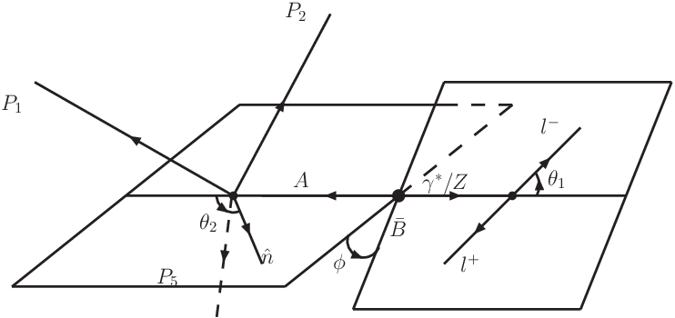
Before the results for these amplitudes are presented, we will give our convention on the helicity angles which are depicted in Fig. 6. Experimentally, the $K_{1}$ meson will be reconstructed by the three pseudoscalar state $K\pi\pi$ . In the rest frame of the $K_{1}$ meson, the final three mesons move in one decay plane and the direction normal to this decay plane is denoted as $\hat{n}$ . The angle between the direction $\hat{n}$ and the $K_{1}$ moving direction in the $B$ meson rest frame is defined as $\theta_{2}$ , while the angle between the moving direction of $l^{-}$ in the lepton pair rest frame and the moving direction of the lepton pair in the $B$ meson rest frame is defined as $\theta_{1}$ . The angle between the $l^{+}l^{-}$ decay plane and the plane defined by the $K_{1}$ moving direction in the $B$ meson rest frame and $\hat{n}$ is defined as $\phi$ .

In the rest frame of the lepton pair, the leptonic decay amplitudes are evaluated as

$\displaystyle{L}(L,0)$	$\displaystyle=$	$\displaystyle 2\sqrt{q^{2}}\sin\theta_{1},\;\;\;$	(41)
$\displaystyle{L}(L,+)$	$\displaystyle=$	$\displaystyle-2\sqrt{2}\sqrt{q^{2}}\sin^{2}\frac{\theta_{1}}{2}e^{i\phi},\;\;\;$	(42)
$\displaystyle{L}(L,-)$	$\displaystyle=$	$\displaystyle-2\sqrt{2}\sqrt{q^{2}}\cos^{2}\frac{\theta_{1}}{2}e^{-i\phi},$	(43)
$\displaystyle{L}(R,0)$	$\displaystyle=$	$\displaystyle-2\sqrt{q^{2}}\sin\theta_{1},\;\;\;$	(44)
$\displaystyle{L}(R,+)$	$\displaystyle=$	$\displaystyle-2\sqrt{2}\sqrt{q^{2}}\cos^{2}\frac{\theta_{1}}{2}e^{i\phi},\;\;\;$	(45)
$\displaystyle{L}(R,-)$	$\displaystyle=$	$\displaystyle-2\sqrt{2}\sqrt{q^{2}}\sin^{2}\frac{\theta_{1}}{2}e^{-i\phi}.$	(46)

In the $B$ meson rest frame, the hadronic transition amplitudes are given by

	$\displaystyle{H}(L,0)$	$\displaystyle=$	$\displaystyle\frac{G_{F}V_{tb}V^{*}_{ts}\alpha_{em}}{8\sqrt{2}\pi m_{A}\sqrt{q^{2}}}\bigg\{2(C_{7L}+C_{7R})m_{b}\left[\frac{\lambda T_{3}(q^{2})}{m_{B}^{2}-m_{A}^{2}}-\left(3m_{A}^{2}+m_{B}^{2}-q^{2}\right)T_{2}(q^{2})\right]$		(47)
			$\displaystyle+(C_{9}^{\rm eff}-C_{10})\left[(m_{B}-m_{A})(m_{A}^{2}-m_{B}^{2}+q^{2})V_{1}(q^{2})+\frac{\lambda V_{2}(q^{2})}{(m_{B}-m_{A})}\right]\bigg\},\;\;\;$		(47)

	$\displaystyle{H}(L,+)$	$\displaystyle=$	$\displaystyle\frac{G_{F}V_{tb}V^{*}_{ts}\alpha_{em}}{4\sqrt{2}\pi q^{2}}\bigg\{2(C_{7L}-C_{7R})m_{b}\sqrt{\lambda}T_{1}(q^{2})-2(C_{7L}+C_{7R})m_{b}(m_{B}^{2}-m_{A}^{2})T_{2}(q^{2})$		(48)
			$\displaystyle+(C_{9}^{\rm eff}-C_{10})q^{2}\bigg[\frac{\sqrt{\lambda}A(q^{2})}{(m_{B}-m_{A})}-(m_{B}-m_{A})V_{1}(q^{2})\bigg]\bigg\},\;\;\;$		(48)

	$\displaystyle{H}(L,-)$	$\displaystyle=$	$\displaystyle\frac{G_{F}V_{tb}V^{*}_{ts}\alpha_{em}}{4\sqrt{2}\pi q^{2}}\bigg\{-2(C_{7L}-C_{7R})m_{b}\sqrt{\lambda}T_{1}(q^{2})-2(C_{7L}+C_{7R})m_{b}(m_{B}^{2}-m_{A}^{2})T_{2}(q^{2})$		(49)
			$\displaystyle+(C_{9}^{\rm eff}-C_{10})q^{2}\bigg[-\frac{\sqrt{\lambda}A(q^{2})}{(m_{B}-m_{A})}-(m_{B}-m_{A})V_{1}(q^{2})\bigg]\bigg\},\;\;\;$		(49)

	$\displaystyle{H}(R,0)$	$\displaystyle=$	$\displaystyle\frac{G_{F}V_{tb}V^{*}_{ts}\alpha_{em}}{8\sqrt{2}\pi m_{A}\sqrt{q^{2}}}\bigg\{2(C_{7L}+C_{7R})m_{b}\left[\frac{\lambda T_{3}(q^{2})}{m_{B}^{2}-m_{A}^{2}}-\left(3m_{A}^{2}+m_{B}^{2}-q^{2}\right)T_{2}(q^{2})\right]$		(50)
			$\displaystyle+(C_{9}^{\rm eff}+C_{10})\left[(m_{B}-m_{A})(m_{A}^{2}-m_{B}^{2}+q^{2})V_{1}(q^{2})+\frac{\lambda V_{2}(q^{2})}{(m_{B}-m_{A})}\right]\bigg\},\;\;\;$		(50)

	$\displaystyle{H}(R,+)$	$\displaystyle=$	$\displaystyle\frac{G_{F}V_{tb}V^{*}_{ts}\alpha_{em}}{4\sqrt{2}\pi q^{2}}\bigg\{2(C_{7L}-C_{7R})m_{b}\sqrt{\lambda}T_{1}(q^{2})-2(C_{7L}+C_{7R})m_{b}(m_{B}^{2}-m_{A}^{2})T_{2}(q^{2})$		(51)
			$\displaystyle+(C_{9}^{\rm eff}+C_{10})q^{2}\bigg[\frac{\sqrt{\lambda}A(q^{2})}{(m_{B}-m_{A})}-(m_{B}-m_{A})V_{1}(q^{2})\bigg]\bigg\},\;\;\;$		(51)

	$\displaystyle{H}(R,-)$	$\displaystyle=$	$\displaystyle\frac{G_{F}V_{tb}V^{*}_{ts}\alpha_{em}}{4\sqrt{2}\pi q^{2}}\bigg\{-2(C_{7L}-C_{7R})m_{b}\sqrt{\lambda}T_{1}(q^{2})-2(C_{7L}+C_{7R})m_{b}(m_{B}^{2}-m_{A}^{2})T_{2}(q^{2})$		(52)
			$\displaystyle+(C_{9}^{\rm eff}+C_{10})q^{2}\bigg[-\frac{\sqrt{\lambda}A(q^{2})}{(m_{B}-m_{A})}-(m_{B}-m_{A})V_{1}(q^{2})\bigg]\bigg\}.\;\;\;$		(52)

References

[1] C. H. Chen, C. Q. Geng, Y. K. Hsiao and Z. T. Wei, Phys. Rev. D 72, 054011 (2005) [arXiv:hep-ph/0507012].
[2] H. Hatanaka and K. C. Yang, Phys. Rev. D 77, 094023 (2008) [Erratum-ibid. D 78, 059902 (2008)] [arXiv:0804.3198 [hep-ph]].
[3] M. J. Aslam, Eur. Phys. J. C 49, 651 (2007) [arXiv:hep-ph/0604025].
[4] M. Jamil Aslam and Riazuddin, Phys. Rev. D 72, 094019 (2005) [arXiv:hep-ph/0509082].
[5] V. Bashiry and K. Azizi, arXiv:0903.1505 [hep-ph].
[6] V. Bashiry, arXiv:0902.2578 [hep-ph].
[7] M. Bayar and K. Azizi, arXiv:0811.2692 [hep-ph].
[8] S. R. Choudhury, A. S. Cornell and N. Gaur, Eur. Phys. J. C 58, 251 (2008) [arXiv:0707.0446 [hep-ph]].
[9] M. A. Paracha, I. Ahmed and M. J. Aslam, Eur. Phys. J. C 52, 967 (2007) [arXiv:0707.0733 [hep-ph]].
[10] I. Ahmed, M. A. Paracha and M. J. Aslam, Eur. Phys. J. C 54, 591 (2008) [arXiv:0802.0740 [hep-ph]].
[11] A. Saddique, M. J. Aslam and C. D. Lu, Eur. Phys. J. C 56, 267 (2008) [arXiv:0803.0192 [hep-ph]].
[12] H. Hatanaka and K. C. Yang, Phys. Rev. D 78, 074007 (2008) [arXiv:0808.3731 [hep-ph]].
[13] B. B. Sirvanli, arXiv:0810.2677 [hep-ph].
[14] W. Wang, R. H. Li and C. D. Lu, arXiv:0711.0432 [hep-ph].
[15] R. H. Li, C. D. Lu and W. Wang, Phys. Rev. D 79, 034014 (2009).
[16] B. Aubert et al. [BABAR Collaboration], Phys. Rev. Lett. 97, 051802 (2006) [arXiv:hep-ex/0603050].
[17] K. Abe et al. [Belle Collaboration], arXiv:0706.3279 [hep-ex].
[18] G. Buchalla, A. J. Buras and M. E. Lautenbacher, Rev. Mod. Phys. 68, 1125 (1996) [arXiv:hep-ph/9512380].
[19] C. D. Lu and D. X. Zhang, Phys. Lett. B 397, 279 (1997) [arXiv:hep-ph/9702358].
[20] A. J. Buras and M. Munz, Phys. Rev. D 52, 186 (1995) [arXiv:hep-ph/9501281].
[21] Z. Ligeti and M. B. Wise, Phys. Rev. D 53, 4937 (1996) [arXiv:hep-ph/9512225].
[22] C. Amsler et al. [Particle Data Group], Phys. Lett. B 667, 1 (2008).
[23] K. C. Yang, Nucl. Phys. B 776, 187 (2007) [arXiv:0705.0692 [hep-ph]].
[24] S. M. Berman and M. Jacob, Phys. Rev. 139, B1023 (1965).
[25] A. Datta, Y. Gao, A. V. Gritsan, D. London, M. Nagashima and A. Szynkman, Phys. Rev. D 77, 114025 (2008) [arXiv:0711.2107 [hep-ph]].

$\displaystyle\frac{d^{4}\Gamma}{dq^{2}d\cos\theta_{1}d\cos\theta_{2}d\phi}$	$\displaystyle\propto$	$\displaystyle\frac{1}{\sum_{m}\|R_{m}\|^{2}}\sum_{m}\|R_{m}\|^{2}\left[\left\|\sum_{\lambda}H(L,\lambda)L(L,\lambda)d_{\lambda,m}^{J_{2}}(\theta_{2})\right\|^{2}+\left\|\sum_{\lambda}H(R,\lambda)L(R,\lambda)d_{\lambda,m}^{J_{2}}(\theta_{2})\right\|^{2}\right]$	(22)
	$\displaystyle=$	$\displaystyle 2q^{2}\bigg\{2\big(\|H(L,0)\|^{2}+\|H(R,0)\|^{2})\big)\sin^{2}\theta_{1}\sin^{2}\theta_{2}$
		$\displaystyle+\frac{\|H(L,1)\|^{2}+\|H(R,-1)\|^{2}}{2}(1-\cos\theta_{1})^{2}(1+\cos^{2}\theta_{2})$
		$\displaystyle+\frac{\|H(L,-1)\|^{2}+\|H(R,1)\|^{2}}{2}(1+\cos\theta_{1})^{2}(1+\cos^{2}\theta_{2})$
		$\displaystyle+{\rm Re}\big[H(L,0)H(L,1)^{}+H(R,0)H(R,-1)^{}\big](1-\cos\theta_{1})(1+\cos\theta_{2})\sin\theta_{1}\sin\theta_{2}\cos\phi$
		$\displaystyle+{\rm Im}\big[H(L,0)H(L,1)^{}+H(R,0)^{}H(R,-1)\big](1-\cos\theta_{1})(1+\cos\theta_{2})\sin\theta_{1}\sin\theta_{2}\sin\phi$
		$\displaystyle+{\rm Re}\big[H(L,0)H(L,-1)^{}+H(R,0)H(R,1)^{}\big](1+\cos\theta_{1})(1-\cos\theta_{2})\sin\theta_{1}\sin\theta_{2}\cos\phi$
		$\displaystyle+{\rm Im}\big[H(L,0)^{}H(L,-1)+H(R,0)H(R,1)^{}\big](1+\cos\theta_{1})(1-\cos\theta_{2})\sin\theta_{1}\sin\theta_{2}\sin\phi$
		$\displaystyle+{\rm Re}\big[H(L,1)H(L,-1)^{}+H(R,1)H(R,-1)^{}\big]\sin^{2}\theta_{1}\sin^{2}\theta_{2}\cos(2\phi)$
		$\displaystyle+{\rm Im}\big[H(L,1)^{}H(L,-1)+H(R,1)^{}H(R,-1)\big]\sin^{2}\theta_{1}\sin^{2}\theta_{2}\sin(2\phi)$
		$\displaystyle-{\rm Re}\big[H(R,0)H(R,1)^{}+H(L,0)H(L,-1)^{}\big](1+\cos\theta_{1})(1+\cos\theta_{2})\sin\theta_{1}\sin\theta_{2}\cos\phi$
		$\displaystyle-{\rm Im}\big[H(R,0)H(R,1)^{}+H(L,0)^{}H(L,-1)\big](1+\cos\theta_{1})(1+\cos\theta_{2})\sin\theta_{1}\sin\theta_{2}\sin\phi$
		$\displaystyle-{\rm Re}\big[H(R,0)H(R,-1)^{}+H(L,0)H(L,1)^{}\big](1-\cos\theta_{1})(1-\cos\theta_{2})\sin\theta_{1}\sin\theta_{2}\cos\phi$
		$\displaystyle-{\rm Im}\big[H(R,0)^{}H(R,-1)+H(L,0)H(L,1)^{}\big](1-\cos\theta_{1})(1-\cos\theta_{2})\sin\theta_{1}\sin\theta_{2}\sin\phi\bigg\}$
		$\displaystyle+2q^{2}r_{1}\bigg\{({\|H(L,1)\|^{2}-\|H(R,-1)\|^{2}})(1-\cos\theta_{1})^{2}\cos\theta_{2}$
		$\displaystyle+({\|H(R,1)\|^{2}-\|H(L,-1)\|^{2}})(1+\cos\theta_{1})^{2}\cos\theta_{2}$
		$\displaystyle+{\rm Re}\big[H(L,0)H(L,1)^{}-H(R,0)H(R,-1)^{}\big](1-\cos\theta_{1})(1+\cos\theta_{2})\sin\theta_{1}\sin\theta_{2}\cos\phi$
		$\displaystyle+{\rm Im}\big[H(L,0)H(L,1)^{}-H(R,0)^{}H(R,-1)\big](1-\cos\theta_{1})(1+\cos\theta_{2})\sin\theta_{1}\sin\theta_{2}\sin\phi$
		$\displaystyle+{\rm Re}\big[H(L,0)H(L,-1)^{}-H(R,0)H(R,1)^{}\big](1+\cos\theta_{1})(1-\cos\theta_{2})\sin\theta_{1}\sin\theta_{2}\cos\phi$
		$\displaystyle+{\rm Im}\big[H(L,0)^{}H(L,-1)-H(R,0)H(R,1)^{}\big](1+\cos\theta_{1})(1-\cos\theta_{2})\sin\theta_{1}\sin\theta_{2}\sin\phi$
		$\displaystyle-{\rm Re}\big[H(R,0)H(R,1)^{}-H(L,0)H(L,-1)^{}\big](1+\cos\theta_{1})(1+\cos\theta_{2})\sin\theta_{1}\sin\theta_{2}\cos\phi$
		$\displaystyle-{\rm Im}\big[H(R,0)H(R,1)^{}-H(L,0)^{}H(L,-1)\big](1+\cos\theta_{1})(1+\cos\theta_{2})\sin\theta_{1}\sin\theta_{2}\sin\phi$
		$\displaystyle-{\rm Re}\big[H(R,0)H(R,-1)^{}-H(L,0)H(L,1)^{}\big](1-\cos\theta_{1})(1-\cos\theta_{2})\sin\theta_{1}\sin\theta_{2}\cos\phi$
		$\displaystyle-{\rm Im}\big[H(R,0)^{}H(R,-1)-H(L,0)H(L,1)^{}\big](1-\cos\theta_{1})(1-\cos\theta_{2})\sin\theta_{1}\sin\theta_{2}\sin\phi\bigg\},$

Branching Ratios, Forward-backward Asymmetry and Angular Distributions of B→K1​l+​l−B\to K_{1}l^{+}l^{-} Decays