May, 2008
A short introduction to Fibonacci anyon models
Abstract
We discuss how to construct models of interacting anyons by generalizing quantum spin Hamiltonians to anyonic degrees of freedom. The simplest interactions energetically favor pairs of anyons to fuse into the trivial (“identity”) channel, similar to the quantum Heisenberg model favoring pairs of spins to form spin singlets. We present an introduction to the theory of anyons and discuss in detail how basis sets and matrix representations of the interaction terms can be obtained, using non-Abelian Fibonacci anyons as example. Besides discussing the “golden chain”, a one-dimensional system of anyons with nearest neighbor interactions, we also present the derivation of more complicated interaction terms, such as three-anyon interactions in the spirit of the Majumdar-Ghosh spin chain, longer range interactions and two-leg ladders. We also discuss generalizations to anyons with general non-Abelian SU(2)k statistics. The limit of the latter yields ordinary SU(2) spin chains.
1 Introduction
While in classical mechanics the exchange of two identical particles does not change the underlying state, quantum mechanics allows for more complex behavior. In three-dimensional quantum systems the exchange of two identical particles may result in a sign-change of the wavefunction which distinguishes fermions from bosons. Two-dimensional quantum systems – such as electrons confined between layers of semiconductors – can give rise to exotic particle statistics, where the exchange of two identical (quasi)particles can in general be described by either Abelian or non-Abelian statistics. In the former, the exchange of two particles gives rise to a complex phase , where correspond to the statistics of bosons and fermions, respectively, and is referred to as the statistics of Abelian anyons. The statistics of non-Abelian anyons are described by unitary matrices acting on a degenerate ground-state manifold with . In general, two such unitary matrices do not necessarily commute, i.e. , or in more mathematical language, the unitary matrices form a non-Abelian group when , hence the term non-Abelian anyons.
Anyons appear as emergent quasiparticles in fractional quantum Hall states and as excitations in microscopic models of frustrated quantum magnets that harbor topological quantum liquids [1, 2, 3]. While for most quantum Hall states the exchange statistics is Abelian, there are quantum Hall states at certain filling fractions, e.g. and , for which non-Abelian quasiparticle statistics have been proposed [4, 5], namely those of so-called Ising anyons [6] and Fibonacci anyons [7] respectively. Non-Abelian anyons have also generated considerable interest in proposals for topological quantum computation [8], where braiding of anyons is used to perform the unitary transformations of a quantum computation. The simplest anyons with non-Abelian braiding statistics that can give rise to universal quantum computation11 1 Roughly speaking, a universal quantum computer is a general-purpose quantum computer which is capable of simulating any program on another quantum computer. are the so-called Fibonacci anyons which we will discuss in detail in this manuscript.
In the following, we will first give a short introduction to the mathematical theory of anyons, and discuss how to (consistently) describe the degenerate manifold of a set of (non-interacting) anyons. Having established the basic formalism we will then turn to the question of how to model interactions between anyons and explicitly construct matrix representations of generalized quantum spin Hamiltonians. We then discuss an alternative formulation in terms of non-Abelian SU(2)k anyons. Rounding off the manuscript, we shortly review some recent work analyzing the ground-state phase diagrams of these Hamiltonians.
2 Basic theory
2.1 Algebraic theory of anyons
In general terms, we can describe anyons by a mathematical framework called tensor category theory. In such a categorical description, anyons are simple objects in the corresponding tensor categories, and anyon types are the isomorphism classes of anyons. Here we will not delve into this difficult mathematical subject, but focus on the theory of Fibonacci anyons, where many simplifications occur.
2.2 Particle types and fusion rules
To describe a system of anyons, we list the species of the anyons in the system, also called the particle types or topological charges or simply labels (and many other names); we also specify the anti-particle type of each particle type. We will list the particle types as , and use to denote a representative set of anyons, where the type of is .
In any anyonic system, we always have a trivial particle type denoted by , which represents the ground states of the system or the vacuum. In the list of particle types above, we assume . The trivial particle is its own anti-particle. The anti-particle of , denoted as , is always of the type of another . If and are of the same type, we say is self-dual.
To have a non-trivial anyonic system, we need at least one more particle type besides . The Fibonacci anyonic system is such an anyonic system with only two particle types: the trivial type , and the nontrivial type . Anyons of type are called the Fibonacci anyons. Fibonacci anyons are self-dual: the anti-particle type of is also . Strictly speaking, we need to distinguish between anyons and their types. For Fibonacci anyons, this distinction is unnecessary. Therefore, we will refer to both as an anyon and its type, and no confusion should arise.
Anyons can be combined in a process called the fusion of anyons, which is similar to combining two quantum spins to form a new total spin. Repeated fusions of the same two anyons do not necessarily result in an anyon of the same type: the resulting anyons may be of several different types each with certain probabilities (determined by the theory). In this sense we can also think of fusion as a measurement. It follows that given two anyons of type , the particle type of the fusion, denoted as , is in general not well-defined.
Given an anyon , if the fusion of with any other anyon (maybe itself) always produces an anyon of the same type, then is called an Abelian anyon. If neither nor is Abelian, then there will be anyons of more than one type as the possible fusion results. When such fusion occurs, we say that the fusion has multi-fusion channels.
Given two anyons , we formally write the fusion result as , where are all anyons in a representative set, and are non-negative integers. The non-negative integer is called the multiplicity of the occurrence of anyon . Multi-fusion channels correspond to . Given an anyonic system with anyon representative set , then we have , or equivalently, . The non-negative integers are called the fusion rules of the anyonic system. If , we say the fusion of and to is admissible.
The trivial particle is Abelian as the fusion of the trivial particle with any other particle does not change the type of , i.e., for any type .
For the Fibonacci anyonic system the particle types are denoted as and , and the fusion rules are given by:
where the denotes the two possible fusion channels.
2.3 Many anyon states and fusion tree basis
A defining feature of non-Abelian anyons is the existence of multi-fusion channels. Suppose we have three anyons localized in the plane, well-separated, and numbered as . We would like to know when all three anyons are brought together to fuse, what kinds of anyons will this fusion result in? When anyons and are combined, we may see or . If the resulting anyon were , then after combining with the third , we would have a anyon. If the resulting anyon were , then fusion with the third anyon would result in either or . Hence the fusion result is not unique. Moreover, even if we fix the resulting outcome as , there are still two possible fusion paths: the first two ’s were fused to , then fused with the third to , or the first two ’s were fused to , then fused with the third to . Each such fusion path will be recorded by a graphical notation of the fusion tree, see Fig. 1.

A fusion path is a labeling of the fusion tree where each edge is labeled by a particle type, and the three labels around any trivalent vertex represent a fusion admissible by the fusion rules. If not all particles are self-dual, then the edges of the fusion tree should be oriented. We always draw anyons to be fused on a straight line, and the fusion tree goes downward. The top edges are labeled by the anyons to be fused, and the bottom edge represents the fusion result and is also called the total charge of the fused anyons.
In general, given -anyons in the plane localized at certain well separated places, we will assume the total charge at the boundary is either or . In theory any superposition of or is possible for the total charge, but it is physically reasonable to assume that such superpositions will decohere into a particular anyon if left alone. Let us arrange the anyons on the real axis of the plane, numbered as . When we fuse the anyons consecutively, we have a fusion tree as below:
![[Uncaptioned image]](0902.3275v1/FusionTree.png)
The ground-state manifold of a multi-anyon system in the plane even when the positions of the anyons are fixed might be degenerate: there is more than one ground state (in reality the energy differences between the different ground states go to exponentially as the anyon separations go to infinity; we will ignore such considerations here, and always assume that anyons are well separated until they are brought together for fusion.) Such a degeneracy is in fact necessary for non-Abelian statistics to occur. How can we describe a basis for this degenerate ground state manifold?
As we see in the example of three anyons, there are multi-fusion paths, which are represented by labelings of the fusion tree. We claim that these fusion paths represent an orthonormal basis of the degenerate ground-state manifold.22 2 We will not further justify this assertion, but mention that in the conformal field theory (CFT) description of fractional quantum Hall liquids the ground states can be described by conformal blocks, which form a basis of the modular functor. Conformal blocks are known to be represented by labeled fusion trees, which we refer to as fusion paths.
The fusion tree basis of a multi-anyon system then leads to a combinatorial way to compute the degeneracy: count the number of labelings of the fusion tree or equivalently the number of fusion paths. Consider -anyons in the plane with total charge , and denote the ground state degeneracy as . Simple counting shows that and . Easy induction then gives . This is exactly the Fibonacci sequence, hence the name of Fibonacci anyons.
As alluded to above, when two anyons are fused, and each occurs with a certain probability. This probability is given by the so-called quantum dimension of an anyon. Consider the fusion coefficients of a theory, if we regard the particle types as variables and the fusion rules as equations for . Then in a unitary theory the solutions of which are are the quantum dimensions of the anyons of type . is also the Perron-Frobenius eigenvalue of the matrix whose th entry is . We also introduce the total quantum order . The quantum dimension of the trivial type is always . In the Fibonacci theory, the quantum dimension of is the golden ratio . When two anyons fuse, the probability to see is , and the probability to see is .
2.4 F-matrices and pentagons
In the discussion of the fusion tree basis above, we fuse the anyons consecutively one by one from left to right, e.g., gives the left fusion tree below. We may as well choose any other order for the fusions. For example, in the case of three ’s with total charge , we may first fuse the second and third ’s, then fuse the resulting anyon with the first . This will lead to the fusion tree on the right as shown in Fig. 2.

Given anyons with a certain total charge, then each order of the fusions is represented by a fusion tree, and the admissible labelings of the respective fusion trees each constitute a basis of the multi-anyon system.
The change from the left fusion tree to the right fusion tree in Fig. 2 is called the -move. Since both fusion tree bases describe the same degenerate ground state manifold of anyons with a certain total charge, they should be related by a unitary transformation. The associated unitary matrix is called the -matrix. The -matrix will be denoted as , where are the anyons to be fused, and is the resulting anyon or total charge (Complications from fusion coefficients are ignored.)
For more than three anyons, there will be many more different fusion trees. To have a consistent theory, a priori we need to specify the change of basis matrices for any number of anyons in a consistent way: for example as shown in Fig. 3 the left-most and right-most fusion trees of four anyons can be related to each other by -moves in two different sequences of applications of -moves.

Fortunately, a mathematical theorem guarantees that the consistency equations for the above fusion trees, called the pentagons, are all the equations that need to be satisfied, i.e., all other consistencies are consequences of the pentagons. Note that the pentagons are just polynomial equations for the entries of the -matrices.
To set up the pentagons, we need to explain the consistency of fusion tree bases for any number of anyons. Consider a fusion tree , and a decomposition of into two sub-fusion trees by cutting an edge; the resulting new edge of will also be referred to as edge . The fusion tree basis for has a corresponding decomposition: if ’s are the particle types of the theory (we assume they are all self-dual), for each , we have a fusion tree basis for with the edge labeled by . Then the fusion tree basis of is the direct sum over all of the tensor product: (the fusion tree basis of ) (the fusion tree basis of ).
In the pentagons, an -move is applied to part of the fusion trees in each step. The fusion tree decomposes into two pieces: the part where the -move applies, and the remaining part. It follows that the fusion tree basis decomposes as a direct sum of two terms: corresponding to and .
Given a set of fusion rules solving the pentagons turns out to be a difficult task (even with the help of computers). However, certain normalizations can be made to simplify the solutions. If one of the indices of the -matrix is the trivial type , we may assume . In the Fibonacci theory, we may also assume . It follows that the only non-trivial -matrix is , which is a unitary matrix.
There are many pentagons even for the Fibonacci theory depending on the four anyons to be fused and their total charges: a priori . It is easy to see that the only non-trivial pentagon for is the one with ’s at all outer edges. The pentagon is a matrix equation for extended to a bigger Hilbert space. To write down the pentagon, we need to order the fusion tree basis with respect to the decomposition above carefully.
Written explicitly for Fibonacci anyons the pentagon equation reads
| (1) |
where the indices label the inner edges of the fusion tree as shown in Fig. 3. There are only a few different matrices appearing, of which four are uniquely determined by the fusion rules
| (2) |
in a basis for the labeling on the central edge. The only nontrivial matrix is . Setting the pentagon equation simplifies to
| (3) |
which combined with the condition that is unitary constrains the matrix, up to arbitrary phases, to be
| (4) |
where is the golden ratio.
2.5 R-matrix and hexagons
Given anyons in a surface , well-separated at fixed locations , we may consider the ground states of this quantum system. Since an energy gap in an anyonic system is always assumed, if two well-separated anyons are exchanged slowly enough, the system will remain in the ground states manifold . If is the initial ground state, then after the exchange, or the braiding of the two anyons in mathematical parlor, the system will be in another ground state in , where is an othonormal basis of the ground states manifold . When runs over the basis , we obtain a unitary matrix from to itself. In mathematical terms, we obtain a representation of the mapping class group of the punctured surface . If is the disk, the mapping class group is called the braid group. In a nice basis of , the braiding matrix becomes diagonal.
To describe braidings carefully, we introduce some conventions. When we exchange two anyons in the plane, there are two different exchanges which are not topologically equivalent: their world lines are given by the following two pictures, which are called braids mathematically. In our convention time goes upwards. When we exchange two anyons, we will refer to the right process, which is called the right-handed braiding. The left process is the inverse, left-handed braiding.
![[Uncaptioned image]](0902.3275v1/Braiding1.png)
Now a comment about fusion trees is necessary. In our convention, we draw the fusion trees downwards. If we want to interpret a fusion tree as a physical process in time, we should also introduce the conjugate operator of the fusion: splitting of anyons from one to two. Then as time goes upwards, a fusion tree can be interpreted as a splitting of one anyon into many.
All the braiding matrices can be obtained from the -matrices combined with -matrices. Let be the ground state manifold of two anyons of types with total charge . Let us assume all spaces are one-dimensional, and be its fusion tree basis.
When anyons and are braided by , the state in is changed into a state in . Since both and are non-zero vectors in a one-dimensional Hilbert space , they are equal up to a phase, denoted as , i.e, . Here, is a phase, but in general, is a unitary matrix. We should mention that in general is not the inverse of . Their product involves the twists of particles.
![[Uncaptioned image]](0902.3275v1/Braiding2.png)
As we have seen before anyons can be fused or splitted, therefore braidings should be compatible with them. For example, given two anyons , we may first split to , then braid with followed by braid with , or we may braid and first, then split into . These two processes are physically equivalent, therefore their resulting matrices should be the same. Applying the two operators on the fusion tree basis , we have an identity in pictures:
![[Uncaptioned image]](0902.3275v1/Braiding4.png)

The same identity can be also obtained as a composition of -moves and braidings as shown in Fig. 4. It follows the composition of the matrices, hence the name hexagon, should be the same as the identity. The resulting equations are called hexagons. There is another family of hexagons obtained by replacing all right-handed braids with left-handed ones. In general, these two families of hexagons are independent of each other. Similar to the pentagons, a mathematical theorem says that the hexagons imply all other consistency equations for braidings.
Written explicitly for Fibonacci anyons the hexagon equation reads
| (5) |
where again the indices label the internal edges of the fusion trees as shown in Fig. 4. Inserting the -matrix (4) and realizing that braiding a particle around the trivial one is trivial: the hexagon equation becomes
| (6) |
which has the solution
| (7) |
The combined operation of a basis transformation before applying the -matrix is often denoted by the braid-matrix
| (8) |
Using a basis for the labelings adjacent to the two anyons to be braided the basis before the basis transformation is
| (9) |
and after the basis change to a basis using an matrix the basis is
| (10) |
as illustrated here.
![[Uncaptioned image]](0902.3275v1/BraidBasisTransformation.png)
In this representation the -matrix is given by
| (11) |
and the -matrix is
| (12) |
We finally obtain for the braid matrix
| (13) |
With the explicit matrix representations of the basis transformation and the braid matrix , we are now fully equipped to derive matrix representations of Hamiltonians describing interactions between Fibonacci anyons.
3 Hamiltonians
Considering a set of Fibonacci anyons we will now address how to model interactions between these anyons. Without any interactions, the collective state of the anyons will simply be described by the large degenerate manifold described by the Hilbert space introduced above. If, however, the anyons interact, this degeneracy will be split and a non-trivial collective ground state is formed. In this section we will first motivate a particular type of interaction, which generalizes the well-known Heisenberg exchange interaction to anyonic degrees of freedom, and then explicitly derive various Hamiltonians of interacting Fibonacci anyons that correspond to well-known models of SU(2) spin-1/2’s.
Two SU(2) spin-1/2’s can be combined to form a total spin singlet or a total spin triplet , which in analogy to the anyonic fusion rules we might write as
If the two spins are far apart and interact only weakly, these two states are degenerate. However, if we bring the two spins close together a strong exchange will be mediated by a virtual tunneling process and the degeneracy between the two total spin states will be lifted. This physics is captured by the Heisenberg Hamiltonian which for SU(2) spins is given by
| (14) |
where and are SU(2) spin 1/2’s, is the total spin formed by the two spins and , a (uniform) coupling constant is denoted as , and the sum runs over all pairs of spins (or might be restricted to nearest neighbors on a given lattice). Of course, the Heisenberg Hamiltonian is just a sum of projectors onto the pairwise spin singlet state as can be easily seen by rewriting the spin exchange in terms of the total spin . Antiferromagnetic coupling () favors an overall singlet state (), while a ferromagnet coupling () favors the triplet state ().

In analogy, we can consider two Fibonacci anyons. If the two anyons are far apart and weakly or non-interacting, then the two states that can be formed by fusing the two anyons will be degenerate. If, however, the anyons interact more strongly, then it is natural to assume that the two fusion outcomes will no longer be degenerate and one of them is energetically favored. We can thus generalize the Heisenberg Hamiltonian to anyonic degrees of freedom by expressing it as a sum of projectors onto a given fusion outcome
| (15) |
where is a projector onto the trivial channel.
3.1 The golden chain
We will now explicitly derive the matrix representations for simple models of interacting Fibonacci anyons. In the simplest model we consider a chain of Fibonacci anyons with nearest neighbor Heisenberg interactions as shown in Fig. 6.

This Hamiltonian favors neighboring anyons to fuse into the trivial (1) channel by assigning an energy to that fusion outcome. To derive the matrix representation in the fusion tree basis we first need to perform a basis change using the -matrix
![[Uncaptioned image]](0902.3275v1/GoldenChainBasisTransformation.png)
3.2 Three-anyon fusion
For the second model we include longer range interactions, preferring now to fuse three adjacent anyons into the trivial particle. For this we have to perform two basis changes to obtain the total charge of three anyons as shown here:
![[Uncaptioned image]](0902.3275v1/J3ChainBasisTransformation.png)
The basis states of three anyons are given by the labelings of the four edges between and adjacent to the three anyons:
| (18) |
The first matrix is
| (19) |
changing to the basis
| (20) |
and then a second basis change with
| (21) |
to a basis
| (22) |
Combined with the projector the Hamiltonian matrix then becomes
| (23) |
3.3 Next-nearest neighbor interactions
Another possibility for longer-range interactions is to fuse two particles at larger distance. Here we consider the case of next-nearest neighbor interactions. To determine the fusion result of these two anyons we first need to bring them to adjacent positions by braiding one of the particles with its neighbor as shown here:
![[Uncaptioned image]](0902.3275v1/J2ChainBraiding1.png)
In contrast to Abelian particles, such as ordinary spins, for non-Abelian anyons it matters whether we braid the two anyons clockwise or counter-clockwise, since the braid matrix (for braiding clockwise) is different from its inverse (braiding anti-clockwise). Indicating the interaction of two anyons by loops around the two, the two ways of braiding correspond to the anyons fusing above or below the one between then as shown here:
![[Uncaptioned image]](0902.3275v1/J2ChainBraiding2.png)
Using the same basis as above we obtain for the Hamiltonian for upper and lower interactions
| (24) | |||
and
| (34) |
where is the braid matrix acting on the first two anyone (first three labels) and . For the symmetrized model containing both terms we have
| (35) | |||
As for SU(2) spin chains, the three-particle interaction can be written as a sum of nearest and next-nearest neighbor terms: For SU(2) spin-S this is
| (45) | |||||
where the indicates a nearest neighbor interaction between sites and and a next-nearest neighbor one. Mapping an chain to a chain containing both and terms we find and . The chain thus corresponds to the Majumdar-Ghosh chain [9] with an exact ground state of singlet dimers.
Similarly we find for Fibonacci anyons
| (46) |
and thus and . Again the pure chain corresponds to the Majumdar-Ghosh chain with an exact ground state of anyonic dimers fusing into the trivial particle [10].
Generalizations of the next nearest neighbor interaction to longer distances is straightforward, the only complication arises from the various possible orientations of the braids, giving different terms at distance .
3.4 The two-leg ladder
The final model we will present is a two-leg ladder consisting of two coupled chains. Unlike the case of the chain, where it was natural to just use the standard fusion tree as basis, there are several natural choices here. Choosing the zig-zag fusion path indicated by a line in Fig. 7 minimizes the interaction range on the fusion tree.

Distinguishing rung interactions with coupling constant and chain interactions with coupling , we see that the rung terms are just nearest neighbor interactions and the chain terms are next nearest neighbor interactions above or below the other anyon for the upper and lower chain respectively:
| (47) |
Having established the explicit matrix representations of these Hamiltonians we can now analyze their ground states thereby addressing the original question of what kind of collective ground states a set of Fibonacci anyons will form in the presence of these interactions.
4 Alternative SU(2)k formulation
Before turning to the collective ground states of the Hamiltonians introduced above, we will describe an alternative reformulation of the “golden chain”, Eq. (15), which allows us to generalize the latter and, in particular, allows us to view the golden chain and its variants as certain deformations of ordinary SU(2) spin chains. Technically, this generalization is based on connections with the famous work by V. F. R. Jones [13] on representations of the Temperley-Lieb algebra [14].
Specifically, this reformulation is based on the fusion rules of the anyon theory known by the name ‘SU(2) at level ’, which in symbols we denote as SU(2)k, for . For arbitrary integer values of the parameter there exist particles labeled by ‘angular momenta’ . The result of fusing two particles with ‘angular momenta’ and yields particles with ‘angular momenta’ where , each occuring with multiplicity . When this represents ordinary SU(2) spins, for which all possible values of (ordinary) SU(2) angular momenta appear, and the fusion rule turns into the ordinary angular momentum coupling rule. Finite values of represent a ‘quantization’ of SU(2), amounting to the indicated truncation of the range of ‘angular momenta’. Thus, our reformulation will allow us to view the “golden chain” as a deformation of the ordinary SU(2) Heisenberg spin chain by a parameter . For the special case where we obtain, as we will now briefly review, the chain of Fibonacci anyons introduced in Eq. (15) above.
Our reformulation of the “golden chain” is based on two simple observations: (i) first, one recalls that at (where the four particles exist) the fusion rule of the particle with is (all entries label ‘angular momenta’), which is identical to that of the Fibonacci anyon , e.g. . Note that the trivial particle, previously denoted by , is now denoted by ‘angular momentum’ . (ii) Secondly, we recall that the particle can be used to map the particles one-to-one into each other (it represents what is known as an automorphism of the fusion algebra), i.e.
| (48) |
We denote this automorphism by
| (49) |
Note that when is an integer, then is a half-integer, and vice-versa.
Using the observation (i) above we may first write an arbitrary state vector in the Hilbert space which can be represented pictorially as
![[Uncaptioned image]](0902.3275v1/WaveFunction1.png)
,
in the new notation using the ’angular momenta’ as follows
![[Uncaptioned image]](0902.3275v1/WaveFunction2.png)
.

Let us now consider the matrix element of the projector [discussed in Eq.s (15) -(17) above]
| (50) |
where . A moment’s reflection shows that in fact and . This matrix element is graphically depicted in the leftmost picture in Fig. 8, where the direction from the right (ket) to the left (bra) in (50) is now drawn vertically upwards from bottom to top in the Figure.
We may now perform a number of elementary steps using a -dimensional -matrix (which is just a number) involving the Abelian particle . Specifically, we perform the steps depicted as
![[Uncaptioned image]](0902.3275v1/Transformation1.png)
on both, the upper and the lower legs of the projector in Fig. 8, where in the last step we use
![[Uncaptioned image]](0902.3275v1/Transformation2.png)
Subsequently we use, in the diagram in the middle of the projector equation Fig. 8, the transformation
![[Uncaptioned image]](0902.3275v1/Transformation3.png)
where in the first step we have applied the relation
![[Uncaptioned image]](0902.3275v1/Transformation4.png)
The projector with four particle legs (depicted in the rightmost diagram of Fig. 8), which we obtain at the end of this sequence of elementary steps is the central object of interest to us.
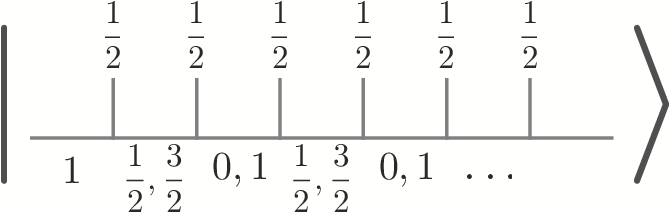
As it is evident from the rightmost picture in Fig. 8, the projector acts on basis states of the form
| (51) |
that is on states in which integer and half-integer labels are strictly alternating. Such basis states can then be depicted as
.
The projector that we have thereby obtained is a central and well known object of study in Mathematics: Specifically, let us form the operator
| (52) |
where is the golden ratio. The index indicates the label along the fusion chain basis of ‘angular momenta’ in (51) on which it acts. For example, the operator in (50) as drawn in Fig. 8 acts on the label which is, say, in the position in the chain of symbols characterizing the state. With these notations, the operators are known to provide a representation of the Temperley-Lieb algebra [14]
with -isotopy parameter . The so-obtained representation of the Temperley-Lieb algebra is only one in an infinite sequence with different values of the -isotopy parameter, discovered by V. F. R. Jones[13]. Specifically, in our notations, this infinite sequence is labeled by the integer , specifying the -isotopy parameter . For any integer value of , the Jones representation is given by the matrix elements of the operator in the basis of type (51). Recall from the discussion at the beginning of this paragraph that for general values of the integer the labels are the ‘angular momenta’ in the set . Thus it is in general more convenient to write these basis states as
| (53) |
with ; the sequence must satisfy the condition that is contained in the fusion product of with an ‘angular momentum’ , is contained in the fusion product of with ‘angular momentum’ , etc. – this generalizes the states depicted in Fig. 9 (which is written for ). Within this notation the matrix elements of the operator are (compare 50)
| (54) |
where
| (55) |
This, then, defines a generalization of the original “golden chain”, for which , to arbitrary values of . It is interesting to note that in the limit , the so-defined generalized anyonic chain turns precisely into the ordinary SU(2) spin-1/2 Heisenberg chain. Therefore, these generalized “golden chains” (for arbirary integer values of ) provide, as alluded to in the introduction of this section, a certain generalization of the ordinary SU(2) spin-1/2 Heisenberg chain. Therefore, it is natural to ask questions about the behavior of ordinary spin-1/2 chains, in the context of these generalized golden chains. Indeed, as we have described in various publications [11, 10, 12] and as reviewed in this note, many of the physics questions familiar from the ordinary Heisenberg chain find their mirror-image in the behavior of our generalized golden chains. The following section is intended to give a brief flavor of these results and parallels.
Before we proceed, let us briefly mention that for ‘antiferromagnetic’ coupling of the generalized spins of the golden chain (for general ), meaning that projection onto the singlet state (trivial anyon fusion channel) between two spins is energetically favored, one obtains a gapless theory which turns out to be precisely the -th minimal model of conformal field theory[15] of central charge . (For this is the Ising model, for the tricritical Ising model, and so on.) In the opposite, ‘ferromagnetic’ case, meaning the case where the projection onto the ‘generalized triplet’ state of two neighboring generalized spins is energetically favored, one obtains another well known sequence of gapless models: these are the parafermionic conformal field theories[16], of central charge , which have more recently attracted attention in quantum Hall physics as potential candidates for certain non-Abelian quantum Hall states, known as the Read-Rezayi states [5]. For a summary see Table I.
| level | AFM | FM |
|---|---|---|
| 2 | ||
| Ising | Ising | |
| 3 | ||
| tricritical Ising | 3-state Potts | |
| 4 | ||
| tetracritical Ising | -parafermions | |
| 5 | ||
| pentacritical Ising | -parafermions | |
| -multicritical Ising | -parafermions | |
| Heisenberg AFM | Heisenberg FM |
5 Collective ground states
In this final section we will round off the manuscript by shortly reviewing some recent numerical and analytical work analyzing the collective ground states formed by a set of Fibonacci anyons in the presence of the generalized Heisenberg interactions introduced in the previous section.
For the “golden chain” investigated in Ref. \citenGoldenChain , a one-dimensional arrangement of Fibonacci anyons with nearest neighbor interaction terms, it has been shown (as already mentioned above) that the system is gapless – independent of which fusion channel, the trivial channel () for antiferromagnetic coupling, or the -channel for ferromagnetic coupling, is energetically favored by the pairwise fusion. The finite-size gap for a system with Fibonacci anyons vanishes as with dynamical critical exponent , indicative of a conformally invariant energy spectrum. The two-dimensional conformal field theories describing the system have central charge for antiferromagnetic interactions and for ferromagnetic interactions, respectively, corresponding to the entry for in Table I. In fact, a direct connection to the corresponding two-dimensional classical models, the tricritical Ising model for and the three-state Potts model for , has been made: Realizing that (as reviewed briefly in the previous section) the non-commuting local operators of the “golden chain” Hamiltonian form a well known representation[13] of the Temperley-Lieb algebra[14] (with -isotopy parameter ), it has been shown[11] that the Hamiltonian of this quantum chain corresponds precisely to (a strongly anisotropic version of) the transfer matrix of the integrable restricted-solid-on-solid (RSOS) lattice model[17], thereby mapping the anyonic quantum chain exactly onto the tricritical Ising and three-state Potts critical points of the generalized hard hexagon model [11, 18]. A corresponding exact relationship holds in fact true for the chains at any value of the integer (Table I).

While this correspondence of the “golden chain” with the special critical points of the classical models might initially seem accidental, it turns out that the quantum system exhibits in fact an additional topological symmetry that actually stabilizes the gaplessness of the quantum system, and protects it from local perturbations which would generate a gap. In particular, it was shown that all translational-invariant relevant operators that appear in the quantum system, e.g. the two thermal operators of the tricritical Ising model (antiferromagnetic case) with scaling dimensions and respectively, are forbidden by this topological symmetry[11].
A more detailed connection to the underlying two-dimensional classical models has been made by considering the effect of a competing next-nearest neighbor interaction or, equivalently, a three-anyon fusion term in the anyonic analog of the Majumdar-Ghosh chain [10], derived explicitly above. The rich phase diagram of this model is reproduced in Fig. 10. Besides extended critical phases around the “golden chain” limits () for which an exact solution is known, there are two gapped phases (grey filled) with distinct ground-state degeneracies and well-defined quasiparticle excitations in the spectrum. The tricritical Ising phase ends in higher-symmetry critical endpoints, with an -symmetry at and an Ising tetracritical point at . The transitions at these points spontaneously break the topological symmetry and in the case of the tetracritical point also the translational symmetry thereby giving rise to two-fold and four-fold degenerate ground states in the adjacent gapped phases, respectively. For an in-depth discussion of this phase diagram we refer to Ref. \citenCollectiveStates.
Finally, the effect of random interactions on chains of (Fibonacci) anyons has been studied in Refs. \citenRandomChain,RandomChain2. For random, ‘antiferromagnetic’ interactions the random system is found to flow to strong disorder and the infinite randomness fixed point is described by a generalized random singlet phase [19]. For a finite density of ‘ferromagnetic’ interactions an additional ‘mixed phase’ infinite randomness fixed point is found [20].
Acknowledgments
We thank E. Ardonne, A. Feiguin, M. Freedman, C. Gils, D. Huse, and A. Kitaev for many illuminating discussions and joint work on a number of related publications. We further acknowledge stimulating discussions with P. Bonderson, N. Bonesteel, L. Fidkowski, P. Fendley, C. Nayak, G. Refael, S.H. Simon, J. Slingerland, and K. Yang.
References
- [1] A. Kitaev, Ann. Phys. 303, 2 (2003).
- [2] A. Kitaev, Ann. Phys. 321, 2 (2006).
- [3] M. Levin and X.-G. Wen, Phys. Rev. B 71, 045510 (2005).
- [4] G. Moore and N. Read, Nucl. Phys. B 360, 362 (1991).
- [5] N. Read and E. Rezayi, Phys. Rev. B 59, 8084 (1999).
- [6] C. Nayak and F. Wilczek, Nucl. Phys. B 479, 529 (1996).
- [7] J. K. Slingerland and F. A. Bais, Nucl. Phys. B 612, 229 (2001).
- [8] C. Nayak, S.H. Simon, A. Stern, M. Freedman, and S. Das Sarma, Rev. Mod. Phys. 80, 1083 (2008).
- [9] C. K. Majumdar and D. K. Ghosh, J. Math. Phys. 10, 1399 (1969).
- [10] S. Trebst, E. Ardonne, A. Feiguin, D. A. Huse, A. W. W. Ludwig, M. Troyer, Phys. Rev. Lett. 101, 050401 (2008).
- [11] A. Feiguin, S. Trebst, A. W. W. Ludwig, M. Troyer, A. Kitaev, Z. Wang, and M. Freedman, Phys. Rev. Lett. 98, 160409 (2007).
- [12] C. Gils, E. Ardonne, S. Trebst, A. W. W. Ludwig, M. Troyer, and Z. Wang, preprint arXiv:0810.2277.
- [13] V. F. R. Jones, C. R. Acad. Sci. Paris Sér. I Math. 298, 505 (1984); Invent. Math. 72, 1 (1983); A. Kuniba, Y. Akutsu, and M. Wadati, J. Phys. Soc. Jpn. 55, 3285 (1986); V. Pasquier, Nucl. Phys. B 285, 162 (1987); H. Wenzl, Invent. Math. 92, 349 (1988).
- [14] N. Temperley and E. Lieb, Proc. Roy. Soc. Lond. A 322, 251 (1971).
- [15] A. A. Belavin, A. M. Polyakov and A. B. Zamolodchikov, Nucl. Phys. B 241, 333 (1984).
- [16] A. B. Zamolodchikov and V. A. Fateev, Sov. Phys. J.E.T.P. 62, 215 (1985).
- [17] G. E. Andrews, R. J. Baxter, and P. J. Forrester, J. Stat. Phys. 35, 193 (1984).
- [18] D. A. Huse, Phys. Rev. Lett. 49, 1121 (1982); Phys. Rev. B 30, 3908 (1984).
- [19] N. E. Bonesteel and Kun Yang, Phys. Rev. Lett. 99, 140405 (2007).
- [20] L. Fidkowski, G. Refael, N. Bonesteel, and J. Moore, preprint arXiv:0807.1123.