Soft interaction at high energy and N=4 SYM
Abstract:
In this paper we show that the N=4 SYM total cross section violates the Froissart theorem, and in the huge range of energy this cross section is proportional to . The graviton reggeization will change this increase to the normal logarithmic behavior . However, we demonstrated that this happens at ultra high energy, much higher than the LHC energy. In the region of accessible energy we need to assume that there is a different source for the total cross section, with the value of the cross section about 40 mb. With this assumption we successfully describe and for the accessible range of energy from the fixed target Fermilab to the Tevatron energies. It turns out that the N=4 SYM mechanism can be responsible only for a small part of the inelastic cross section for this energy region (about ). However, at the LHC energy the N=4 SYM theory can describe the multiparticle production with . The second surprise is the fact that the total cross section and the diffraction cross section can increase considerably from the Tevatron to the LHC energy. The bad description of gives the strong argument that the non N=4 SYM background should depend on energy. We believe that we have a dilemma: to find a new mechanism for the inelastic production in the framework of N=4 SYM other than the reggeized graviton interaction, or to accept that N=4 SYM is irrelevant to any experimental data that has been measured before the LHC era.
Keywords:
N=4 SYM, graviton reggeization, eikonal approach1 Introduction
At the moment N=4 SYM is the unique theory which allows us to study theoretically the regime of the strong coupling constant [1] . Therefore, in principle, considering the high energy scattering amplitude in N=4 SYM, we can guess which physics phenomena could be important in QCD, in the limit of the strong coupling. The attractive feature of this theory, is that N=4 SYM with small coupling leads to normal QCD like physics (see Refs. [2, 3]) with OPE and linear equations for DIS as well as the BFKL equation for the high energy amplitude. The high energy amplitude reaches the unitarity limit: black disc regime, in which half of the cross section stems from the elastic scattering and half relates to the processes of the multiparticle production.
However, the physical picture in the strong coupling region turns out to be completely different [4, 5, 6, 6, 8, 9, 10], in the sense that there are no processes of the multiparticle production in this region, and the main contribution stems from elastic and quasi-elastic ( diffractive) processes when the target (proton) either remains intact, or is slightly excited. Such a picture not only contradicts the QCD expectations [11, 12, 13, 14, 15, 16], but also contradicts available experimental data.
On the other hand, the main success of N=4 SYM has been achieved in the description of the multiparticle system such as the quark-gluon plasma and/or the multiparticle system at fixed temperature [17, 18, 19, 20]. Therefore, we face a controversial situation: we know a lot about something that cannot be produced.
The goal of this paper is to evaluate the scale of the disaster, comparing the predictions of the N=4 SYM with the experimental data. We claim that at least half of the total cross section at the Tevatron energy has to stem from a different source than the N=4 SYM.
Before discussing predictions of the N=4 SYM for high energy scattering, we would like to draw the reader’s attention that there exists two different regions of energy that we have to consider in N=4 SYM: and ( where is the string coupling and is the number of colors). In the first region, the multiparticle production has a very small cross section, and it can be neglected. However, in the second region the graviton reggeization leads to the inelastic cross section that is rather large, and at ultra high energies the scattering amplitude reveals all of the typical features of the black disc regime: and .
Therefore, the formulation of the main result of this paper is the following: at the accessible energies the amplitude is in the first region, and at least half of the total cross section at the Tevatron energy has to stem from a different source than the N=4 SYM. However, at the LHC energy the N=4 SYM mechanism can be responsible for about 2/3 of the total cross section and, perhaps, at the LHC the final states will be produced with the typical properties of the N=4 SYM.
2 High energy Scattering in N=4 SYM
2.1 Eikonal formula
The main contribution to the scattering amplitude at high energy in N=4 SYM, stems from the exchange of the graviton** * Actually, the graviton in this theory is reggeized [5], but it is easy to take this effect into account (see Refs. [5, 7, 4]) and Eq. (2.9) below. . The formula for this exchange has been written in Ref.[6, 8, 10]. In space this amplitude has the following form (see Fig. 1)
| (2.1) |

where is the energy-momentum tensor, and is the propagator of the massless graviton. The last expression in Eq. (2.1), reflects the fact that for high energies, and at high energies the momentum transferred which led to (see Refs.[6, 10]). In the metric has the following form
| (2.2) |
and is a new variable which is equal to
| (2.3) |
As one can see from Eq. (2.1) the one graviton exchange amplitude is real. As has been discussed [5] the graviton reggeization leads to a small imaginary part, and the amplitude can be re-written in the form [5, 10]
| (2.5) |
where . steeply increases with energy and has to be unitarized using the eikonal formula [6, 7, 10]
| (2.6) |
In Ref. [10] it was argued that AdS/CFT correspondence leads to the corrections to Eq. (2.6) which are small . The unitarity constraints for Eq. (2.6) has the form
| (2.7) |

The eikonal formula of Eq. (2.6) as well as the unitarity constraint of Eq. (2.7) are illustrated in Fig. 2. One can see that the diagrams shown in this figure have the following contributions:
| (2.8) |
Therefore, the contributions that lead to a violation of the eikonal formula are small, at least as small as . It is interesting to notice that actually they stem from the processes of the diffraction dissociation (see Fig. 2-e rather than from the processes of the multiparticle productions (see Fig. 2-c).
Eq. (2.5) provides the simple method to take into account the reggeization of the graviton, in order to understand the main property of the scattering amplitude. However in our description of the experimental data, we will use the exact form of the amplitude for the exchange of the reggeized graviton (see Refs. [5, 10]), namely,
| (2.9) |
Eq. (2.9) gives the description of one reggeized graviton in the limit with while the simple formula of Eq. (2.5) describes the one graviton exchange for but .
2.2 Nucleon-nucleon high energy amplitude
Discussing the hadron interaction at high energy, we need to specify the correct degrees of freedom that diagonalize the interaction matrix. We assume that a nucleon consists of quarks ( colorless dipoles) that interact with each other with the eikonal formula of Eq. (2.6), namely,
| (2.10) | |||||
where
| (2.11) |
and .
In Eq. (2.10) the only unknown ingredient is . We can reconstruct this wave function using the Witten formula [21], namely,
| (2.12) | |||
where is the wave function of the dipole inside the proton on the boundary. For simplicity and to make all calculations more transparent, we choose . The value of the parameter can be found from the value of the electromagnetic radius of the proton ().
In this presentation, we follow the formalism of Ref. [10], namely using the formulae 3.198, 6.532(4), 6.565(4) and 6.566(2) from the Gradstein and Ryzhik Tables, Ref. [22]. Introducing the Feynman parameter (), we can rewrite Eq. (2.12) in the form
| (2.13) |
with and .
The amplitude depends only on and , and we need to find . From Eq. (2.13), one can see that we have to evaluate the integral
| (2.14) |
where we used of Ref. [22].
In the last equation we assumed that is close to unity, since the integral has a symmetry with respect to , and . The simplified form allows us to reduce the integral for (see Eq. (2.11)), to the form
| (2.15) | |||||
In the last equation we included the factor , which recovers the correct dimension of the wave function. The origin of this factor is simple: we assumed for simplicity in all our previous calculations, that in . Since , this factor is the way to take into account the fact that .
2.3 Qualitative features of high energy scattering
From Eq. (2.10) one can see that tends to 1 in the region of from to . Since at large , we can conclude that at . Therefore, and the nucleon-nucleon scattering amplitude generates the total cross section
| (2.16) |
in obvious violation of the Froissart theorem [23]. As has been shown in Refs. [5, 10] the Froissart theorem can be restored if we consider the string theory which leads to N=4 SYM in the limit of the weak graviton interaction. In this string theory the graviton with positive ( is the momentum transferred along the graviton in Fig. 1) lies on the Regge trajectory with the intercept which corresponds to the closed string. On the other hand in the Einstein equation has the form
| (2.17) |
where is the Ricci curvature tensor and is the Ricci curvature. In consequence of Eq. (2.17) the graviton has the mass[24] and the intercept .
The fact that the graviton has mass results in the different behavior of the gluon propagator at large , namely, at large it shows the exponential decrease . Such behavior restores the logarithmic dependence of the cross section at high energy, in the agreement with the Froissart theorem but nevertheless we expect a wide range of energies where the cross section behaves as . Experimentally, the total cross section in the energy range from fixed target experiment at FNAL to the Tevatron energy, has . Therefore, we expect that the cross section cannot be described by Eq. (2.10).
3 The comparison with the experimental data
As we have discussed, we face two main difficulties in our attempts to describe the experimental data in N=4 SYM: the small value of the cross section of the multiparticle production and the violation of the Froissart theorem. The scale of both phenomena is given by the value of (see Eq. (2.7) and Eq. (2.18)) and, if this parameter is not small, we, perhaps, have no difficulties at all. On the other hand, the N=4 SYM could provide the educated guide only for since it has an analytical solution for such . Therefore, the goal of our approach is to describe the experimental data assuming that is reasonably small (say ), and to evaluate the scale of the cross section for the multiparticle production. As has been mentioned, the multiparticle production can be discussed in N=4 SYM since the confinement of the quarks and gluon, we believe , is not essential for these processes.
As has been expected, it turns out that in the experimental accessible region of energies, the cross section given in Eq. (2.10) shows the behavior for a wide range of parameters: , and . Our choice of the parameters reflects the theoretical requirements for N=4 SYM, where we can trust this approach, namely, while . The values of from Eq. (2.10) with from Eq. (2.9) are small for but it increases and becomes about at the Tevatron energy. Facing the clear indication that we need an extra contribution to the total cross section in Eq. (3.1)-Eq. (3.3), we introduce the contribution of the non N=4 SYM origin ( and the amplitude ).
It should be mentioned that we have also a hidden parameter in the wave function of the proton. At the moment theoretically we know only that . This constraint stems from the convergence of the integral for the norm of the proton wave function (see Refs.[21, 4, 9, 25]). We have tried several values of and is our best choice (see Fig. 8).
For a purely phenomenological background we wrote the simplest expression
| (3.4) |
where is the slope for the elastic cross section.
With these two new parameters and , we tried to describe the data. The results are shown in Fig. 3,Fig. 4 and Fig. 5.

From these pictures one can see that for the total and elastic cross section, we obtain a good agreement with the experimental data, whereas for the elastic slope (), the description is in contradiction with the experimental data. First we would like to understand the main ingredients of the total cross section. For doing so we need to estimate the cross section of the diffractive dissociation. In the N=4 SYM approach;
| (3.5) | |||||
In Eq. (3.5) where and are cross sections of single and double diffraction respectively. Our predictions for have been plotted in Fig. 6, where curve 1 is the result of the calculation using Eq. (3.5), and curve 2 is the same except for the addition of from the diffractive cross section, which is of non N=4 SYM origin. In Table1, we compare our predictions with the phenomenological models that do not take into account the N=4 SYM physics. The result of this comparison is interesting, since our simple estimates show that the cross section of the diffractive production, could considerably grow from the Tevatron to the LHC energy. We want to recall that the unitarity constraints of Eq. (2.7), lead to and .
As far as the inelastic cross section is concerned, one can see that the inelastic cross section of the N=4 SYM origin is about 2 both for RHIC and the Tevatron energy, and grows to 30 at the LHC energy. Therefore, we can observe some typical features of the N=4 SYM theory, which only start at the LHC energy.
The above estimates are based on the background that does not depend on energy. However, Fig. 4 illustrates that the non N=4 SYM background should also depend on energy. In Fig. 4 (the upper curve) we plot the elastic slope for the background of Eq. (3.4) but with . This amplitude corresponds to the exchange of the Pomeron with intercept 1 which generates the constant cross section but leads to a shrinkage of the diffraction peak. One can see that we are able to describe the slope in such a model.


| Tevatron | LHC | |
| GLMM KMR LP | GLMM KMR LP | |
| ( mb ) | 73.29 74.0 83.2 | 92.1 88.0 124.9 |
| (mb) | 16.3 16.3 17.5 | 20.9 20.1 24.4 |
| (mb) | 15.2 18.1 24.4 | 17.88 26.7 42.3 |
| 0.428 0.464 0.504 | 0.421 0.531 0.536 |
In Fig. 7 and Fig. 8 we plot the dependence of and on the parameters of our approach to illustrate the sensitivity of our descriptions of the experimental data to their values.
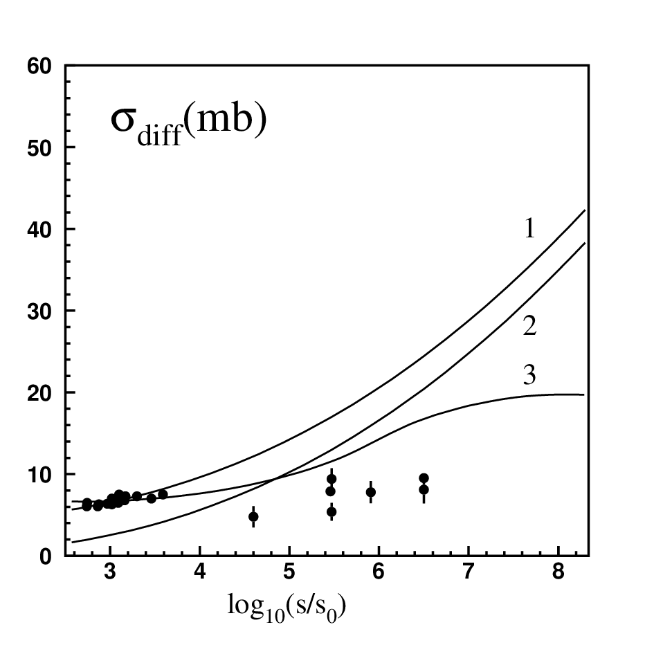


The results of our calculation show that in the large range of energies, the N=4 SYM scattering amplitude behaves as with a rather small coefficient in front. The graviton reggeization that will stop the anti-Froissart behavior at ultra high energies, does not show up at the accessible range of energy from the fixed target Fermilab energy, until the Tevatron energy. This reggeization can be measured, perhaps, only at the LHC energy.
4 Conclusion
In this paper we show that the N=4 SYM total cross section violates the Froissart theorem, and in the huge range of energy this cross section is proportional to . The graviton reggeization will change this increase to the normal logarithmic behavior . However, we demonstrated that this happens at ultra high energy, much higher than the LHC energy for reasonably low .
We need to assume that there is a different source for the total cross section, with the value of the cross section about 40 mb. With this assumption we successfully describe and for the accessible range of energy from the fixed target Fermilab to the Tevatron energies. The N=4 SYM mechanism is responsible only for a small part of the inelastic cross section for this energy region (about ). However, at the LHC energy the N=4 SYM theory can lead to a valuable contribution to the inelastic cross section, namely, which is about a quarter of the total inelastic cross section. The second surprise is the fact that the total cross section and the diffraction cross section can increase considerably from the Tevatron to the LHC energy. The bad description of gives the strong argument that the non N=4 SYM background should depend on energy.
It means that at RHIC energies, the N=4 SYM part of the inelastic cross section is negligible and the quark-gluon plasma is created by the mechanism outside of N=4 SYM. For the LHC energy, we can expect that N=4 SYM is responsible for the inelastic cross section of about out of .
We believe that we have a dilemma: to find a new mechanism for the inelastic production in the framework of N=4 SYM other than the reggeized graviton interaction, or to accept that N=4 SYM is irrelevant to description of any experimental data that have been measured before the LHC era, with a chance that even at the LHC it will be responsible only for a quarter (or less) of the total cross section. Deeply in our hearts, we believe in the first way out, and we hope that this paper will draw attention to this challenging problem: searching for a new mechanism for multiparticle production in N=4 SYM.
We wish to draw your attention to the fact that the scattering amplitude can change considerably from the Tevatron to LHC energy (see Table 1). Therefore, all claims that we can give reliable predictions for the values of the cross sections at the LHC energy and even of the survival probability for the diffractive Higgs production [27] looks exclusively naive and reflects our prejudice rather than our understanding.
Acknowledgments
We thank Boris Koppeliovich for fruitful discussion on the subject of the paper. Our special thanks go to Miguel Costa and Jeremy Miller for their careful reading of the first version of this paper and useful discussions. E.L. also thanks the high energy theory group of the University Federico Santa Maria for the hospitality and creative atmosphere during his visit.
This work was supported in part by Fondecyt (Chile) grants, numbers 1050589, 7080067 and 7080071, by DFG (Germany) grant PI182/3-1 and by BSF grant 20004019.
References
- [1] J. M. Maldacena, Adv. Theor. Math. Phys. 2 (1998) 231 [Int. J. Theor. Phys. 38 (1999) 1113] [arXiv:hep-th/9711200]; S. S. Gubser, I. R. Klebanov and A. M. Polyakov, Phys. Lett. B 428 (1998) 105 [arXiv:hep-th/9802109]; E. Witten, Adv. Theor. Math. Phys. 2 (1998) 505 [arXiv:hep-th/9803131].
- [2] J. Polchinski and M. J. Strassler, JHEP 0305 (2003) 012 [arXiv:hep-th/0209211]; Phys. Rev. Lett. 88 (2002) 031601 [arXiv:hep-th/0109174].
- [3] A. V. Kotikov, L. N. Lipatov, A. I. Onishchenko and V. N. Velizhanin, Phys. Lett. B 595 (2004) 521 [Erratum-ibid. B 632 (2006) 754] [arXiv:hep-th/0404092]; A. V. Kotikov and L. N. Lipatov, Nucl. Phys. B 661 (2003) 19 [Erratum-ibid. B 685 (2004) 405] [arXiv:hep-ph/0208220]; A. V. Kotikov and L. N. Lipatov, Nucl. Phys. B 582 (2000) 19 [arXiv:hep-ph/0004008]. A. V. Kotikov, L. N. Lipatov and V. N. Velizhanin, Phys. Lett. B 557 (2003) 114 [arXiv:hep-ph/0301021]; J. R. Andersen and A. Sabio Vera, Nucl. Phys. B 699 (2004) 90 [arXiv:hep-th/0406009]; Z. Bern, M. Czakon, L. J. Dixon, D. A. Kosower and V. A. Smirnov, Phys. Rev. D 75 (2007) 085010 [arXiv:hep-th/0610248]; Z. Bern, L. J. Dixon and V. A. Smirnov, Phys. Rev. D 72 (2005) 085001 [arXiv:hep-th/0505205];
- [4] Y. Hatta, E. Iancu and A. H. Mueller, JHEP 0801 (2008) 026 [arXiv:0710.2148 [hep-th]].
- [5] R. C. Brower, J. Polchinski, M. J. Strassler and C. I. Tan, JHEP 0712 (2007) 005 [arXiv:hep-th/0603115].
- [6] R. C. Brower, M. J. Strassler and C. I. Tan, arXiv:0707.2408 [hep-th].
- [7] R. C. Brower, M. J. Strassler and C. I. Tan, JHEP 0806 (2008) 048 [arXiv:0801.3002 [hep-th]].
- [8] L. Cornalba and M. S. Costa, Phys. Rev. D 78, (2008) 09010, arXiv:0804.1562 [hep-ph]; L. Cornalba, M. S. Costa and J. Penedones, JHEP 0806 (2008) 048 [arXiv:0801.3002 [hep-th]]; JHEP 0709 (2007) 037 [arXiv:0707.0120 [hep-th]].
- [9] B. Pire, C. Roiesnel, L. Szymanowski and S. Wallon, Phys. Lett. B 670, 84 (2008) [arXiv:0805.4346 [hep-ph]].
- [10] E. Levin, J. Miller, B. Z. Kopeliovich and I. Schmidt, JHEP 0902 (2009) 048; arXiv:0811.3586 [hep-ph].
- [11] L. V. Gribov, E. M. Levin and M. G. Ryskin, Phys. Rep. 100, 1 (1983).
- [12] A. H. Mueller and J. Qiu, Nucl. Phys. B 268 427 (1986) .
- [13] L. McLerran and R. Venugopalan, Phys. Rev. D 49,2233, 3352 (1994); D 50,2225 (1994); D 53,458 (1996); D 59,09400 (1999).
- [14] E. A. Kuraev, L. N. Lipatov, and F. S. Fadin, Sov. Phys. JETP 45, 199 (1977); Ya. Ya. Balitsky and L. N. Lipatov, Sov. J. Nucl. Phys. 28, 22 (1978).
- [15] I. Balitsky, [arXiv:hep-ph/9509348]; Phys. Rev. D60, 014020 (1999) [arXiv:hep-ph/9812311] Y. V. Kovchegov, Phys. Rev. D60, 034008 (1999), [arXiv:hep-ph/9901281].
- [16] J. Jalilian-Marian, A. Kovner, A. Leonidov and H. Weigert, Phys. Rev. D59, 014014 (1999), [arXiv:hep-ph/9706377]; Nucl. Phys. B504, 415 (1997), [arXiv:hep-ph/9701284]; J. Jalilian-Marian, A. Kovner and H. Weigert, Phys. Rev. D59, 014015 (1999), [arXiv:hep-ph/9709432]; A. Kovner, J. G. Milhano and H. Weigert, Phys. Rev. D62, 114005 (2000), [arXiv:hep-ph/0004014] ; E. Iancu, A. Leonidov and L. D. McLerran, Phys. Lett. B510, 133 (2001); [arXiv:hep-ph/0102009]; Nucl. Phys. A692, 583 (2001), [arXiv:hep-ph/0011241]; E. Ferreiro, E. Iancu, A. Leonidov and L. McLerran, Nucl. Phys. A703, 489 (2002), [arXiv:hep-ph/0109115]; H. Weigert, Nucl. Phys. A703, 823 (2002), [arXiv:hep-ph/0004044].
- [17] P. Kovtun, D. T. Son and A. O. Starinets, Phys. Rev. Lett. 94 (2005) 111601 [arXiv:hep-th/0405231].
- [18] C. P. Herzog, A. Karch, P. Kovtun, C. Kozcaz and L. G. Yaffe, JHEP 0607 (2006) 013 [arXiv:hep-th/0605158].
- [19] A. H. Mueller, Phys. Lett. B 668 (2008) 11 [arXiv:0805.3140 [hep-ph]]; F. Dominguez, C. Marquet, A. H. Mueller, B. Wu and B. W. Xiao, Nucl. Phys. A 811 (2008) 197 [arXiv:0803.3234 [nucl-th]]; Y. Hatta, E. Iancu and A. H. Mueller, JHEP 0805 (2008) 037 [arXiv:0803.2481 [hep-th]]
- [20] P. M. Chesler and L. G. Yaffe, Phys. Rev. D 78 (2008) 045013 [arXiv:0712.0050 [hep-th]]; A. Yarom, Phys. Rev. D 75 (2007) 105023 [arXiv:hep-th/0703095].
- [21] E. Witten, Adv. Theor. Math. Phys. 2 (1998) 253 [arXiv:hep-th/9802150].
- [22] I. Gradstein and I. Ryzhik, “ Tables of Series, Products, and Integrals”, Verlag MIR, Moskau,1981
- [23]
M. Froissart,
Phys. Rev. 123 (1961) 1053;
A. Martin, “Scattering Theory: Unitarity, Analitysity and Crossing.” Lecture Notes in Physics, Springer-Verlag, Berlin-Heidelberg-New-York, 1969. - [24] J. Naf, P. Jetzer and M. Sereno, Phys. Rev. D 79 (2009) 024014 [arXiv:0810.5426 [astro-ph]] ; L. Liu, arXiv:gr-qc/0411122 ;M. Novello and R. P. Neves, Class. Quantum Grav. 20 (2003) 67, arXiv:gr-qc/0210058.
- [25] E. D’Hoker, D. Z. Freedman, S. D. Mathur, A. Matusis and L. Rastelli, Nucl. Phys. B 562 (1999) 330 [arXiv:hep-th/9902042]; E. D’Hoker and D. Z. Freedman, Nucl. Phys. B 550 (1999) 261 [arXiv:hep-th/9811257]; D. Z. Freedman, S. D. Mathur, A. Matusis and L. Rastelli, Nucl. Phys. B 546 (1999) 96 [arXiv:hep-th/9804058]; E. D’Hoker, D. Z. Freedman, S. D. Mathur, A. Matusis and L. Rastelli, Nucl. Phys. B 562 (1999) 353 [arXiv:hep-th/9903196]; H. Liu, Phys. Rev. D 60 (1999) 106005 [arXiv:hep-th/9811152].
- [26] E. Gotsman, E. Levin, U. Maor and J. S. Miller, Eur. Phys. J. C 57 (2008) 689 [arXiv:0805.2799 [hep-ph]].
- [27] M. G. Ryskin, A. D. Martin and V. A. Khoze, Eur. Phys. J. C54 (2008) 199 [arXiv:0710.2494 [hep-ph]].