Gravitational-wave extraction from neutron-star oscillations
Abstract
We compare different gravitational-wave extraction methods used in three-dimensional nonlinear simulations against linear simulations of perturbations of spherical spacetimes with matter. We present results from fully general-relativistic simulations of a system composed by an oscillating and non-rotating star emitting gravitational radiation. Results about the onset of non-linear effects are also shown.
1 Simulation setup and wave extraction
We considered a stable equilibrium star model perturbed with an axisymmetric quadrupolar fluid perturbation. Assuming the perfect fluid approximation for the matter, the star is described by a polytropic equation of state of the type11 1 We use standard dimensionless units unless otherwise specified, for clarity. with , and central rest-mass density . The gravitational mass and the radius are and . This model has been widely used in the literature (see e.g. [10]). The perturbation consists in an axisymmetric pressure perturbation: the angular pattern is proportional to the spherical harmonic, while the radial profile has no nodes in the star interior. Different perturbation amplitudes are considered: , named ,, . After imposing the fluid perturbation, the linearized (Hamiltonian) constraint is solved under the hypothesis of conformal flatness to obtain consistently the perturbed metric. See [1, 3] for a detailed description and discussion.
The same initial data were then evolved with two different codes. The PerBaCCo code, described in [3], was used to solve in the time domain the (1+1) equations for the linear (even parity) perturbations of a spherical spacetime with matter. The resolution of the (radial) 1D grid is , which corresponds to points inside the star. Gravitational waves (GWs) are directly computed via the Zerilli-Moncrief function (see below). The Cactus-Carpet-CCATIE-Whisky code was instead used to solve the complete three-dimensional (3D) nonlinear hydrodynamics equations coupled with Einstein’s field equations within in the “3+1” formalism. See [2] for a general description of the code and the recent results obtained. The Cartesian 3D grid consists in 3 fixed refinement levels (boxes) with spacing (in each direction) or or for three resolutions used.
The extraction of gravitational radiation from a numerically computed spacetime is a non-trivial task . The current state-of-the-art methods employed by the numerical-relativity community are the metric extraction á la Abrahams-Price [4] and the curvature Newman-Penrose extraction via the Weyl scalar [5]. If are the multipoles of the GW degrees of freedom, the metric extraction provides the Zerilli-Moncrief and the Regge-Wheeler functions which are directly related to :
| (1) |
where . On the other hand if the curvature extraction is used, the GW multipoles must be recovered from the Weyl scalar using the relation
| (2) |
Because of the finite size of the numerical grid, GWs wave are extracted at finite radius.
In the following we analyze the performances of these methods in the “simple” system composed by a single oscillating star. All the results are compared with the 1D code which gives more accurate data for the waves. Our work, while differing from both, is motivated by the same ideas of [7, 6], namely testing the GW extraction methods with perturbative results and using an oscillating neutron star as a test-bed. It represents the first complete analysis of such a kind employing simulations with the Whisky code.
2 1D waveforms: wave identikit


We give here a detailed “identikit” of the waves emitted by the system considered and computed using the 1D perturbative simulations. This waves will serve as a starting point to compare with nonlinear simulations described in the following sections.
The data we are presenting came from a very long simulation with final time of about s. The full waveform is plotted in the top panel of Fig. 1. It can be described by two different phases: (i) an initial transient, of about half a GW cycle, say up to ms, related to the setup of the initial data (see the black solid line in the left-middle panel), followed by (ii) a quasi-harmonic oscillatory phase, where the matter dynamics are reflected into the stellar quasi-normal modes (QNMs):
| (3) |
From the Fourier spectrum of over a time interval from to about ms (see left-bottom panel), we found that the signal is dominated by the fundamental mode of oscillation of the star, the -mode, at frequency Hz, with a very weak contribution of the first pressure or -mode (at frequency around Hz). The accuracy of these frequencies obtained from Fourier analysis on such long time series has been checked in Ref. [3] and is better than 1%. The frequency of the -mode agrees with that of Ref. [10] within %. On the interval considered the waves can be perfectly represented by a one-mode expansion, i.e. Eq. 3 with . As a result of a standard least-squares nonlinear fit with a one-mode template we obtained the frequency Hz, which is perfectly consistent with that obtained via Fourier analysis. For the damping time, we estimated and thus s. The global residual ( norm) of the fit is of the order of .
If we consider the entire duration (1 s) of the signal it is clear that a one-mode expansion is not sufficient to reproduce accurately the waveform (see Figure 1). The Fourier analysis of the whole waveform reveals the presence of the -mode, which has longer damping time, and the entire signal has been fitted with a two-mode QNM expansion. The estimated values for the frequency of the -mode and the -mode are and , respectively, and the corresponding dumping times s and s, with errors respectively of the order of % and %. The frequencies are consistent with those computed via Fourier analysis as well as via the dumping times. This result is particularly significant for a time-domain code.
Figure 1 shows the extraction result at (isotropic) radius of , which is the same extraction radius used for the comparison with the 3D results. However in the 1D simulations we can easily reach up to . We checked (see Figure 2) the convergence of the waves with the extraction radius using as a reference point the maximum of . This point can be accurately fitted, as a function of the extraction radius, with
| (4) |
The extrapolated quantity allows an estimate of the error related to the extraction at finite distance. The difference in amplitude of a wave extracted at with respect to a wave extracted at infinity is less than and frequency seems not to be affected (within our accuracy) by finite extraction effects.
3 3D waveforms: comparison in the linear regime


We focus first on the data relative to the smallest initial perturbation amplitude . The 3D simulations were performed for a simulation time of about 20 ms. Figure 3 summaries the results of our findings. The black solid line is the waveform computed with the perturbative code and presented in the previous section. We assume it to be the exact one. The waveform extracted from the 3D simulation with the Abrahams-Price method is the blue dashed line in the figure. The only difference with the perturbative result is the presence of a “burst” of radiation at the early times (see left panel) ms. In [1] we discussed in detail this feature of the metric wave extraction. The main conclusions are the following. (i) It is unphysical: it linearly grows with the extraction radius and produces a violation of the linearized Hamiltonian constraint at the wave-extraction level. (ii) It is related to an inaccurate implementation of the Zerilli-Moncrief function in the 3D code and it can be reproduced in the perturbative code introducing “by hand” inaccuracies (very low resolution, low-order approximations for finite differences). (iii) It is absent in vacuum simulations, e.g. binary black holes, where higher grid resolutions can be used. Apart from the junk the metric waveform is perfectly superposed (until ms) to the exact one; frequency and amplitude are consistent within the error bars.
The GWs extracted via the scalar require the solution of Eq. 2 to obtain the GW multipole (or equivalently the Zerilli-Moncrief function). The procedure we followed is described in Ref. [11] and consists in computing a double integral of (the “bare” metric waveform) and then correcting it by subtracting a polynomial floor. The red dashed-dotted line in Fig. 3 is the “bare” waveform: as suggested by the figure, and differently from Ref. [11], we found that a quadratic polynomial is here necessary to align the waveform (see the green dashed-dotted line). Once this tuning has been done the waveform is exactly superposed to the perturbative one and, differently from the metric waveform, it is free from the unphysical burst of junk radiation.
In summary we can conclude that, in the linear regime, both extraction methods give a very good agreement with the “exact” waveform but neither is free from drawbacks. On one hand the metric extraction contains a burst of junk radiation at early times that can compromise the study of phenomena in the first 5 ms of simulation (e.g. the neutron-star collapse to black hole or neutron-star -modes). On the other hand the curvature extraction requires tuning of the integration constants.
4 3D waveforms: the nonlinear regime
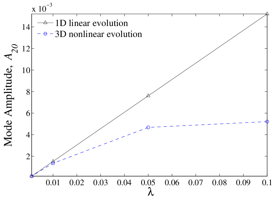

Finally we discuss nonlinear effects in the 3D waveforms. Previous studies can be found for example in [9] (second-order perturbation theory) and in [8] (CFC approximation of Einstein equations). We confirm those results without using approximations. Referring to the left panel of Fig. 4, we found that the amplitude of the mode (computed fitting Eq. 3) scales linearly with the initial perturbation amplitude - as expected -, but it progressively decreases in the nonlinear case due to excitation of other channels. The nonlinear effects are already visible for (10% difference in ) and quickly increase for (38%) and (66%). We note that the frequency of the wave, instead, is essentially not affected by nonlinearities with our setting.
Furthermore we considered the Fourier transform of the rest-mass density projected (multiplied and integrated on the 3D-space) on the spherical harmonic . As the right panel of Fig. 4 shows, for (green line) only the and (and ) mode frequencies are present, while for higher values of the spectra are rich of other frequencies. Most of the frequencies can be associated to the radial () fundamental frequency (1466 Hz), its overtone (5955 Hz), and to combination tones between the radial and the frequencies: . This analysis prove that mode couplings are present in the dynamics of the system already for small initial perturbation amplitudes, but they affect strongly only the amplitude of the GWs.
Acknowledgments
Computations have been performed on the INFN Beowulf clusters Albert at the University of Parma and on the Peyote and Damiana clusters at the Albert-Einstein-Institut.
References
- [1] L. Baiotti, S. Bernuzzi, G. Corvino, R. De Pietri and A. Nagar, Phys. Rev. D 79 (2009) 024002 [arXiv:0808.4002 [gr-qc]].
- [2] L. Baiotti, B. Giacomazzo and L. Rezzolla, Phys. Rev. D 78 (2008) 084033 [arXiv:0804.0594 [gr-qc]].
- [3] S. Bernuzzi and A. Nagar, Phys. Rev. D 78 (2008) 024024 [arXiv:0803.3804 [gr-qc]].
- [4] A. M. Abrahams and R. H. Price, Phys. Rev. D 53 (1996) 1963 [arXiv:gr-qc/9508059].
- [5] E. Newman and R. Penrose, J. Math. Phys. 3 (1962) 566.
- [6] M. Shibata and Y. I. Sekiguchi, Phys. Rev. D 68 (2003) 104020 [arXiv:astro-ph/0402184].
- [7] E. Pazos, E. N. Dorband, A. Nagar, C. Palenzuela, E. Schnetter and M. Tiglio, Class. Quant. Grav. 24 (2007) S341 [arXiv:gr-qc/0612149].
- [8] H. Dimmelmeier, J. A. Font and E. Muller, Astron. Astrophys. 393 (2002) 523 [arXiv:astro-ph/0204289].
- [9] A. Passamonti, N. Stergioulas and A. Nagar, Phys. Rev. D 75 (2007) 084038 [arXiv:gr-qc/0702099].
- [10] J. A. Font et al., Phys. Rev. D 65 (2002) 084024 [arXiv:gr-qc/0110047].
- [11] T. Damour, A. Nagar, M. Hannam, S. Husa and B. Bruegmann, Phys. Rev. D 78 (2008) 044039 [arXiv:0803.3162 [gr-qc]].