Emergence of Topological Fermi Liquid from a Strongly Correlated Bosonic System in Optical Superlattices

At unit-filling, the bosonic $t$-$J$ model is simple and can be reduced to AF Heisenberg model, $\hat{H}=J\sum_{\langle ij\rangle}\mathbf{\hat{S}}_{i}\cdot\mathbf{\hat{S}}_{j}$. A variational wave-function based on Resonating Valence Bond (RVB) picture by using Schwinger-boson description can produce[17, 18, 19] an unrivaled accurate ground-state energy; a generalized version[18] can further provide the staggered magnetization and spin excitation spectrum precisely. So the bosonic RVB picture is a natural choice for describing AF Heisenberg model. Explicitly, we can introduced two flavors of bosons on each site, created by a canonical operator $\hat{b}_{i\sigma}^{\dagger}$ acting on the vacuum $\left|0\right\rangle$ without bosons, satisfying $\hat{b}_{i\sigma}^{\dagger}\hat{b}_{i\sigma}=1$. This representation is equivalent to the following operator identity between the spin and boson operators $\mathbf{\hat{S}}_{i}=\frac{1}{2}\mathbf{\hat{b}}_{i}^{\dagger}\mathbf{\sigma\hat{b}}_{i}$. Here $\mathbf{\hat{b}}_{i}=(\hat{b}_{i\uparrow},\hat{b}_{i\downarrow})^{T}$ is a bosonic spinon annihilation operator. The mean-field value is characterized by a bosonic RVB order parameter $\Delta_{ij}^{s}=\langle\hat{b}_{i\sigma}\hat{b}_{j,-\sigma}\rangle\neq 0$ for the nearest-neighbor sites, which depicts the short-range AF correlation as $\langle\mathbf{\hat{S}}_{i}\cdot\mathbf{\hat{S}}_{j}\rangle=-\frac{1}{2}|\Delta_{ij}^{s}|^{2}$. At zero temperature, spinon $\mathbf{\hat{b}}$ becomes massless and Bose-condensation takes place with $\langle\mathbf{\hat{b}}\rangle\neq 0$, corresponding to the long-range Néel order in $x$-$y$ plane.

To learn the property of an AF order with vacancies, we should generalize the idea of spin-charge separation, which has become a very basic concept in understanding the doped Mott insulator related to high-$T_{c}$ cuprate[10, 20]. Unlike a usual quasi-particle that carries both spin and charge quantum numbers in conventional metals, it states that the system has two independent elementary excitations, the neutral spinon and the spinless holon. It is assumed that usual quasi-particle excitations may no longer be stable against the spin-charge separation mechanism once being created, e.g., by injecting a bare vacancy into the system; and it has to decay into more elementary spinons and holons. In other words, to theoretically describe the introduction of a single vacancy, one has to first annihilate a particle state $\left|\Psi\right\rangle$ together with a bosonic spinon $\hat{b}_{i\sigma}$, then generate a spinless operator $\hat{h}_{i}^{\dagger}$ denotes a holon (a vacancy) as

In addition, $\hat{h}_{i}^{\dagger}$ and $\hat{b}_{i\sigma}$ should satisfy the no-double-occupancy constraint, $\hat{h}_{i}^{\dagger}\hat{h}_{i}+\sum_{\sigma}\hat{b}_{i\sigma}^{\dagger}\hat{b}_{i\sigma}=1$. In contract to the case of high-$T_{c}$ cuprates, holons in bosonic $t$-$J$ model are neutral for they are actually the absence of cold atoms in a certain site.

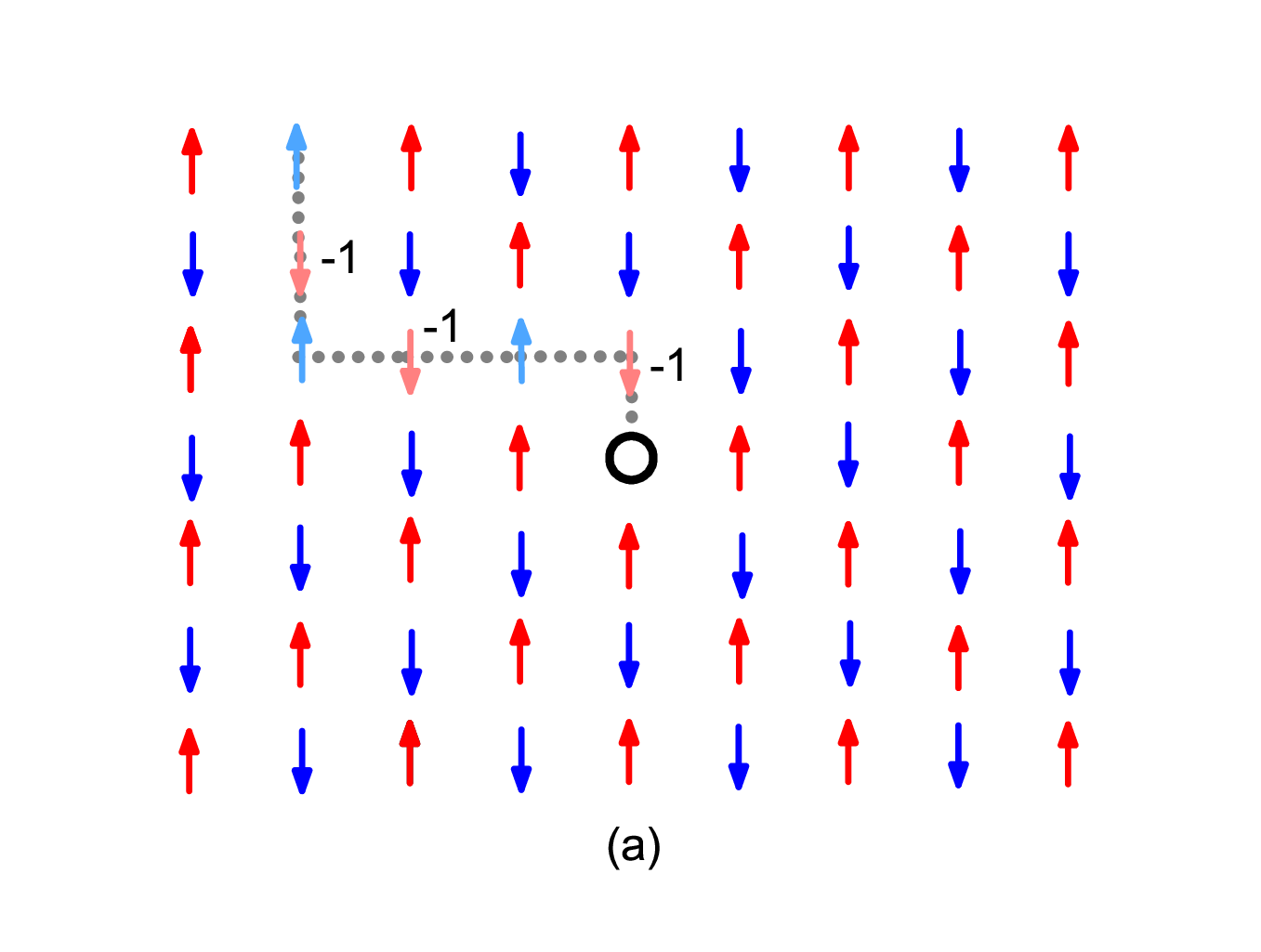
However, the situation changes when the hole moves. According to Marshall[21], the ground-state wave function of the Heisenberg Hamiltonian for a bipartite lattice satisfies a sign rule. It requires that flips of two antiparallel spins at nearest-neighbor sites are always accompanied by a sign change in the wave function: $\left|\cdots\uparrow\downarrow\cdots\right\rangle\mapsto\left(-1\right)\times\left|\cdots\downarrow\uparrow\cdots\right\rangle$. To show the sign effect in detail, we divide a bipartite lattice into odd ($A$) and even ($B$) sublattices and assign an extra sign $\left(-1\right)$ to every down spin at $A$ site. When the hole initially locating at site $i$ hops onto a nearest-neighbor site $j$, the Marshall sign rule is violated, resulting in a string of mismatched signs on the vacancy’s course[22]. The spin wave function is changed into

where $\hat{n}_{i\in A,\downarrow}^{b}=\hat{b}_{i\in A,\downarrow}^{\dagger}\hat{b}_{i\in A,\downarrow}$ is the number of down spin on each $A$-sublattice. In particular, if the hole moves through a closed path $C$ on the lattice to return to its original position, it will get a Berry phase $(-1)^{N_{C}^{\downarrow}}$, where $N_{C}^{\downarrow}$ is the total number of down spins “encountered” by the hole on the closed path $C$.[23, 24, 25] This process is illustrated in Fig. (2a).

To deal with this unavoidable Berry phase $(-1)^{N_{C}^{\downarrow}}$ in the ground-state wave function when there is mobile hole, we introduce a phase-string transformation[23] $|\tilde{\Psi}\rangle\mapsto e^{i\hat{\Theta}}|\tilde{\Psi}\rangle=|\Psi\rangle$, where $\hat{\Theta}=\sum_{ij}\theta_{ij}\hat{n}_{i}^{h}\hat{n}_{j\downarrow}^{b}$, $\hat{n}_{i}^{h}$ and $\hat{n}_{j\downarrow}^{b}$ are occupation number operators of the hole and down-spins, with a phase factor $\theta_{ij}=$Im$[\ln(z_{i}-z_{j})]$. Here $z\equiv x+iy$ denotes position and the subscripts $i$ and $j$ denote lattice sites. Considering the single-occupancy constraint, $\hat{\Theta}=-\frac{1}{2}\sum_{ij}\hat{n}_{i}^{h}\theta_{ij}[1-\hat{n}_{j}^{h}-\sum_{\sigma}\left(-1\right)^{\sigma}\hat{n}_{j\sigma}^{b}]$, where $\left(-1\right)^{\uparrow}\equiv 1$, $\left(-1\right)^{\downarrow}\equiv-1$. The phase-shift factor $e^{i\hat{\Theta}}$ can also be regarded as a unitary transformation on an arbitrary operator: $\hat{O}\mapsto e^{i\hat{\Theta}}\hat{O}e^{-i{\hat{\Theta}}}$. For example, operators of holons $\hat{h}_{i}^{\dagger}$ and spinons $\hat{b}_{i\sigma}$ are transformed as follow,

Now we have restored the simple spin wave function $|\Psi\rangle$ as equation (2) originally defined, but have got a set of nontrivial operators, and it is just the aim of the above transformation.

Furthermore, by defining $\hat{h}_{i}^{\prime\dagger}=\hat{h}_{i}^{\dagger}e^{-i\sum_{j}\theta_{ij}\hat{n}_{j}^{h}}$, we can see that except for a phase factor $e^{\frac{i}{2}\sum_{j}\theta_{ij}}$, holon $\hat{h}_{i}$ and spinon $\hat{b}_{i\sigma}$ are symmetric,

namely, $\hat{h}_{i}\overset{h\rightarrow b,\ i\rightarrow i\sigma}{\longmapsto}\hat{b}_{i\sigma}$ and $\hat{b}_{i\sigma}\overset{b\rightarrow h,\ i\sigma\rightarrow i}{\longmapsto}\hat{h}_{i}.$ The phase factor $e^{\frac{i}{2}\sum_{j}\theta_{ij}}$ means an additional lattice $\pi$-flux-per-plaquette for holons. From equation (3), one can see that there exists a mutual semionic statistics between holons and spinons, where holons perceive spinons as $\pi$-vortices and vice versa. In particular, after the transformation $\hat{h}_{i}^{\prime\dagger}=\hat{h}_{i}^{\dagger}e^{-i\sum_{j}\theta_{ij}\hat{n}_{j}^{h}}$, $\hat{h}_{i}^{\prime\dagger}$ obeys fermionic anti-commutation[26],

Finally, based on the RVB ground state by considering the phase string effect[23, 24, 25], the effective Hamiltonian of holons in bosonic $t$-$J$ model can be written as

where $t_{h}\approx|\Delta_{ij}^{s}|t$ is the effective hopping amplitude of holons, $\mu$ is the chemical potential. The gauge field $\hat{a}_{ij}$ satisfy the topological constraint $\sum_{C}\hat{a}_{ij}=\pm\pi\sum_{l\in C}(\hat{n}_{l\uparrow}^{b}-\hat{n}_{l\downarrow}^{b})$ for a closed loop $C$, $\phi_{ij}^{0}$ describes a $\pi$ flux per plaquette, $\sum_{\square}\phi_{ij}^{0}=\pm\pi$. It is obvious that the difference between fermionic $t$-$J$ model and bosonic $t$-$J$ model is the statistic of holons: in former case, holons are bosons; and in latter case, they are fermions.

Now we may be able to answer the question: what is the fate of a holon in an AF order? As we have mentioned above, the AF order lying in $x$-$y$ plane can be seen as a Bose condensation of spinons, $\langle\hat{b}_{i\sigma}\rangle\neq 0$. According to the above effective Hamiltonian (4), and the quantity $\hat{S}_{i}^{\dagger}=(-1)^{i}\hat{b}_{i\uparrow}^{\dagger}\hat{b}_{i\downarrow}e^{i\sum_{j}\theta_{ij}\hat{n}_{j}^{h}}$, a holon introduced here is a topological defect carrying spin twists and changing its peripheral spin configuration, as a meron-like object[27, 28, 29, 30], such a spin vortex (for a holon at the origin) may be characterized by a unit vector $\mathbf{n}_{i}=\mathbf{(-}1\mathbf{)}^{i}\left\langle\mathbf{S}_{i}\right\rangle/S$,

This meron-like spin configuration is schematically shown in Fig. (2b).

By now, one may imagine that a single hole would become a meron in a long-range AF order. However, the answer is not quite right. For a single meron configuration, the energy is logarithmically divergent, $E\approx J|\Delta_{ij}^{s}|\mathrm{\ln}\left(L/a_{0}\right)$ with $L$ the size of the system. In order to remove this infinite-energy cost, as in the present case, each holon-meron has to “nucleate” an anti-meron from the background spontaneously. Define $n_{i}^{x}+in_{i}^{y}=e^{i\phi_{0}+i\phi_{i}}$, with the unit vector $\mathbf{n}_{0}\equiv(\cos\phi_{0},\sin\phi_{0})$ as the magnetization direction at infinity. In presence of a fermionic holon centered at $-z_{k}/2$ and an anti-meron centered at $z_{k}/2$, we have[31, 32] $\phi_{i}^{k}=\mathrm{Im}\ln\left[\left(z_{i}-z_{k}/2\right)/\left(z_{i}+z_{k}/2\right)\right]$ with $z_{k}\equiv e_{k}^{x}+ie_{k}^{y}$. By using $\mathbf{\hat{e}}_{k}=(e_{k}^{x},e_{k}^{y})$ to denote the spatial displacement of the holon and anti-meron centered, a dipolar spin configuration at a sufficiently large distance is obtained,

Thus, each pair of holons and anti-merons forms a composite, as shown in Fig. (2c). In contrast to the logarithmically divergent meron-energy, the energy a dipole $E_{d}$ becomes finite[31, 32], $E_{d}\approx J|\Delta_{ij}^{s}|\ln\left[\left(\left|\mathbf{\hat{e}}_{k}\right|+a_{0}\right)/a_{0}\right]$, $\left|\mathbf{\hat{e}}_{k}\right|\gtrsim a_{0}$.

Physically, one may consider a bare hole (spinless holon) created by an annihilation operator $\hat{h}^{\dagger}$ at point $a$, then it may jump to point $b$ via some discrete steps, being connected by a phase string in between. Since the holon can reach $b$ through different virtual paths originated at $a$, this singular phase string is then replaced by, or relaxes to, a smooth dipole configuration. An anti-meron itself is a semi-vortex formed by condensed spinons and it is immobile. Therefore, the hole-dipole as a whole must remain localized (self-trapped) in space. The resulting spin configuration has a dipolar symmetry while the distortion of the direction of magnetization is long ranged and decays as $r^{-1}$[32, 33].

In the lightly doped region, $\delta\rightarrow 0$, there exist localized holes that are self-trapped around anti-merons via a logarithmically confining potential $V\left(r\right)\approx q^{2}\ln\left(\left|\mathbf{r}\right|/a\right)$, $q^{2}=2\pi J|\Delta_{ij}^{s}|$, and their dipolar moments are randomly distributed. Such kind of AF ordered state with random dipoles has been studied in refs. [36, 37, 38, 31]. It is known that when $T=0$, the spin-correlation length is finite for arbitrary doping $\delta$. This implies the destruction of long-range AF order, as long as $\delta>0$. Consequently, AF order is limited mainly in finite sizes, where the size $\xi$ of a domain is determined by the hole’s concentration, $\xi\approx a/\sqrt{\delta}$. Accordingly, this state has been termed as a cluster spin glass[39, 40]. The spin glass freezing temperature is then expected to vary as $T_{g}\varpropto\xi^{2}\varpropto a^{2}/\delta$, below which holons tend to form a glass and their dynamics strongly slows down.

When doping increases, more and more dipoles appear. As a result, the “confining” potential $V\left(r\right)$ between these dipoles will be screened by polarizations of pairs lying between them. When this screening effect becomes so strong that even the largest pair has to break up, holons and anti-merons are liberated to move individually. This qualitative analysis suggests that a localization-delocalization phase transition should occur at a critical point $\delta_{c}$, in a fashion of the Kosterlitz-Thouless (KT) transition. Using the renormalization group method[35, 31], one can determine the critical hole density $\delta_{c}=\delta_{c}(T)$ or temperature $T_{\mathrm{de}}=T_{\mathrm{de}}(\delta)$ at which dipoles collapse and holon-merons are “deconfined” from the bound state with anti-merons. At zero temperature, the critical hole density has been numerically determined as

Therefore, a zero-temperature quantum critical point exists at $\delta_{c}=0.043$ where hole-dipoles dissolve into holon-merons and anti-merons.

When $\delta>0.043$, fermionic holons are delocalized, so a Fermi surface emerges in the momentum space. And since two holons always repulse each other, for they are merons with same topological charges, then these fermions cannot pair with each other and it makes the Fermi surface stable. This is different from the case where electrons form Cooper pairs in superconductors, because here we have topological repulsions not electronic repulsions.

Thus, we display the global phase-diagram of bosonic $t$-$J$ model in Fig. (3). There exists three different regions globally: region I, AF insulator, $\delta=0$; region II, insulating spin-glass (SG), $\delta\in\left(0,0.043\right)$; region III, topological Fermi-liquid (TFL) phase with spin-liquid ground state, $\delta\in\left(0.043,0.5\right)$. The phase boundary that protects the physics in low doping regimes can be written as $k_{B}T\approx c\left(1-2\delta\right)J,\ c$ is an integration quantity (see Methods). Particularly, our results illustrate the emergence of an exotic fermionic state (TFL) in a pure bosonic system.

In TFL state, the effective Hamiltonian of holons can be written as

and the dispersion relation is

as Fig. (4) shows.

In Fig. (5), we show the evolution of Fermi surfaces by plotting four doping cases, $\delta=0.05$, $0.1$, $0.15$ and $0.2$, respectively. From the global phase diagram Fig. (3) and Fig. (5), we suggest that in experiments people may observe TFL in bosonic $t$-$J$ model of $15\%$ hole concentration, of which highest Fermi energy with clear Fermi surfaces are predicted.

Besides, when holon moves, the spin configuration changes simultaneously, thus there is no long-range AF order anymore. Instead, the magnetic ground-state becomes a spin liquid state with invariant spin-rotation and translation symmetry. Without anti-merons matching with holons, holons exert an “effective magnetic field” on spinons (recall the mutual relation between the two excitations), $B_{h}=\pi\rho_{h}$ with $\rho_{h}$ the density of holons. Hence, a new length scale is introduced to the spinon system, which is the magnetic cyclotron length $l_{c}=B_{h}^{-1/2}$. $l_{c}$ will later be connected to the remaining magnetic correlation length.

As we mentioned above, doping creates a Landau-level structure in the spinon spectrum. Thus, low-lying spin fluctuations are expected to be sensitive to dopants. After calculations, we find

Here $\chi^{\prime\prime}\left(\mathbf{q},\omega\right)$ is defined as ($\beta=1/k_{B}T$)

where $\left\langle\mathbf{S}\left(\mathbf{r},t\right)\cdot\mathbf{S}\left(0,0\right)\right\rangle$ is the spin-spin correlation function. This is a Gaussian type around the AF wave-vector $\mathbf{Q}_{0}=(\pm\pi,\pm\pi)/a_{0}$ with a width $l_{c}^{-1}$. Consequently, it determines the spin-spin correlation in the real space as $\cos\left(\mathbf{Q}_{0}\cdot\mathbf{r}\right)e^{-\left|\mathbf{r}\right|^{2}/\xi^{2}}$, where the correlation length $\xi=\sqrt{2}l_{c}=a_{0}\sqrt{2/\left(\pi\delta\right)}$ is in the same order of the average hole-hole distance[41]. Namely, doped holes break up the long-range AF correlation into short-range AF fragments within a length scale of $\xi$.

In contrast, the ground-state of fermionic $t$-$J$ model is a superconducting state of condensed holons, in which spin liquid state is always masked by holons’ condensation[42]. While in bosonic $t$-$J$ model, it is the topological Fermi liquid state with massless fermionic excitations, in which one can easily detect properties of this spin liquid state. For these reasons, the observation of this exotic quantum state (TFL with short range spin correlation) in bosonic $t$-$J$ model may pave an alternative approach to verify the microscopic theory of high $T_{c}$ superconductivity.

In region I and II, the system is an insulator in the first place, so the momentum distribution is universal and isotropic in the Brillouin zone (without considering the trapping and boundary conditions). This feature can be detected by measuring density profile measurement[44], or via Bragg spectroscopy[43] to observe the momentum spectrum. Additionally, in the Néel state (I), the condensate exhibits long range AF order, while in the spin glass state (II), this long ranged magnetic order disappears. This difference can be distinguished through spatial spin-spin correlations, $\langle\hat{S}_{z}\left(\mathbf{r}_{1}\right)\hat{S}_{z}\left(\mathbf{r}_{2}\right)\rangle$. As demonstrated in refs.[45, 46], using a probe laser beam which goes through the condensate, one can measure the phase shift or change of polarization of the outgoing beam $\langle\hat{X}_{\text{out}}\rangle$ to obtain the magnetization $\langle\hat{X}_{\text{out}}\rangle\propto\langle\hat{M}_{z}\rangle\propto\int d\mathbf{r}\phi\left(\mathbf{r}\right)\langle\hat{S}_{z}\left(\mathbf{r}\right)\rangle$, where $\phi\left(\mathbf{r}\right)$ is the spatial intensity profile of the laser beam. The quantum noise $\langle\hat{X}_{\text{out}}^{2}\rangle\propto\langle\hat{M}_{z}^{2}\rangle\propto\int d\mathbf{r}_{1}d\mathbf{r}_{2}\phi\left(\mathbf{r}_{1}\right)\phi\left(\mathbf{r}_{2}\right)\langle\hat{S}_{z}\left(\mathbf{r}_{1}\right)\rangle\langle\hat{S}_{z}\left(\mathbf{r}_{2}\right)\rangle$ reveals the atomic correlations in the system. This method can directly examine the existence of 2D AF correlations.

In region III, we have demonstrated that one natural characteristic of TFL is the existence of Fermi surfaces in the Brillouin zone. Esslinger et al.[47] had successfully observed the Fermi surface in a 3D optical lattice filled with fermionic atoms. Similarly, one may also observe these Fermi levels in our bosonic system, as shown in Fig. (5). Besides, the short-range AF fluctuations may also be observed. As equation (5) indicates, the spin dynamic structure factor as well as the dynamic spin susceptibility function are linked with spin-spin correlations. The latter one reflects the effective short-range magnetic correlation length $\xi$.

To sum up, in this paper, we first demonstrate the implementation of bosonic $t$-$J$ model in optical superlattices filled with a two-component BEC. And for the first time, we systematically discussed the possible quantum phases of this model upon doping. A key feature is the mutual semionic statistics between the two elementary excitations of the system, holons and spinons. When there are only a few holes around, they tend to form hole-dipoles, locally changing the underlying spin texture into meron-anti-meron pairs. At low doping, the deformed spin configuration loses the long-range order, and there emerges a spin glass state. When holes are prevailing, through a quantum phase transition ($\delta_{c}=0.043$) that frees those self-localized holons in spin glass state, a strange topological Fermi liquid with Fermi surface appears in a purely bosonic system, as a significant result of the mutual statistics between holons and spinons. We also list accessible experimental approaches to verify and detect these novel theoretical predictions.