1Introduction

HISKP–TH–08/23, FZJ-IKP-TH–2008–22

The mass of the $\Delta$ resonance in a finite volume:
fourth-order calculation

August 24, 2026

V. Bernard^a, D. Hoja^b, U.-G. Meißner^b,c and A. Rusetsky^b

{}^{a}\,

Groupe de Physique Theorique, IPN, CNRS/Université Paris Sud 11

F-91406 Orsay Cedex France

{}^{b}\,

Helmholtz–Institut für Strahlen– und Kernphysik and

Bethe Center for Theoretical Physics

Universität Bonn, D–53115 Bonn, Germany

^cInstitut für Kernphysik, Institute for Advanced Simulations

and Jülich Center for Hadron Physcis

Forschungszentrum Jülich, D-52425 Jülich, Germany

Pacs:	11.10.St, 11.15.Ha, 12.39.Fe
Keywords:	Resonances in lattice QCD, field theory in a finite volume,
	chiral perturbation theory, small scale expansion

Abstract

We calculate the self-energy of the $\Delta(1232)$ resonance in a finite volume, using chiral effective field theory with explicit spin-3/2 fields. The calculations are performed up-to-and-including fourth order in the small scale expansion and yield an explicit parameterization of the energy spectrum of the interacting pion-nucleon pair in a finite box in terms of both the quark mass and the box size $L$ . It is shown that finite-volume corrections can be sizeable at small quark masses.

1 Introduction

The recent surge of interest in lattice calculations of the excited baryon spectrum [1, 2, 3, 4, 5, 6, 7, 8, 9, 10, 11, 12, 13, 14, 15, 16, 17, 18, 19] has been mainly motivated by the experimental resonance physics program at Jefferson Lab [20] and ELSA [21]. Also, the hadron spectrum is arguably the least understood feature of Quantum Chromodynamics. In general, the extraction of the properties of the excited states from the lattice data is a more delicate enterprise as compared to the ground-state hadrons. The reason is that the excited states are unstable and, strictly speaking, can not be put in correspondence to a single isolated level in the discrete spectrum measured in lattice simulations. A standard procedure proposed by Lüscher [22, 23, 24, 25] (see also [26, 27, 28, 29, 30]) consists in placing the system into a finite cubic box of a size $L$ and studying the response of the spectrum on the change of $L$ . It can be shown that the dependence of the energy levels on $L$ is dictated solely by the scattering phase shift in the infinite volume. Consequently, the method is capable of extracting the phase shift from the lattice data that also determines the position and the width of the resonances (see, e.g. [31, 32, 19]). Recently, the above approach has been also applied to study nucleon-nucleon phase shifts at low energy, as well as the two-body shallow bound states [33, 34, 35, 36, 37].

Alternative approaches to study the decaying states have been suggested, see, e.g. [38, 39, 40]. In particular, an interesting proposal is to reconstruct the spectral function by using the maximal entropy method [41], which can also be used to address the problem of unstable systems.

In actual calculations on the lattice the quark masses do not usually coincide with physical quark masses. This qualitatively changes the picture since, if the quark mass is large enough, the $\Delta(1232)$ does not decay and can be extracted by the methods applicable in case of the stable particles. Reducing the quark mass, a value is reached such that the $\Delta$ starts to decay into a pion and a nucleon^#1^#1 #1 The decay threshold is located at $M_{N}+M_{\pi}=M_{\Delta}$ in the infinite volume. In a finite volume, the decay of $\Delta$ at threshold in the center-of-mass (CM) frame is forbidden. Still, for brevity, the point $M_{N}+M_{\pi}=M_{\Delta}$ will be always referred below to as the threshold.. The spectrum becomes strongly volume-dependent and Lüscher’s method has to be applied to extract the parameters of the resonance – the mass and the width.

Above the threshold $M_{N}+M_{\pi}>M_{\Delta}$ , the finite-volume corrections to the spectrum are exponentially suppressed and can be neglected in the first approximation. However, for those values of the quark masses which correspond to $M_{N}+M_{\pi}<M_{\Delta}$ , finite-volume corrections may become large and should be taken into account. Note that merely making the volume larger does not suffice in the case of an unstable state. Due to the potentially large corrections, the finite volume data on the finite-volume energy spectrum can be enhanced below threshold. This enhancement, which is visible in the lattice data at smaller volumes, can not be described by using the formulae for the quark mass dependence in the infinite volume. We shall demonstrate an explicit example of such a behavior below.

From the above discussion it is clear that, in order to be able to include all available lattice data for large as well as small quark masses in the analysis, one needs to provide a simultaneous explicit parameterization of the lattice QCD spectrum in terms of both the quark mass $\hat{m}$ and the box size $L$ . This goal can be achieved by invoking the chiral effective field theory with explicit spin-3/2 degrees of freedom [42, 43] in a finite volume. The first attempt in this direction was made in Ref. [44], where we have performed the calculations of the finite-volume energy spectrum at third order in the so-called small scale expansion (SSE). The present paper extends these calculations to the fourth order. In addition,

i)

We provide an explicit formula for the finite-volume corrections for the unstable $\Delta$ , which can be used in the analysis of the lattice data;
ii)

We perform a fit of the obtained expressions to the most recent available data at different quark masses, taking into account finite-volume corrections. The fit allows one to determine some of the low-energy constants (LECs) in the chiral Lagrangian;
iii)

In doing so, one does not need to resort to any input phenomenological parameterization of the resonant amplitude, because SSE provides such a parameterization automatically, order by order in the $\epsilon$ -expansion (here, $\epsilon$ denotes the formal small expansion parameter in the SSE).
iv)

We analyze the quark mass dependence of the spectrum by using the method of probability distribution, introduced in [45].

Note also that in this paper we do not consider the finite-volume effects in the stable particle masses, which are exponentially suppressed at large volumes. Such effects can be treated within the same approach, see, e.g. Ref. [46].

The layout of the paper is as follows. In section 2 we discuss the calculation of the mass of the nucleon and the $\Delta$ in the infinite volume, at fourth order in the small scale expansion. In section 3 the calculation of the finite-volume energy spectrum of the $\pi N$ system is addressed. In section 4 we consider the fit of the explicit analytic expressions for the nucleon and $\Delta$ mass to the existing data from lattice QCD and determine some of the LECs of the chiral Lagrangian. We also analyze the finite volume spectrum with the use of probability distributions [45]. Finally, section 5 contains our conclusions.

2 The mass of the nucleon and the $\Delta$ resonance in the infinite volume

Our calculations will be carried out in two steps. We first perform calculations of the nucleon and $\Delta$ mass at order $\epsilon^{4}$ in the infinite volume^#2^#2 #2 The small parameter $\epsilon$ subsumes external momenta, the pion mass and the nucleon-delta mass splitting. . At the second step, we use the same Lagrangian in order to carry out the calculations of the finite-volume energy spectrum. The results of these calculations are applied to the case of an unstable $\Delta$ .

The Lagrangian of pions, nucleons and deltas up-to-and-including order $\epsilon^{4}$ in the SSE is taken from Ref. [47]. Below we display only those terms that contribute to the nucleon and $\Delta$ mass at this order,

{\cal L}=\sum\limits_{i=1}^{4}\left({\cal L}_{\pi N}^{(i)}+{\cal L}_{\pi\Delta}^{(i)}\right)+\sum\limits_{i=1}^{2}{\cal L}_{\pi N\Delta}^{(i)}\,,

(1)

where the pion–nucleon Lagrangians are given by

$\displaystyle{\cal L}_{\pi N}^{(1)}$	$\displaystyle=$	$\displaystyle\bar{\psi}_{N}\left[i\not{D}-\mathring{m}_{N}+\frac{g_{A}}{2}\,\not{u}\gamma_{5}\right]\psi_{N}\,,$
$\displaystyle{\cal L}_{\pi N}^{(2)}$	$\displaystyle=$	$\displaystyle\bar{\psi}_{N}\left[c_{1}\langle\chi_{+}\rangle-\frac{c_{2}}{4\mathring{m}_{N}^{2}}\,\left(\langle u_{\mu}u_{\nu}\rangle D^{\mu}D^{\nu}+\text{h.c.}\right)+\frac{c_{3}}{2}\,\langle u^{2}\rangle+\ldots\right]\psi_{N}\,,$
$\displaystyle{\cal L}_{\pi N}^{(3)}$	$\displaystyle=$	$\displaystyle\bar{\psi}_{N}\left[B_{23}\Delta_{0}\langle\chi_{+}\rangle+B_{32}\Delta_{0}^{3}+\ldots\right]\psi_{N}\,,$

	$\displaystyle{\cal L}_{\pi N}^{(4)}$	$\displaystyle=$	$\displaystyle\bar{\psi}_{N}\Bigl[e_{38}\langle\chi_{+}\rangle^{2}+\frac{1}{4}\,e_{115}\langle\chi_{+}^{2}-\chi_{-}^{2}\rangle-\frac{1}{4}\,e_{116}\left[\langle\chi_{-}^{2}\rangle-\langle\chi_{-}\rangle^{2}+\langle\chi_{+}^{2}\rangle-\langle\chi_{+}\rangle^{2}\right]$		(2)
		$\displaystyle+$	$\displaystyle E_{1}\Delta_{0}^{4}+E_{2}\Delta_{0}^{2}\langle\chi_{+}\rangle+\ldots\Bigr]\psi_{N}\,,$		(2)

and

$\displaystyle{\cal L}_{\pi\Delta}^{(1)}$	$\displaystyle=$	$\displaystyle-\bar{\psi}_{\alpha}^{i}O^{\alpha\mu}\Bigl\{\left[i\not{D}^{ij}-\mathring{m}_{\Delta}\xi_{3/2}^{ij}+\frac{g_{1}}{2}\,\not{u}^{ij}\gamma_{5}\right]g_{\mu\nu}-\frac{1}{4}\left[\gamma_{\mu}\gamma_{\nu}\,,\,\left(i\not{D}^{ij}-\mathring{m}_{\Delta}\xi_{3/2}^{ij}\right)\right]\Bigr\}\,O^{\nu\beta}\psi_{\beta}^{j}\,,$
$\displaystyle{\cal L}_{\pi\Delta}^{(2)}$	$\displaystyle=$	$\displaystyle-\bar{\psi}_{\alpha}^{i}O^{\alpha\mu}\Bigl\{\Bigl[a_{1}\langle\chi_{+}\rangle\delta^{ij}-\frac{a_{2}}{4\mathring{m}_{\Delta}^{2}}\,\left(\langle u_{\rho}u_{\sigma}\rangle D_{ik}^{\rho}D_{kj}^{\sigma}+\text{h.c.}\right)$
	$\displaystyle+$	$\displaystyle\frac{a_{3}}{2}\,\langle u^{2}\rangle\delta^{ij}+\ldots\Bigr]g_{\mu\nu}+\ldots\Bigr\}O^{\nu\beta}\psi_{\beta}^{j}\,,$
$\displaystyle{\cal L}_{\pi\Delta}^{(3)}$	$\displaystyle=$	$\displaystyle-\bar{\psi}_{\alpha}^{i}O^{\alpha\mu}\left[B_{1}^{\Delta}\Delta_{0}\langle\chi_{+}\rangle+B_{0}^{\Delta}\Delta_{0}^{3}+\ldots\right]g_{\mu\nu}\delta^{ij}O^{\nu\beta}\psi_{\beta}^{j}\,,$
$\displaystyle{\cal L}_{\pi\Delta}^{(4)}$	$\displaystyle=$	$\displaystyle-\bar{\psi}_{\alpha}^{i}O^{\alpha\mu}\Bigl[e_{38}^{\Delta}\langle\chi_{+}\rangle^{2}+\frac{1}{4}\,e_{115}^{\Delta}\langle\chi_{+}^{2}-\chi_{-}^{2}\rangle-\frac{1}{4}\,e_{116}^{\Delta}\left[\langle\chi_{-}^{2}\rangle-\langle\chi_{-}\rangle^{2}+\langle\chi_{+}^{2}\rangle-\langle\chi_{+}\rangle^{2}\right]$	(3)
	$\displaystyle+$	$\displaystyle E_{1}^{\Delta}\Delta_{0}^{4}+E_{2}^{\Delta}\Delta_{0}^{2}\langle\chi_{+}\rangle+\ldots\Bigr]g_{\mu\nu}\delta^{ij}O^{\nu\beta}\psi_{\beta}^{j}\,.$	(3)

The $\pi N\Delta$ interaction is described by the following Lagrangians

	$\displaystyle{\cal L}_{\pi N\Delta}^{(1)}$	$\displaystyle=$	$\displaystyle c_{A}\bar{\psi}_{\alpha}^{i}O^{\alpha\beta}w_{\beta}^{i}\psi_{N}\;+\;\text{h.c.}\,,$
	$\displaystyle{\cal L}_{\pi N\Delta}^{(2)}$	$\displaystyle=$	$\displaystyle\bar{\psi}_{\alpha}^{i}O^{\alpha\mu}\left[ib_{3}w_{\mu\nu}^{i}\gamma^{\nu}+i\frac{b_{6}}{\mathring{m}_{N}}\,w_{\mu\nu}^{i}iD^{\nu}+\ldots\right]\psi_{N}+\text{h.c.}\,.$		(4)

In the above expressions, $\psi_{N}$ and $\psi^{i}_{\mu}$ denote the nucleon and the $\Delta$ field, respectively, $\mathring{m}_{N}$ and $\mathring{m}_{\Delta}$ stand for their masses in the chiral limit and $\Delta_{0}=\mathring{m}_{\Delta}-\mathring{m}_{N}$ . Note that $M_{\pi}=O(\epsilon)$ and $\Delta_{0}=O(\epsilon)$ . The building blocks that are used in the construction of the above Lagrangian are given by

	$\displaystyle U=u^{2}\,,\qquad u_{\mu}=iu^{\dagger}\partial_{\mu}Uu^{\dagger}\,,\qquad D_{\mu}=\partial_{\mu}+\frac{1}{2}[u^{\dagger},\partial_{\mu}u]~,$
	$\displaystyle\chi=2B(s+ip)\,,\qquad\chi_{\pm}=u^{\dagger}\chi u^{\dagger}\pm u\chi^{\dagger}u\,,\qquad s=\hat{m}\textbf{1}+\ldots~,$
	$\displaystyle D_{ij}^{\mu}=\delta_{ij}D^{\mu}-i\epsilon_{ijk}\langle\tau^{k}D^{\mu}\rangle\,,\qquad u_{ij}=\delta_{ij}u^{\mu}\,,\qquad w_{\mu}^{i}=\frac{1}{2}\langle\tau^{i}u_{\mu}\rangle~.$
	$\displaystyle w^{i}_{\mu\nu}=\langle\tau^{i}[D_{\mu},u_{\nu}]\rangle/2\,,\qquad O^{\mu\nu}=g^{\mu\nu}-\frac{2}{d}\,\gamma^{\mu}\gamma^{\nu}\,,$		(5)

and the isospin projectors are defined by

\xi_{ij}^{3/2}=\delta_{ij}-\frac{1}{3}\tau_{i}\tau_{j}\,,\qquad\xi_{ij}^{1/2}=\frac{1}{3}\tau_{i}\tau_{j}\,.

(6)

In these formulae standard notation is utilized. Namely, we use $U=\exp(i\mathbf{\tau}\cdot\mathbf{\pi}/F)$ , where $\pi$ is the pion field. We work in the isospin limit $m_{u}=m_{d}=\hat{m}$ and the trace in flavor space is denoted by $\langle\ldots\rangle$ . The quantity $F$ is the pion decay constant, $B$ is related to the quark condensate and $g_{A}$ is the nucleon axial-vector constant (all in the chiral limit). The coefficients $c_{i},a_{i},\cdots$ are the pertinent LECs.

The propagator of a Rarita-Schwinger field in $d$ dimensions is given by

S_{\mu\nu}^{(0)}=-\frac{1}{\mathring{m}_{\Delta}-\not{p}}\left[g_{\mu\nu}-\frac{1}{d-1}\gamma_{\mu}\gamma_{\nu}-\frac{d-2}{(d-1)(\mathring{m}_{\Delta})^{2}}p_{\mu}p_{\nu}+\frac{p_{\mu}\gamma_{\nu}-p_{\nu}\gamma_{\mu}}{(d-1)\mathring{m}_{\Delta}}\right]\,\xi_{ij}^{3/2}\,.

(7)

The calculations are carried out in infrared regularization. Differently from Ref. [48, 47], we do not project out the redundant spin- $1/2$ components of the $\Delta$ propagator, which appears in the loops. This amounts merely to a redefinition of some of the LECs – hence, the numerical values of LECs determined from fitting to the same data, should in general differ in these two schemes. For related discussion of this issue, see also [49, 50, 51, 52, 53].

Refer to caption — Figure 1: Graphs contributing to the nucleon self-energy at ${\cal O}(\epsilon^{4})$ in SSE. Solid, double solid and dashed lines denote nucleons, deltas and pions, in order.

The self-energy of the $\Delta$ is complex on the mass shell for those values of the pion masses, when the $\Delta$ turns unstable, i.e., $M_{\pi}<M_{\Delta}-M_{N}$ . The mass of the $\Delta$ is defined as a real part of the pole position in the propagator.

The diagrams that contribute to the nucleon and $\Delta$ masses at order $\epsilon^{4}$ , are displayed in Fig. 1 and Fig. 2, respectively. The calculations are pretty standard and the final results are listed in Appendix A. Since we are primarily interested in fitting the quark mass dependence to lattice data, it is useful to normalize both quantities at the physical value of the quark (pion) mass

$\displaystyle M_{N}\!\!$	$\displaystyle=$	$\displaystyle\!\!\bar{M}_{N}+x_{1}(M_{\pi}^{2}-\bar{M}_{\pi}^{2})+x_{2}(M_{\pi}^{3}-\bar{M}_{\pi}^{3})+x_{3}(M_{\pi}^{4}-\bar{M}_{\pi}^{4})+x_{4}\biggl(M_{\pi}^{4}\ln\frac{M_{\pi}}{m_{N}}-\bar{M}_{\pi}^{4}\ln\frac{\bar{M}_{\pi}}{\bar{M}_{N}}\biggr)$
	$\displaystyle-$	$\displaystyle\frac{Z}{F^{2}}\,\bigl(\Phi_{N}(m_{N},m_{\Delta},M_{\pi}^{2})-\Phi_{N}(\bar{M}_{N},\bar{M}_{\Delta},\bar{M}_{\pi}^{2})\bigr)+O(\epsilon^{5})\,,$
$\displaystyle M_{\Delta}\!\!$	$\displaystyle=$	$\displaystyle\!\!\bar{M}_{\Delta}+y_{1}(M_{\pi}^{2}-\bar{M}_{\pi}^{2})+y_{2}(M_{\pi}^{3}-\bar{M}_{\pi}^{3})+y_{3}(M_{\pi}^{4}-\bar{M}_{\pi}^{4})+y_{4}\biggl(M_{\pi}^{4}\ln\frac{M_{\pi}}{m_{N}}-\bar{M}_{\pi}^{4}\ln\frac{\bar{M}_{\pi}}{\bar{M}_{N}}\biggr)$	(8)
	$\displaystyle-$	$\displaystyle\frac{Z}{F^{2}}\,\bigl(\Phi_{\Delta}(m_{N},m_{\Delta},M_{\pi}^{2})-\Phi_{\Delta}(\bar{M}_{N},\bar{M}_{\Delta},\bar{M}_{\pi}^{2})\bigr)+O(\epsilon^{5})\,,$	(8)

where in the fit we use

$\displaystyle m_{N}$	$\displaystyle=$	$\displaystyle\bar{M}_{N}+x_{1}(M_{\pi}^{2}-\bar{M}_{\pi}^{2})+\cdots\,,\quad\quad m_{\Delta}=\bar{M}_{\Delta}+y_{1}(M_{\pi}^{2}-\bar{M}_{\pi}^{2})+\cdots\,,$
$\displaystyle Z$	$\displaystyle=$	$\displaystyle c_{A}^{2}+2(m_{\Delta}-m_{N})c_{A}b_{3}+\frac{m_{\Delta}^{2}-m_{N}^{2}-M^{2}}{m_{N}}\,c_{A}b_{6}$	(9)
	$\displaystyle=$	$\displaystyle c_{A}^{2}+2\Delta_{0}\,c_{A}(b_{3}+b_{6})+\cdots\,.$	(9)

Here, $M^{2}=2\hat{m}B$ and $\bar{M}_{\pi},\bar{M}_{N},\bar{M}_{\Delta}$ stand for the physical values of the pion, nucleon and $\Delta$ masses. The ellipses denote the higher-order terms in $\epsilon$ . Further, at the order we are working, one may take $\Delta_{0}=\bar{M}_{\Delta}-\bar{M}_{N}+\cdots$ in the above equations. The masses $M_{N},M_{\Delta}$ are functions of the pion mass $M_{\pi}$ . The quantities $x_{i},y_{i},Z$ denote certain combinations of LECs. Explicit expressions for the $x_{i},y_{i},Z$ , as well as for the functions $\Phi_{N},\Phi_{\Delta}$ are displayed in Appendix A. Fitting the nucleon and $\Delta$ masses, given by Eq. (8), to the lattice data determines the numerical values of the above combinations of LECs. Note that some higher-order terms are also present in Eq. (9), e.g. in the expressions for $\Phi_{\Delta},\Phi_{N}$ .

The calculation of the quark mass dependence of the nucleon and $\Delta$ masses has been carried out in different settings [54, 55, 48, 47, 56]. Note that, in particular, our result for the nucleon mass in the infinite volume agrees at $O(\epsilon^{3})$ with the expression given in Eq. (17) of Ref. [54]. However, it differs from the $O(\epsilon^{4})$ result for the nucleon and $\Delta$ masses, which are displayed in Eqs. (22) and (30) of Ref. [55], respectively. For instance, these latter expressions do not contain the LECs which describe the quark mass dependence of the $\pi N\Delta$ vertex (analog of the constants $b_{3},b_{6}$ ).

3 Self-energy of the $\Delta$ resonance in a finite volume: the energy levels

3.1 Calculation of the finite-volume correction

In a finite volume the $\Delta$ propagator develops a tower of poles on the real axis. The location of these poles determines the finite-volume energy spectrum of the system. Thus, calculating the propagator in a finite volume, we shall be able to study the volume-dependence of the energy levels. The procedure is described in detail in Ref. [44] and will not be repeated here. Here we simply note that the only difference to the infinite-volume case is the replacement of the (Euclidean) loop integrations by infinite sums

\displaystyle\int\frac{d^{4}k_{E}}{(2\pi)^{4}}\,(\cdots)\mapsto\int\frac{dk_{4}}{2\pi}\,\frac{1}{L^{3}}\,\sum_{\bf k}\,(\cdots)\,,\qquad{\bf k}=\frac{2\pi}{L}\,{\bf n}\,,\quad{\bf n}\in\mathbb{Z}^{3}\,.

(10)

In the above expression, $L$ denotes the size of the (cubic) box in which the system is placed. The Lagrangian that produces the loops is the same as in the infinite volume.

The calculations are substantially simplified, if carried out in a large volume where the exponentially suppressed corrections can be neglected. In this limit the masses of the stable particles can be considered as volume-independent. However, as it is well known, the energy levels corresponding to the unstable particles receive corrections, which are suppressed by powers of $L$ . Only the diagrams, which contain the pion-nucleon intermediate state – diagrams b,e,f,g in Fig. 2, calculated in a finite volume – contribute to this power-like behavior. Retaining the finite-volume parts of these diagrams only, the equation that determines the location of the poles in the $\Delta$ propagator is written as (cf with Ref [44])

\displaystyle M_{\Delta}-E=\frac{\tilde{Z}}{2EF^{2}}\,\left((E+M_{N})^{2}-M_{\pi}^{2}\right)\frac{\lambda(E^{2},M_{N}^{2},M_{\pi}^{2})}{12E^{2}}\,\tilde{W}_{0}^{N}(E^{2}),.

(11)

Here, $E$ denotes the pole position on the real axis, and $M_{\pi},M_{N},M_{\Delta}$ are the masses in the infinite volume. Further, $\tilde{Z}$ stands for the following combination of the LECs

	$\displaystyle\tilde{Z}$	$\displaystyle=$	$\displaystyle c_{A}^{2}+2b_{3}c_{A}(E-M_{N})+2b_{6}c_{A}\,\frac{E^{2}-M_{N}^{2}-M_{\pi}^{2}}{2M_{N}}$		(12)
		$\displaystyle=$	$\displaystyle Z+2(b_{3}+b_{6})c_{A}(E-M_{\Delta})+{\cal O}(\epsilon^{2})\,.$		(12)

It is seen that only three LECs: $c_{A},b_{3},b_{6}$ appear in the finite-volume correction to the energy of $\Delta$ .

Finally, the quantity $\tilde{W}_{0}^{N}(E^{2})$ corresponds to the finite-volume part of the $\pi N$ loop function

\displaystyle\tilde{W}_{0}^{N}(E^{2})=W_{0}^{N}(E^{2})-W_{0}^{N}(E^{2})\Big|_{L\rightarrow\infty},

(13)

where

\displaystyle W_{0}^{N}(E^{2})=\int\frac{dk_{4}}{2\pi}\frac{1}{L^{3}}\sum\limits_{\vec{k}}\frac{1}{(M_{\pi}^{2}+k^{2})(M_{N}^{2}+(\hat{P}-k)^{2})}\,,\qquad\hat{P}_{\mu}=(iE,{\bf 0})\,.

(14)

In large volumes, neglecting exponentially suppressed contributions, the loop function above threshold can be rewritten as

	$\displaystyle\tilde{W}_{0}^{N}(E^{2})$	$\displaystyle=$	$\displaystyle\frac{1}{4\pi^{3/2}\,EL}\,\bar{\cal Z}_{00}(1,q^{2})+\cdots\,,$
	$\displaystyle\bar{\cal Z}_{00}(1,q^{2})$	$\displaystyle=$	$\displaystyle{\cal Z}_{00}(1,q^{2})-{\cal Z}_{00}(1,q^{2})\biggr\|_{L\to\infty}\,,$		(15)

where the ellipses stand for the exponentially suppressed contributions, the quantity $q=\frac{L}{2\pi}\,p$ with $p=\lambda^{1/2}(E^{2},M_{N}^{2},M_{\pi}^{2})/2E$ and ${\cal Z}_{00}$ is the zeta-function from Ref. [23]

{\cal Z}_{00}(s,q^{2})=\frac{1}{\sqrt{4\pi}}\sum\limits_{{\bf n}\in\mathbb{Z}^{3}}\frac{1}{({\bf n}^{2}-q^{2})^{s}}\,.

(16)

Note that $\bar{\cal Z}_{00}(1,q^{2})={\cal Z}_{00}(1,q^{2})$ for $q^{2}>0$ .

3.2 Relation to Lüscher’s formula

By using Eqs. (15) and (16) it can be checked that the Eq. (11) which determines the position of the pole in the propagator, can be rewritten in the form of Lüscher’s equation

\tan\delta(p)=\frac{\pi^{3/2}q}{{\cal Z}_{00}(1,q^{2})}\,,

(17)

where $\delta(p)$ denotes the scattering phase shift in the $P_{33}$ -channel for the following choice of the scattering phase

\tan\delta(p)=\frac{p^{3}}{48\pi E^{2}}\cdot\frac{(E+M_{N})^{2}-M_{\pi}^{2}}{M_{\Delta}-E}\cdot\frac{\tilde{Z}}{F^{2}}\,,

(18)

which corresponds to the $s$ -channel tree-level scattering amplitude in the SSE, shown in Fig. 3. The discrete solutions of Eq. (17) determine the energy spectrum of the system $E_{n}=\sqrt{M_{N}^{2}+p_{n}^{2}}\\ +\sqrt{M_{\pi}^{2}+p_{n}^{2}}$ through the given scattering phase $\delta(p)$ .

3.3 Effect due to the finite lattice spacing

Certain caution is needed, if one uses the above formulae in order to fit the lattice data. Indeed, they contain artefacts due to the finite lattice spacing $a$ . For example, in the analysis of the data obtained by using twisted mass fermions, one has to address the issue of isospin breaking at finite $a$ . Even if the effect turns out to be not very large in the measured nucleon and delta masses, the neutral pion masses in the loops will differ strongly from the charged ones. It is clear that, in order to address the problem in its full generality, one has to develop twisted mass chiral perturbation theory, where the isospin breaking emerges at a finite lattice spacing. In this paper, however, we shall restrict ourselves to the spectrum of $\Delta^{++},\Delta^{-}$ , where only charged pions occur in the loops up-to-and-including order $\epsilon^{4}$ . Consequently, at this order one may use the conventional formalism, with the pion mass set equal to the charged pion mass and assuming isospin symmetry in the couplings. The data on $\Delta^{+},\Delta^{0}$ will be used for checking the size of isospin-breaking contributions at finite $a$ and thus will serve as an error estimate only.

3.4 Determination of the width

The width of the $\Delta$ at the physical value of the quark mass is determined by the parameter $Z$ which, in turn, at this order depends on the LECs $c_{A},b_{3},b_{6}$ , see Eq. (9)

\displaystyle\Gamma_{\Delta}=\frac{Zq_{cm}^{3}}{6\pi F_{\pi}^{2}}\,\frac{(\bar{M}_{\Delta}+\bar{M}_{N})^{2}-\bar{M}_{\pi}^{2}}{4\bar{M}_{\Delta}^{2}}\,.

(19)

In the above equation, $q_{cm}$ denotes the CM momentum of the $\pi N$ pair after the decay of $\Delta$ , $F_{\pi}$ is the pion decay constant and $\bar{M}_{\Delta}=1232~\mbox{MeV}$ .

A determination of the LECs $c_{A},b_{3},b_{6}$ from the fit to the $\Delta$ mass in the infinite volume does not provide sufficient accuracy, because these LECs enter starting from the next-to-leading order. The situation changes, however, if we consider the data obtained at the same quark mass and at different volumes. Consider, for instance, the data taken at two different values of $L$ . Since the mass of the $\Delta$ in the infinite volume is, by definition, volume-independent, the following consistency condition must hold at this order

\displaystyle M_{\Delta}=E_{\Delta}(L_{1})+\delta E_{\Delta}(L_{1},c_{A},b_{3},b_{6})=E_{\Delta}(L_{2})+\delta E_{\Delta}(L_{2},c_{A},b_{3},b_{6})\,,

(20)

where $E_{\Delta}(L_{i}),~i=1,2$ , denote the measured energies and $\delta E_{\Delta}(L_{i},c_{A},b_{3},b_{6})$ denotes the finite-volume correction below threshold evaluated at the pertinent values of $E$ and $L$ , see Eq. (11). Performing measurements at different values of $L$ provides additional constraints. Extracting the values of LECs from the above conditions, one may in principle determine the width of the $\Delta$ by using Eq. (19). Note that Eq. (20) holds at a fixed value of the quark mass.

4 Fit to the lattice data

4.1 Choice of the data

Just in order to demonstrate the application of the theoretical framework developed above, we shall perform the fit to the recent data of the ETM collaboration [12]. In particular, we fit the data for the nucleon and $\Delta$ masses, obtained on $\beta=3.9$ lattices of size $24^{3}\times 48$ and $32^{3}\times 64$ (smeared link and smeared source), corresponding to $L=2.1~\mbox{fm}$ and $L=2.7~\mbox{fm}$ , respectively. These data are given in Table II of Ref. [12]. The data contain the nucleon and $\Delta$ masses at 4 different values of the quark mass (on a smaller lattice) and one additional data point for the lightest quark mass (on a larger lattice). At the lightest quark mass, the sum of the nucleon and pion masses is smaller that the $\Delta$ mass. Note that we do not have access to the data at different volumes, extrapolated to the continuum limit $a\to 0$ . The values of the nucleon and $\Delta$ masses, displayed in Table II of Ref. [12] still contain the artefacts due to a finite lattice spacing.

4.2 Fit to the nucleon and $\Delta$ masses: infinite volume

In Ref. [12] the infinite-volume mass of the $\Delta$ is identified with the extracted energy level at a largest volume at a given quark mass. As already mentioned, such a procedure can not be strictly justified for unstable particles. Notwithstanding, we shall use this method in the beginning and try to simultaneously fit both nucleon and $\Delta$ masses with the infinite-volume formulae (8). The result is shown in Fig. 4. For comparison, in the same figure we display the data points taken on a smaller lattice.

The Eqs. (8) contain too many free LECs, making the fit to the few available data points questionable. A reasonable strategy consists in constraining some of these LECs by using additional physical information. Thus, the LEC $x_{2}$ is unambiguously fixed through the known value of the nucleon axial-vector coupling $g_{A}=1.267$ . Furthermore, we use the $SU(6)$ -relation $g_{1}=(9/5)g_{A}$ and set $a_{2,3}=c_{2,3}$ . The LECs $c_{2,3}$ are determined by matching to ChPT without explicit $\Delta$ degree of freedom. The pertinent relations are given by $c_{2}=\tilde{c}_{2}-g_{A}^{2}/(2\Delta_{0})+O(1)$ and $c_{3}=\tilde{c}_{3}+g_{A}^{2}/(2\Delta_{0})+O(1)$ , where $\tilde{c}_{2,3}$ denote the LECs in ChPT without $\Delta$ (cf with Ref. [53]). Using the values $\tilde{c}_{2}=3.3~\mbox{GeV}^{-1}$ and $\tilde{c}_{3}=-4.7~\mbox{GeV}^{-1}$ [52], we finally get $c_{2}\simeq 0.55~\mbox{GeV}^{-1}$ and $c_{3}\simeq-1.95~\mbox{GeV}^{-1}$ . In addition, we use the value $Z=2.14$ that leads to the physical decay width $\Gamma=118~\mbox{MeV}$ after substituting into Eq. (19). The couplings $c_{A}$ and $b_{3}+b_{6}$ are given below, see Eq. (22).

The remaining LECs $\hat{c}_{1},e_{1},\hat{a}_{1},e_{1}^{\Delta}$ are allowed to vary freely (these LECs are defined in Eq. (A.3)). In the fit we will use the data at $L=2.1~\mbox{fm}$ except the lowest point corresponding to $L=2.7~\mbox{fm}$ . The fit to the data gives the following values for these parameters (no errors assigned)

	$\displaystyle\hat{c}_{1}=-1.6~\mbox{GeV}^{-1}\,,\quad\hat{a}_{1}=-1.8~\mbox{GeV}^{-1}\,,$
	$\displaystyle e_{1}=-1.1~\mbox{GeV}^{-3}\,,\quad e_{1}^{\Delta}=6.6~\mbox{GeV}^{-3}\,.$		(21)

The $SU(6)$ relation $\hat{a}_{1}\simeq\hat{c}_{1}$ holds approximately, in difference with the result obtained in Ref. [47] (note, however, that the different prescriptions for performing the infrared regularization in the case of $\Delta$ amount to a finite renormalization of various LECs). In order to compare the obtained value of $\hat{c}_{1}$ with the phenomenological estimates, one has again to perform the matching to ChPT without an explicit $\Delta$ , which yields $\hat{c}_{1}=\tilde{c}_{1}+Z\Delta_{0}/(8\pi^{2}F^{2})\,\ln(2\Delta_{0}/\bar{m}_{N})+O(\Delta_{0}^{2})$ . In this expression, $\tilde{c}_{1}$ denotes the value of the pertinent LEC in ChPT. The resulting shift $\simeq 0.44~\mbox{GeV}^{-1}$ in $\hat{c}_{1}$ is positive, and the obtained value of $\tilde{c}_{1}$ reasonably agrees with the value extracted from the phenomenological analysis of the pion-nucleon scattering at fourth order, see e.g. [57] for the latest update. Note, however, that the fourth order LECs $e_{1}$ and $e_{1}^{\Delta}$ differ significantly. Moreover, $e_{1}^{\Delta}$ is rather large that could serve an indication of a poor convergence at these pion masses.

As one observes from Fig 4, the finite-size corrections to the $\Delta$ energy may turn out sizable below threshold (the data point corresponding to the smallest pion mass). At present, the error bars on the data are large that precludes one to make an unambiguous statement on the issue. However, even at the present accuracy a hint is seen that the lowest data point at $L=2.1~\mbox{fm}$ is located above the curve. This is an example of the enhancement which was mentioned in the introduction.

4.3 Analytic behavior at threshold

It is quite instructive to study the qualitative behavior of the energy levels in the vicinity of threshold, i.e. choosing the quark mass so that the sum of the pion and nucleon masses are only slightly below the $\Delta$ mass. As we know, this situation is realized for the lowest data point.

Let us consider the plot of the function $q^{2}\bar{\cal Z}_{00}(1;q^{2})$ , which enters the r.h.s. of Eq. (11), see Fig. 5. This quantity has a cusp, proportional to $q^{3}$ , at threshold $q^{2}=0$ . Moreover, its value in the limit $q^{2}\to 0$ is different from zero. Below threshold, the function decreases exponentially. Above threshold, the function has a tower of poles, with the first one located at $q^{2}=1$ .

If one is varying the quark mass so that $q^{2}$ stays negative ( $\Delta$ stable), the finite-volume corrections are exponentially small. However, if decreasing the quark mass, the quantity $q^{2}$ moves across the cusp from below, the effect blows up rapidly. In this case, the energy levels in a finite volume receive large corrections, which should be taken into account. On the other hand, the “raw” data on the energy levels at a fixed volume, which are depicted, e.g. in Fig. 4, are smooth functions of the quark mass and do not exhibit any cusp.

4.4 Subtracting finite-volume effect

In order to subtract finite-volume effect at order $\epsilon^{4}$ , one has to fix the values of the LECs $c_{A}$ and $b_{3}+b_{6}$ . Since we have only one data point below threshold, both LECs can not be fixed simultaneously. For this reason, we have set the constant $Z=2.14$ so as to reproduce the width of the $\Delta$ and used the consistency condition (20) to determine $\tilde{Z}$ and thus to disentangle $c_{A}$ and $b_{3}+b_{6}$ from Eqs. (12) and (A.4). Using central values for the energy levels, we get

\displaystyle c_{A}^{2}=2.73\,,\quad b_{3}+b_{6}=-0.6~\mbox{GeV}^{-1}\,.

(22)

As seen, these LECs are indeed of the natural size.

$L~\mbox{[fm]}$	$M_{\pi}$	$M_{N}$	$E_{\Delta^{++,-}}$	$E_{\Delta^{+,0}}$	$\delta E_{\Delta^{++,-}}$	$\delta E_{\Delta^{+,0}}$
2.1	$314\pm 2.4$	$1189\pm 14$	$1574\pm 29$	$1609\pm 40$	-90	-129
2.7	$309\pm 1.9$	$1177\pm 13$	$1523\pm 23$	$1523\pm 34$	-39	-43

Table 1: Meson and baryon masses for two different values of the box size

L

(the data are taken from Table II of Ref. [12] (central values only) and correspond to the choice SS of the interpolating field). Last two columns correspond to the finite-volume corrections to the energy levels, calculated by using Eq. (11) (see the text for more detail). All masses are given in MeV.

In Table 1 we give the results for the finite-volume corrections to the central value of the lowest data point, evaluated at the above values of the LECs. These finite volume corrections are indeed small except for the lowest point. The results for $\Delta^{+,0}$ are presented just for the visualization of the artefacts due to the finite lattice size. As is seen from this table, the finite-volume corrections matter even at the present accuracy. For instance, the infinite-volume mass of the $\Delta^{++}$ is equal to $1484~\mbox{MeV}$ . Here we note that in Ref. [58] significant finite-volume corrections have been found as well. The calculations in Ref. [58] have been carried out at order $\epsilon^{3}$ , by using the formula of Ref. [44]. At this order, one would set $c_{A}^{2}=Z=2.14$ and $b_{3}+b_{6}=0$ in our formulae. It can be checked that this does not change the result significantly.

In Fig. 6 we show the fit to the lattice data. The finite-volume effect, which is given in Table 1, is subtracted from the lowest data point. It can be seen that the LECs, which are extracted from the fit, are quite stable (to be compared to Eq. (21))

	$\displaystyle\hat{c}_{1}=-1.6~\mbox{GeV}^{-1}\,,\quad\hat{a}_{1}=-1.7~\mbox{GeV}^{-1}\,,$
	$\displaystyle e_{1}=-1.4~\mbox{GeV}^{-3}\,,\quad e_{1}^{\Delta}=6.4~\mbox{GeV}^{-3}\,,$		(23)

however, $\chi^{2}$ is somewhat worse in this case.

As can be observed from Fig. 6, the finite-volume correction to the lowest data point is significant. There is no enhancement in the corrected data.

Finally, just as a hint, we would like to mention that it is possible to get a very good fit to the data, concentrating only on two lowest quark mass data points and relaxing the condition $g_{1}=(9/5)g_{A}$ . The obtained values for the LECs are $g_{1}=2.89\simeq 2.3g_{A},~\hat{c}_{1}=-1.43~\mbox{GeV}^{-1},\hat{a}_{1}=-1.67~\mbox{GeV}^{-1},e_{1}=-1.35~\mbox{GeV}^{-3}$ and $e_{1}^{\Delta}=2.02~\mbox{GeV}^{-3}$ . As can be seen, $e_{1}^{\Delta}$ is now of natural size. The constant $\hat{c}_{1}$ , contributing to the nucleon $\sigma$ -term at lowest order, turns out to be slightly smaller. Of course, two data points do not provide sufficient input to draw definite conclusions about the values of the LECs. For the same reason, we refrain here from citing the values of the nucleon and delta $\sigma$ -terms, which can be reliably determined, only if more data points become available at smaller quark masses.

4.5 Probability distribution: dependence on the quark mass

In this section we shall study the quark (pion) mass dependence of the structure of the energy levels. To this end, it is useful to invoke the language of the probability distributions [45], which makes this dependence very transparent.

The probability distribution, which can be constructed from the volume-dependent energy spectrum through an unambiguous procedure [45], is closely related to the so-called density of states in a finite volume. Using Lüscher’s formula, it can be shown [45] that – to a good approximation – the probability distribution $W(p)$ can be expressed via the scattering phase

\displaystyle W(p)=\frac{C}{p}\,\sum_{n=1}^{N}\biggl(\frac{\sqrt{4\pi(\pi n-\delta(p))}}{p}+\frac{2\pi\delta^{\prime}(p)}{\sqrt{4\pi(\pi n-\delta(p))}}\biggr)\,,

(24)

where $\delta(p)$ denotes the scattering phase, $N$ is the number of energy levels analyzed and $C$ denotes the normalization constant. Below we restrict ourselves to the analysis of the lowest state, putting $N=1$ .

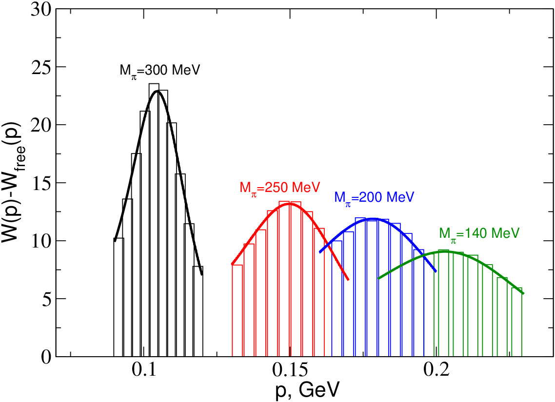
In case of the wide resonance like $\Delta$ , it is convenient to consider the so-called subtracted probability distribution, which is obtained from $W(p)$ by subtracting the background $W_{free}(p)$ corresponding to the free $\pi N$ pairs with $\delta(p)=0$ [45]. In the vicinity of the resonance, the subtracted distribution approximately follows the Breit-Wigner form of the scattering cross section and thus allows one to easily identify the resonance from the data on the energy spectrum.

Using the values of the various LECs determined from the fit, and substituting the scattering phase given by Eq. (18) into Eq. (24), one may easily predict the shape of the probability distributions at different values of the pion mass. The results are given in Fig. 7. It is seen that the distributions behave in the expected manner: for the higher pion masses, the center-of-mass momentum decreases and the distribution becomes narrower. Slightly after $300~\mbox{MeV}$ the distribution degenerates into the $\delta$ -function – the $\Delta$ resonance becomes stable. Of course, such a behavior can be only observed in practice, provided there are at least few data points with different values of $L$ at a given quark mass [45].

5 Conclusions

Here, we summarize the pertinent results of our study:

i)

We have calculated the ground state energy of the $\Delta$ resonance in a finite volume up-to-and-including $O(\epsilon^{4})$ in the small scale expansion.
ii)

The obtained explicit expressions have been used to analyze the recent data on the nucleon and $\Delta$ spectrum, provided by the ETM collaboration [12]. It turns out that the finite volume corrections are sizable using the central value for the data point with the smallest quark mass. Even at the present accuracy, this correction should be taken into account.
iii)

It is checked that the numerical values for the correction at $O(\epsilon^{3})$ and at $O(\epsilon^{4})$ do not differ significantly.
iv)

We perform a simultaneous fit to the nucleon and $\Delta$ masses in the infinite volume. The values of the LECs obtained in a result of such a fit are stable. However, the convergence of the chiral expansion of the baryon masses in the infinite volume is rather poor, since we are still at relatively high values of the quark masses.
v)

The measurement of the energy spectrum at different volumes opens the possibility for the extraction of the decay width. To this end, we have proposed a procedure based on the consistency condition Eq. (20). This procedure can be used meaningfully, provided more accurate data points emerge below threshold.

Acknowledgments:

We would like to thank C. Alexandrou, Z. Fodor, J. Gasser, K. Jansen, Ch. Lang, J. Negele, V. Pascalutsa, O. Pène, M. Procura, G. Schierholz, M. Vanderhaeghen and U. Wenger for interesting discussions. We acknowledge the support of the European Community-Research Infrastructure Integrating Activity “Study of Strongly Interacting Matter” (acronym HadronPhysics2, Grant Agreement n. 227431) under the Seventh Framework Programme of the EU. Work supported in part by DFG (SFB/TR 16, “Subnuclear Structure of Matter”), and by the Helmholtz Association through funds provided to the virtual institute “Spin and strong QCD” (VH-VI-231).

Appendix A The masses of the nucleon and the $\Delta(1232)$

A straightforward calculation of the nucleon and $\Delta$ masses at fourth order yields

$\displaystyle M_{N}$	$\displaystyle=$	$\displaystyle m_{N}-\frac{3g_{A}^{2}M^{3}}{32\pi F^{2}}-\frac{3g_{A}^{2}M^{4}}{64\pi^{2}F^{2}m_{N}}\,\biggl(2\ln\frac{M}{m_{N}}+1\biggr)+\frac{3M^{4}c_{2}}{128\pi^{2}F^{2}}$	(A.1)
	$\displaystyle+$	$\displaystyle\frac{3M^{4}(8c_{1}-c_{2}-4c_{3})}{32\pi^{2}F^{2}}\,\ln\frac{M}{m_{N}}+\frac{M^{4}}{48\pi^{2}F^{2}m_{N}m_{\Delta}^{2}}\,\biggl\{P_{1}+2P_{2}\ln\frac{M}{m_{N}}\biggr\}$
	$\displaystyle-$	$\displaystyle Z\,\frac{((m_{\Delta}+m_{N})^{2}-M^{2})\lambda(m_{\Delta}^{2},m_{N}^{2},M^{2})}{6m_{N}F^{2}m_{\Delta}^{2}}\,W_{\Delta}^{r}(m_{N}^{2})$
	$\displaystyle-$	$\displaystyle Z\,\frac{(m_{\Delta}-m_{N})(m_{\Delta}+m_{N})^{3}}{96\pi^{2}F^{2}m_{N}m_{\Delta}^{2}}\biggl\{\frac{(m_{\Delta}^{2}-m_{N}^{2})^{2}}{6m_{N}^{2}}-2M^{2}\ln\frac{M}{m_{N}}$
	$\displaystyle-$	$\displaystyle\frac{M^{2}(2m_{\Delta}^{2}+2m_{N}^{2}-m_{\Delta}m_{N})}{3m_{N}^{2}}\biggr\}+O(\epsilon^{5})\,,$

$\displaystyle M_{\Delta}$	$\displaystyle=$	$\displaystyle m_{\Delta}-\frac{5g_{1}^{2}M^{3}}{96\pi F^{2}}-\frac{5g_{1}^{2}M^{4}}{192\pi^{2}F^{2}m_{\Delta}}\,\biggl(\frac{20}{9}\,\ln\frac{M}{m_{N}}+\frac{49}{54}\biggr)+\frac{3M^{4}a_{2}}{128\pi^{2}F^{2}}$	(A.2)
	$\displaystyle+$	$\displaystyle\frac{3M^{4}(8a_{1}-a_{2}-4a_{3})}{64\pi^{2}F^{2}}\,2\ln\frac{M}{m_{N}}+\frac{M^{4}}{768\pi^{2}F^{2}m_{\Delta}^{5}}\,\biggl\{Q_{1}+2Q_{2}\ln\frac{M}{m_{N}}\biggr\}$
	$\displaystyle-$	$\displaystyle Z\,\frac{((m_{\Delta}+m_{N})^{2}-M^{2})\lambda(m_{\Delta}^{2},m_{N}^{2},M^{2})}{24m_{\Delta}^{3}F^{2}}\,W_{N}^{r}(m_{\Delta}^{2})$
	$\displaystyle-$	$\displaystyle Z\,\frac{(m_{\Delta}-m_{N})(m_{N}+m_{\Delta})^{3}}{384\pi^{2}F^{2}m_{\Delta}^{3}}\,\biggl\{\frac{(m_{\Delta}^{2}-m_{N}^{2})^{2}}{3m_{\Delta}^{2}}+2M^{2}\ln\frac{M}{m_{N}}$
	$\displaystyle-$	$\displaystyle\frac{2M^{2}(2m_{\Delta}^{2}+2m_{N}^{2}-m_{\Delta}m_{N})}{3m_{\Delta}^{2}}\biggr\}+O(\epsilon^{5})\,,$

where $M^{2}=2B\hat{m}$ and the “tree-level masses” are given by

$\displaystyle m_{N}$	$\displaystyle=$	$\displaystyle\mathring{m}_{N}-4c_{1}M^{2}-4B_{23}\Delta_{0}M^{2}-B_{32}\Delta_{0}^{3}-E_{1}\Delta_{0}^{4}-4E_{2}\Delta_{0}^{2}M^{2}-4e_{1}M^{4}$
	$\displaystyle=$	$\displaystyle\hat{\mathring{m}}_{N}-4\hat{c}_{1}M^{2}-4e_{1}M^{4}\,,$
$\displaystyle m_{\Delta}$	$\displaystyle=$	$\displaystyle\mathring{m}_{\Delta}-4a_{1}M^{2}-4B_{1}^{\Delta}\Delta_{0}M^{2}-B_{0}^{\Delta}\Delta_{0}^{3}-E_{1}^{\Delta}\Delta_{0}^{4}-4E_{2}^{\Delta}\Delta_{0}^{2}M^{2}-4e_{1}^{\Delta}M^{4}$	(A.3)
	$\displaystyle=$	$\displaystyle\hat{\mathring{m}}_{\Delta}-4\hat{a}_{1}M^{2}-4e_{1}^{\Delta}M^{4}\,,$	(A.3)

where $e_{1}=4e_{38}+\frac{1}{2}\,(e_{115}+e_{116})$ and $e_{1}^{\Delta}=4e_{38}^{\Delta}+\frac{1}{2}\,(e_{115}^{\Delta}+e_{116}^{\Delta})$ . Furthermore,

	$\displaystyle Z$	$\displaystyle=$	$\displaystyle c_{A}^{2}+2(m_{\Delta}-m_{N})c_{A}b_{3}+\frac{m_{\Delta}^{2}-m_{N}^{2}-M^{2}}{m_{N}}\,c_{A}b_{6}$		(A.4)
		$\displaystyle=$	$\displaystyle c_{A}^{2}+2\Delta_{0}c_{A}(b_{3}+b_{6})+O(\epsilon^{2})\,,$		(A.4)

and

$\displaystyle P_{1}$	$\displaystyle=$	$\displaystyle\frac{m_{N}+m_{\Delta}}{2m_{N}^{2}}\,\biggl\{\frac{c_{A}^{2}}{3}(-3m_{\Delta}^{3}-3m_{\Delta}m_{N}^{2}+8m_{N}^{3})$
	$\displaystyle-$	$\displaystyle(3m_{N}^{4}+2m_{\Delta}(m_{\Delta}^{2}+m_{N}^{2})(m_{\Delta}-m_{N}))c_{A}\biggl(b_{3}+\frac{m_{N}+m_{\Delta}}{2m_{N}}\,b_{6}\biggr)\biggr\}\,,$
$\displaystyle P_{2}$	$\displaystyle=$	$\displaystyle c_{A}^{2}(-m_{\Delta}^{2}+m_{N}^{2}+3m_{\Delta}m_{N})$
	$\displaystyle-$	$\displaystyle(m_{\Delta}+m_{N})(3m_{N}^{2}+2m_{\Delta}^{2}-2m_{\Delta}m_{N})c_{A}\biggl(b_{3}+\frac{m_{N}+m_{\Delta}}{2m_{N}}\,b_{6}\biggr)\,,$
$\displaystyle Q_{1}$	$\displaystyle=$	$\displaystyle c_{A}^{2}(3m_{\Delta}^{4}+4m_{N}^{4}+4m_{N}^{3}m_{\Delta}+4m_{N}^{2}m_{\Delta}^{2}+4m_{N}m_{\Delta}^{3})$
	$\displaystyle-$	$\displaystyle(m_{N}+m_{\Delta})\biggl(2c_{A}b_{3}+\frac{(m_{\Delta}+m_{N})c_{A}b_{6}}{m_{N}}\biggr)$
	$\displaystyle\times$	$\displaystyle(3m_{\Delta}^{4}+4m_{N}(m_{N}^{2}+m_{\Delta}^{2})(m_{N}-m_{\Delta}))\,,$

	$\displaystyle Q_{2}$	$\displaystyle=$	$\displaystyle-2m_{\Delta}^{2}\biggl\{c_{A}^{2}(2m_{N}m_{\Delta}+3m_{\Delta}^{2}+2m_{N}^{2})$
		$\displaystyle-$	$\displaystyle(m_{N}+m_{\Delta})\biggl(2c_{A}b_{3}+\frac{(m_{\Delta}+m_{N})c_{A}b_{6}}{m_{N}}\biggr)(-2m_{N}m_{\Delta}+3m_{\Delta}^{2}+2m_{N}^{2})\biggr\}\,.$

The loop functions are given by

	$\displaystyle W_{\Delta}^{r}(m_{N}^{2})$	$\displaystyle=$	$\displaystyle\left\{\begin{array}[]{l l}-\frac{\sqrt{-\lambda}}{16\pi^{2}m_{N}^{2}}\arccos\biggl(-\frac{m_{N}^{2}-m_{\Delta}^{2}+M^{2}}{2m_{N}M}\biggr)&\\[5.69054pt] -\frac{m_{N}^{2}-m_{\Delta}^{2}+M^{2}}{32\pi^{2}m_{N}^{2}}\,\biggl(2\ln\frac{M}{m_{N}}-1\biggr)\,,&\mbox{if $\lambda<0$}\\[22.76219pt] -\frac{\sqrt{\lambda}}{32\pi^{2}m_{N}^{2}}\,\ln\frac{m_{N}^{2}+M^{2}-m_{\Delta}^{2}+\sqrt{\lambda}}{m_{N}^{2}+M^{2}-m_{\Delta}^{2}-\sqrt{\lambda}}&\\[5.69054pt] -\frac{m_{N}^{2}-m_{\Delta}^{2}+M^{2}}{32\pi^{2}m_{N}^{2}}\,\biggl(2\ln\frac{M}{m_{N}}-1\biggr)\,,&\mbox{if $\lambda>0$}\\ \end{array}\right.\,,$
	$\displaystyle W_{N}^{r}(m_{\Delta}^{2})$	$\displaystyle=$	$\displaystyle\left\{\begin{array}[]{l l}-\frac{\sqrt{-\lambda}}{16\pi^{2}m_{\Delta}^{2}}\arccos\biggl(-\frac{m_{\Delta}^{2}-m_{N}^{2}+M^{2}}{2m_{\Delta}M}\biggr)&\\[5.69054pt] -\frac{m_{\Delta}^{2}-m_{N}^{2}+M^{2}}{32\pi^{2}m_{\Delta}^{2}}\,\biggl(2\ln\frac{M}{m_{N}}-1\biggr)\,,&\mbox{if $\lambda<0$}\\[22.76219pt] -\frac{\sqrt{\lambda}}{32\pi^{2}m_{\Delta}^{2}}\,\ln\frac{m_{\Delta}^{2}+M^{2}-m_{N}^{2}+\sqrt{\lambda}}{m_{\Delta}^{2}+M^{2}-m_{N}^{2}-\sqrt{\lambda}}&\\[5.69054pt] -\frac{m_{\Delta}^{2}-m_{N}^{2}+M^{2}}{32\pi^{2}m_{\Delta}^{2}}\,\biggl(2\ln\frac{M}{m_{N}}-1\biggr)\,,&\mbox{if $\lambda>0$}\\ \end{array}\right.\,,$

where $\lambda=\lambda(m_{\Delta}^{2},m_{N}^{2},M^{2})$ .

We further express the quantity $M^{2}$ through the pion mass, according to

\displaystyle M^{2}

\displaystyle=

\displaystyle M_{\pi}^{2}\biggl\{1+\frac{M_{\pi}^{2}}{32\pi^{2}F^{2}}\,\biggl(\bar{l}_{3}+\ln\frac{\bar{M}_{\pi}^{2}}{M_{\pi}^{2}}\biggr)\biggr\}\,,

(A.16)

where $\bar{l}_{3}=2.9\pm 2.4$ is the $O(p^{4})$ LEC in the meson sector of chiral perturbation theory and $\bar{M}_{\pi}$ stands for the physical pion mass.

Finally, normalizing $M_{N}$ and $M_{\Delta}$ at $M_{\pi}=\bar{M}_{\pi}$ and neglecting higher-order terms in the $\epsilon$ -expansion, we obtain the equations (8) from section 2, where

$\displaystyle x_{1}$	$\displaystyle=$	$\displaystyle-4\hat{c}_{1}\,,$
$\displaystyle y_{1}$	$\displaystyle=$	$\displaystyle-4\hat{a}_{1}\,,$
$\displaystyle x_{2}$	$\displaystyle=$	$\displaystyle-\frac{3g_{A}^{2}}{32\pi F^{2}}\,,$
$\displaystyle y_{2}$	$\displaystyle=$	$\displaystyle-\frac{5g_{1}^{2}}{96\pi F^{2}}\,,$

	$\displaystyle x_{3}$	$\displaystyle=$	$\displaystyle-4e_{1}-\frac{3g_{A}^{2}}{64\pi^{2}F^{2}\bar{m}_{N}}+\frac{3c_{2}}{128\pi^{2}F^{2}}+\frac{1}{24\pi^{2}F^{2}\bar{m}_{N}}\,\biggl(\frac{c_{A}^{2}}{3}-\frac{3}{2}\,c_{A}\bar{m}_{N}(b_{3}+b_{6})\biggr)$
		$\displaystyle-$	$\displaystyle\frac{c_{1}}{8\pi^{2}F^{2}}\,\biggl(\bar{l}_{3}+\ln\frac{\bar{M}_{\pi}^{2}}{\bar{m}_{N}^{2}}\biggr)\,,$

$\displaystyle y_{3}$	$\displaystyle=$	$\displaystyle-4e_{1}^{\Delta}-\frac{5g_{1}^{2}}{192\pi^{2}F^{2}\bar{m}_{\Delta}}\cdot\frac{49}{54}+\frac{3a_{2}}{128\pi^{2}F^{2}}$
	$\displaystyle+$	$\displaystyle\frac{1}{768\pi^{2}F^{2}\bar{m}_{\Delta}}\,\biggl(19c_{A}^{2}-12c_{A}\bar{m}_{\Delta}(b_{3}+b_{6})\biggr)-\frac{a_{1}}{8\pi^{2}F^{2}}\,\biggl(\bar{l}_{3}+\ln\frac{\bar{M}_{\pi}^{2}}{\bar{m}_{N}^{2}}\biggr)\,,$
$\displaystyle x_{4}$	$\displaystyle=$	$\displaystyle-\frac{3g_{A}^{2}}{32\pi^{2}F^{2}\bar{m}_{N}}+\frac{3(8c_{1}-c_{2}-4c_{3})}{32\pi^{2}F^{2}}+\frac{1}{8\pi^{2}F^{2}\bar{m}_{N}}\,\biggl(c_{A}^{2}-2c_{A}\bar{m}_{N}(b_{3}+b_{6})\biggr)$
	$\displaystyle+$	$\displaystyle\frac{c_{1}}{4\pi^{2}F^{2}}\,,$
$\displaystyle y_{4}$	$\displaystyle=$	$\displaystyle-\frac{5g_{1}^{2}}{192\pi^{2}F^{2}\bar{m}_{\Delta}}\cdot\frac{20}{9}+\frac{3(8a_{1}-a_{2}-4a_{3})}{32\pi^{2}F^{2}}$	(A.17)
	$\displaystyle-$	$\displaystyle\frac{1}{192\pi^{2}F^{2}\bar{m}_{\Delta}}\biggl(7c_{A}^{2}-12c_{A}\bar{m}_{\Delta}(b_{3}+b_{6})\biggr)+\frac{a_{1}}{4\pi^{2}F^{2}}\,,$	(A.17)

and the “tree-level” masses $m_{N},m_{\Delta}$ are given by Eq. (9).

Finally, the loop functions in Eq. (8) are defined as

$\displaystyle\Phi_{N}(m_{N},m_{\Delta},M_{\pi}^{2})$	$\displaystyle=$	$\displaystyle\frac{((m_{\Delta}+m_{N})^{2}-M_{\pi}^{2})\lambda(m_{\Delta}^{2},m_{N}^{2},M_{\pi}^{2})}{6m_{N}m_{\Delta}^{2}}\,W_{\Delta}^{r}(m_{N}^{2})$
	$\displaystyle+$	$\displaystyle\frac{(m_{\Delta}-m_{N})(m_{\Delta}+m_{N})^{3}}{96\pi^{2}m_{N}m_{\Delta}^{2}}\biggl\{\frac{(m_{\Delta}^{2}-m_{N}^{2})^{2}}{6m_{N}^{2}}$
	$\displaystyle-$	$\displaystyle\frac{M_{\pi}^{2}(2m_{\Delta}^{2}+2m_{N}^{2}-m_{\Delta}m_{N})}{3m_{N}^{2}}-2M_{\pi}^{2}\ln\frac{M_{\pi}}{m_{N}}\biggr\}\,,$
$\displaystyle\Phi_{\Delta}(m_{N},m_{\Delta},M_{\pi}^{2})$	$\displaystyle=$	$\displaystyle\frac{((m_{\Delta}+m_{N})^{2}-M_{\pi}^{2})\lambda(m_{\Delta}^{2},m_{N}^{2},M_{\pi}^{2})}{24m_{\Delta}^{3}}\,W_{N}^{r}(m_{\Delta}^{2})$	(A.18)
	$\displaystyle+$	$\displaystyle\frac{(m_{\Delta}-m_{N})(m_{N}+m_{\Delta})^{3}}{384\pi^{2}m_{\Delta}^{3}}\,\biggl\{\frac{(m_{\Delta}^{2}-m_{N}^{2})^{2}}{3m_{\Delta}^{2}}$
	$\displaystyle-$	$\displaystyle\frac{2M_{\pi}^{2}(2m_{\Delta}^{2}+2m_{N}^{2}-m_{\Delta}m_{N})}{3m_{\Delta}^{2}}+2M_{\pi}^{2}\ln\frac{M_{\pi}}{m_{N}}\biggr\}$

References

[1] D. G. Richards, M. Göckeler, R. Horsley, D. Pleiter, P. E. L. Rakow, G. Schierholz and C. M. Maynard [LHPC Collaboration], Nucl. Phys. Proc. Suppl. 109A (2002) 89 [arXiv:hep-lat/0112031].
[2] C. M. Maynard and D. G. Richards [UKQCD Collaboration], Nucl. Phys. Proc. Suppl. 119 (2003) 287 [arXiv:hep-lat/0209165].
[3] C. Gattringer et al. [BGR Collaboration], Nucl. Phys. B 677 (2004) 3 [arXiv:hep-lat/0307013]; D. Brömmel, P. Crompton, C. Gattringer, L. Y. Glozman, C. B. Lang, S. Schaefer and A. Schäfer [Bern-Graz-Regensburg Collaboration], Phys. Rev. D 69 (2004) 094513 [arXiv:hep-ph/0307073].
[4] S. Sasaki, T. Blum and S. Ohta, Phys. Rev. D 65 (2002) 074503 [arXiv:hep- lat/0102010]; S. Sasaki, Prog. Theor. Phys. Suppl. 151 (2003) 143 [arXiv:nucl-th/0305014]; K. Sasaki and S. Sasaki, Phys. Rev. D 72 (2005) 034502 [arXiv:hep-lat/0503026]; K. Sasaki, S. Sasaki and T. Hatsuda, Phys. Lett. B 623 (2005) 208 [arXiv:hep-lat/0504020].
[5] J. M. Zanotti et al. [CSSM Lattice Collaboration], Phys. Rev. D 65 (2002) 074507 [arXiv:hep-lat/0110216]; J. M. Zanotti, D. B. Leinweber, A. G. Williams, J. B. Zhang, W. Melnitchouk and S. Choe [CSSM Lattice collaboration], Phys. Rev. D 68 (2003) 054506 [arXiv:hep-lat/0304001].
[6] B. G. Lasscock, J. N. Hedditch, W. Kamleh, D. B. Leinweber, W. Melnitchouk, A. G. Williams and J. M. Zanotti, Phys. Rev. D 76 (2007) 054510 [arXiv:0705.0861 [hep-lat]].
[7] W. Melnitchouk et al., Phys. Rev. D 67 (2003) 114506 [arXiv:hep-lat/0202022].
[8] L. Zhou and F. X. Lee, Phys. Rev. D 74 (2006) 034507 [arXiv:hep-lat/0604023].
[9] N. Mathur et al., Phys. Lett. B 605 (2005) 137 [arXiv:hep-ph/0306199].
[10] D. Guadagnoli, M. Papinutto and S. Simula, Phys. Lett. B 604 (2004) 74 [arXiv:hep-lat/0409011].
[11] C. Alexandrou et al. [ETM Collaboration], PoS LAT2007 (2007) 087 [arXiv:0710.1173 [hep-lat]].
[12] C. Alexandrou et al. [European Twisted Mass Collaboration], Phys. Rev. D 78 (2008) 014509 [arXiv:0803.3190 [hep-lat]].
[13] C. McNeile, arXiv:hep-lat/0307027.
[14] D. B. Leinweber, W. Melnitchouk, D. G. Richards, A. G. Williams and J. M. Zanotti, Lect. Notes Phys. 663 (2005) 71 [arXiv:nucl-th/0406032].
[15] C. Gattringer, arXiv:0711.0622 [hep-lat].
[16] C. Alexandrou et al., arXiv:0810.3976 [hep-lat].
[17] N. Mathur et al., arXiv:0811.1400 [hep-lat].
[18] C. Morningstar, arXiv:0810.4448 [hep-lat].
[19] S. Dürr et al, Science 322 (2008) 1224.
[20] R. W. Gothe [CLAS Collaboration], AIP Conf. Proc. 814 (2006) 278; M. Battaglieri [CLAS Collaboration], AIP Conf. Proc. 964 (2007) 14.
[21] R. Beck, “Recent Results on Hadron Spectroscopy from ELSA and MAMI,” U. Thoma, “Recent results from baryon spectroscopy,” talks given ar XII. International Conference on Hadron Spectroscopy (Hadron07), LNF-INFN, 8-13 October 2007.
[22] M. Lüscher, Commun. Math. Phys. 105 (1986) 153.
[23] M. Lüscher, Nucl. Phys. B 354 (1991) 531.
[24] M. Lüscher, Nucl. Phys. B 364 (1991) 237.
[25] M. Lüscher, DESY-88-156 Lectures given at Summer School ’Fields, Strings and Critical Phenomena’, Les Houches, France, Jun 28 - Aug 5, 1988
[26] U.-J. Wiese, Nucl. Phys. Proc. Suppl. 9 (1989) 609.
[27] T. A. DeGrand, Phys. Rev. D 43 (1991) 2296.
[28] K. Rummukainen and S. A. Gottlieb, Nucl. Phys. B 450 (1995) 397 [arXiv:hep-lat/9503028].
[29] C. H. Kim, C. T. Sachrajda and S. R. Sharpe, Nucl. Phys. B 727 (2005) 218 [arXiv:hep-lat/0507006].
[30] N. H. Christ, C. Kim and T. Yamazaki, Phys. Rev. D 72 (2005) 114506 [arXiv:hep-lat/0507009].
[31] S. Aoki et al. [CP-PACS Collaboration], Phys. Rev. D 76 (2007) 094506 [arXiv:0708.3705 [hep-lat]].
[32] M. Göckeler, R. Horsley, Y. Nakamura, D. Pleiter, P. E. L. Rakow, G. Schierholz and J. Zanotti, arXiv:0810.5337 [hep-lat].
[33] S. R. Beane, P. F. Bedaque, A. Parreno and M. J. Savage, Nucl. Phys. A 747 (2005) 55 [arXiv:nucl-th/0311027].
[34] S. R. Beane, P. F. Bedaque, A. Parreno and M. J. Savage, Phys. Lett. B 585 (2004) 106 [arXiv:hep-lat/0312004].
[35] S. R. Beane, P. F. Bedaque, T. C. Luu, K. Orginos, E. Pallante, A. Parreno and M. J. Savage [NPLQCD Collaboration], Nucl. Phys. A 794 (2007) 62 [arXiv:hep-lat/0612026].
[36] S. R. Beane, P. F. Bedaque, K. Orginos and M. J. Savage, Phys. Rev. Lett. 97 (2006) 012001 [arXiv:hep-lat/0602010].
[37] S. Sasaki and T. Yamazaki, Phys. Rev. D 74 (2006) 114507 [arXiv:hep-lat/0610081].
[38] C. Michael, Nucl. Phys. B 327 (1989) 515.
[39] R. D. Loft and T. A. DeGrand, Phys. Rev. D 39 (1989) 2692.
[40] L. Lellouch and M. Lüscher, Commun. Math. Phys. 219 (2001) 31 [arXiv:hep-lat/0003023].
[41] T. Yamazaki and N. Ishizuka, Phys. Rev. D 67 (2003) 077503 [arXiv:hep-lat/0210022].
[42] E. Jenkins and A. V. Manohar, Phys. Lett. B 259 (1991) 353.
[43] T. R. Hemmert, B. R. Holstein and J. Kambor, J. Phys. G 24 (1998) 1831 [arXiv:hep-ph/9712496].
[44] V. Bernard, U.-G. Meißner and A. Rusetsky, Nucl. Phys. B 788 (2008) 1 [arXiv:hep-lat/0702012].
[45] V. Bernard, M. Lage, U.-G. Meißner and A. Rusetsky, Eur. Phys. J. A 35 (2008) 281; V. Bernard, M. Lage, U.-G. Meißner and A. Rusetsky, JHEP 0808 (2008) 024
[arXiv:0806.4495 [hep-lat]].
[46] A. Ali Khan et al. [QCDSF-UKQCD Collaboration], Nucl. Phys. B 689 (2004) 175 [arXiv:hep-lat/0312030].
[47] V. Bernard, T. R. Hemmert and U.-G. Meißner, Phys. Lett. B 622 (2005) 141 [arXiv:hep-lat/0503022];
[48] V. Bernard, T. R. Hemmert and U.-G. Meißner, Phys. Lett. B 565 (2003) 137 [arXiv:hep-ph/0303198].
[49] H. B. Tang and P. J. Ellis, Phys. Lett. B 387 (1996) 9 [arXiv:hep-ph/9606432].
[50] P. J. Ellis and H. B. Tang, Phys. Rev. C 56, 3363 (1997) [arXiv:hep-ph/9609459].
[51] N. Fettes and U.-G. Meißner, Nucl. Phys. A 679 (2001) 629 [arXiv:hep-ph/0006299].
[52] V. Bernard, Prog. Part. Nucl. Phys. 60 (2008) 82 [arXiv:0706.0312 [hep-ph]].
[53] H. Krebs, E. Epelbaum and U.-G. Meißner, Eur. Phys. J. A 32 (2007) 127 [arXiv:nucl-th/0703087].
[54] M. Procura, B. U. Musch, T. Wollenweber, T. R. Hemmert and W. Weise, Phys. Rev. D 73 (2006) 114510 [arXiv:hep-lat/0603001].
[55] B. C. Tiburzi and A. Walker-Loud, Nucl. Phys. A 764 (2006) 274 [arXiv:hep-lat/0501018].
[56] V. Pascalutsa and M. Vanderhaeghen, Phys. Lett. B 636 (2006) 31
[arXiv:hep-ph/0511261].
[57] J. Gasser, V. E. Lyubovitskij and A. Rusetsky, Phys. Rept. 456 (2008) 167
[arXiv:0711.3522 [hep-ph]].
[58] A. Walker-Loud et al., arXiv:0806.4549 [hep-lat].