Monitoring the wave function by time continuous position measurement
Abstract
We consider a single copy of a quantum particle moving in a potential and show that it is possible to monitor its complete wave function by only continuously measuring its position. While we assume that the potential is known, no information is available about its state initially. In order to monitor the wave function, an estimate of the wave function is propagated due to the influence of the potential and continuously updated according to the results of the position measurement. We demonstrate by numerical simulations that the estimation reaches arbitrary values of accuracy below within a finite time period for the potentials we study. In this way our method grants, a certain time after the beginning of the measurement, an accurate real-time record of the state evolution including the influence of the continuous measurement. Moreover, it is robust against sudden perturbations of the system as for example random momentum kicks from environmental particles, provided they occur not too frequently.
Monitoring - continuous observation - of a dynamical system in the presence of randomness is employed not only in physics and chemistry, e.g., to survey the motion of comets, the growth of thin layers or the dynamics of chemical reactions. It is a sub-discipline of robotics and also plays a vital role in other fields such as earth sciences and aeronautics with numerous applications from climate observation, control of robots and vehicles to remote sensing. Monitoring tasks can be modeled by stochastic processes supported by continuous updates of estimates according to the observed random data - also called stochastic filtering [1]. A special challenge, however, is posed in the realm of quantum physics; the preparation - not to mention monitoring or control - of individual atoms, electrons and photons remained experimentally unattainable for half a century. The theory of quantum monitoring only emerged 20 years ago [2, 3, 4, 5]. Nowadays, however, nano-technology and quantum information processing strongly inspire a mathematical theory of monitoring and control of single quantum degrees of freedom like, e.g., the position of an atom or a nano-object. A more challenging aim is to monitor and control the entire state of individual quantum systems.
Monitoring a quantum system encounters principle difficulties that lie in the characteristic traits of quantum nature itself: incompatible observables such as position and momentum and irreversible state change introduced by measurements. Methods have been developed to employ monitoring in order to determine the pre-measurement state [6], for parameter estimation [7], to track Rabi oscillations [8, 9, 10] and -combined with feedback- for cooling purposes [11] or to reach a targeted state [12]. Moreover, the possibility of state monitoring has been studied for special systems [13, 14]. We are here going to show, that monitoring the position of a single quantum particle promises - via our theory - the monitoring of the full wave function, i.e., the complete state of a particle, and demonstrate its power by numerical simulations. Like always in the quantum realm, monitoring will unavoidably alter the original (unmonitored) evolution of the wave function. Strong monitoring assures very robust fidelity of the estimated wave function but it has little to do with the unmonitored wave function. Fortunately, in many cases, a suitable strength of monitoring assures both robust fidelity and slight change of self-dynamics. Needless to say, that such compromise is not due to any weakness in our theory. It is definitely an ultimate necessity enforced by the Heisenberg uncertainty relations.
In the following the concept of continuous observation is interpreted as the asymptotic limit of dense sequences of unsharp position measurements on a single quantum particle. We describe the inference of its wave function from the sequence of the measured position data and eventually compare the true wave function with its estimate using simulations of quantum particles moving in various potentials. Among them is the Hénon-Heiles potential, which in classical physics implies chaotic behaviour and thus exposes tracking of dynamics to extreme conditions.
I Monitoring the position
Time-continuous position measurement can be understood as an idealization of a sequence of discrete unsharp position measurements carried out consecutively on a single copy of a quantum particle [3]. The notion of unsharp measurement is instrumental here. Such an unsharp measurement of the position can be realized as indirect von Neumann measurement; instead of measuring the particle’s position directly, an ancilla system is scattered off the particle and then the ancilla is measured [15, 16, 17, 18, 19]. The observed results yield limited information on the position of the scatterer. In a simple description, a single unsharp measurement of resolution collapses the wave function onto a neighborhood with characteristic extent of a random value :
| (1) |
where is a central Gaussian function. The random quantity is the measured position which determines the collapse, i.e., the weighted projection, of the wave function. The probability to obtain the measurement result - which also plays the role of the normalization factor of the post-measurement wave function - reads:
| (2) |
As a matter of fact, sharp (direct) von Neumann position measurements are the idealized special case while unsharp measurements - though not necessarily with the Gaussian profile - are the ones which we encounter in practice and which suite a tractable theory of real-time monitoring of the position of a single quantum particle.
In our discretized model of monitoring a single particle, we assume an unknown initial wave function and we are performing consecutive unsharp position measurements of resolution at times , resp., yielding the corresponding sequence of measurement outcomes. Between two consecutive unsharp measurements the wave function evolves according to its Schrödinger equation (self-dynamics).
The resolution and the frequency of unsharp measurements should be chosen in such a way as not to heavily distort the self-dynamics of the particle. It turns out that the relevant parameter is , we call
| (3) |
the strength of position monitoring. If stands for the characteristic extension of the wave function, then is the average decoherence rate at which our monitoring distorts the monitored particle’s self-dynamics. We should keep this rate modest compared to the rate of the Schrödinger evolution due to the Hamiltonian of the monitored particle. Low values of the strength may, however, result in low efficiency of position monitoring and slow convergence of our method of wave function estimation, cp. Sec III. The above constraints on can in general be matched with further ones - see Sec. IV - that assure the applicability of the continuous limit and its analytic equations.
II Monitoring the wave function
While it seems plausible that after a sufficiently long time the sequence of unsharp position measurements provides enough data to estimate , it may come as surprise that position measurements enable a faithful monitoring of the full wave function as well. Let’s just outline the reason. Measuring the position at times on an system with evolving Schrödinger wave function is equivalent to consecutive measurements of the Heisenberg observables on a system with static wave function . The set of Heisenberg coordinates will exhaust a sufficiently large space of incompatible observables so that their measurements will lead to a faithful determination of and - this way - to our faithful determination of for long enough times . In the degenerate case , monitoring turns out to be trivial: For long enough times, a large number of unsharp position measurements of resolution is equivalent with a single sharp measurement of resolution , position monitoring thus yields just preparation of a static sharply localized wave function - an approximate ‘eigenstate’ of .
Our monitoring of the wave function means a real-time estimation of it, where the quality of monitoring depends on the fidelity of the estimation. We start from a certain initial estimate and simulate its evolution according to the self-dynamics of the particle, which is assumed to be known, until time . Immediately after we have learned the first position from the first measurement on the particle, we update the estimate according to the same rule (1) as the actual wave function of the particle and renormalize it:
| (4) |
This update resembles the Bayes principle of non-parametric statistical estimation. We repeat this procedure for to expect that the estimated and the observed wave function will converge! A rigorous proof of convergence is missing. In the continuous limit, nonetheless, it has been proved for the general case [20] - not excluding the lack of convergence in specific degenerate cases when the set of Heisenberg observables remains too narrow to determine . This is the case for example for a two-dimensional separable dynamics in two coordinates , where only the coordinate is monitored. Rather than pursuing the rigorous theoretical conditions of convergence cf. [21], we turned to numerical tests of continuous measurements that have definitely confirmed our method.
III Numerical Simulations
We simulated the evolution of a single hydrogen atom subject to continuous measurements in several potentials. However, the conclusions of our discussion are not restricted to hydrogen atoms; similar results can be expected for atoms with higher masses in appropriately scaled potentials.
The coupled evolutions of wave function, measurement readout and the estimated wave function were simulated numerically by discretizing the corresponding stochastic differential equations (cp. Sec.IV). For this purpose we employed a corresponding scheme of Kloeden and Platen which is accurate up to second order in the time step of the discretization [22, 18].
In order to study the relation between the evolution of the wave function of the particle on one hand and the evolution of its estimate on the other hand we first restrict to a one-dimensional spatial motion. In this case the graphical representation is the simplest and thus gives a clear picture of the convergence between real and estimated wave functions. As example we consider a hydrogen atom situated in a quartic double well potential with a shape as depicted in Fig.1.
We assumed a continuous measurement of the position of the hydrogen atom with strength . In order to get an impression of the dimensions of the measurement, let us invoke Eq. (3) to note that this value of may correspond, e.g., to single Gaussian measurements with spatial resolution of mm repeated at time periods ns. The spatial resolution of the single weak measurements [23] is thus times poorer than the width m of the initial Gaussian wave function of the atom.

In Fig.1 we have depicted snapshots recorded at different times of the spatial probability density of the H-atom (blue solid line) and the squared modulus of the estimated wave function (red dashed line). Initially both probability densities assume the form of Gaussians which differ in width and location within the double-well potential. The sequence of pictures demonstrates the convergence of the densities in the course of a continuous measurement.
The real probability density of the H-Atom, which possesses initially a slightly higher mean energy than the middle peak of the potential, oscillates back and forth between the sides of the potential. The oscillatory motion of the centre of would also be expected qualitatively without measurements -as well as from a classical particle of the same mass moving in the double well. However, the real probability density does not spread as it would do without measurements. This localisation effect caused by the continuous unsharp position measurement adapts the motion of the H-Atom to that of a classical particle which is perfectly localised at each instance. This illustrates the influence of the measurements and points to a particular kind of control of the wave function that can be exercised by means of unsharp position measurements. A smaller measurement strength would lead to less disturbance of the unitary motion in the potential but also to less speed of convergence between real and estimated probability density.
The estimated probability density , which is centered initially on the right-hand side of the potential, follows the real wave function until after approximately one oscillation period the corresponding probability densities coincide and evolve identically thereafter. But not only the probabilities to find the atom at a certain position converge, in fact the complete wave function and its estimate coincide after a sufficiently long period! It can be proved analytically, that the estimation fidelity , which measures the overlap between the wave functions and , when averaged over many realisations of the continuous measurement increases with time and converges to [20]. Numerical simulations for the double-well potential show that in a typical realisation with initial values as described above and measurement strength the fidelity amounts to more than after oscillation periods.
Fig.2 shows the evolution of estimation fidelity for of a continuously measured H-atom moving in a plane under the influence of a mexican-hat potential. The latter is a rotationally symmetric version of the double well in two spatial dimensions. For the sake of simplicity we assumed that both position coordinates are simultaneously and independently measured with the same strength . Such a continuous measurement of both coordinates typically yields evolutions of the estimation fidelities which are shown in Fig.2 for several values of the measurement strength . In all depicted cases the fidelity comes very close to one within a period of ms, i.e., estimated and real wave function then coincide. Thereafter the dynamics of the wave function including the influence of the measurement can thus be monitored with perfect fidelity.

One might doubt that our monitoring remains efficient for heavily complex wave functions like those developing in classically chaotic systems. Instead of the integrable Mexican hat potential, this time we study the chaotic Hénon-Heiles potential which depends on the radius as well as on the azimuth :
| (5) |
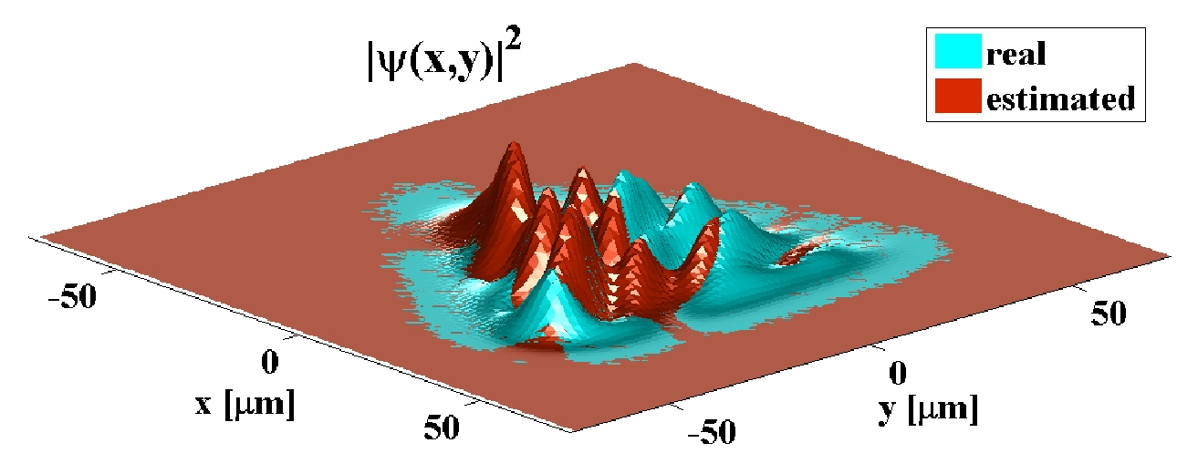
For this potential we simulated continuous position measurement and monitoring with the following results. The saturation of fidelity is reassuring: the estimate converges to the real wave function (Fig.3), which is found at a just slightly longer time scale than in the integrable Mexican hat potential, whereas the wave functions show an apparently irregular complex structure. Fig.4 shows the estimate and the real wave functions with an average overlap (i.e. a fidelity) of 91.58%. Indicating already an accurate overall estimation of the real wave function, this value still includes in small areas of the potential differences of the corresponding probability densities up to 35% of their highest peak. In particular, Fig.4 indicates that faithful monitoring is not only possible when the shape of the wave function of the particle is close to a Gaussian but also for rather complex shapes.

Monitoring, i.e. continuous unsharp observation, has a specific capacity. It is its robustness against external unexpected perturbations. To demonstrate such a robustness, we assumed that close to saturation of the estimation fidelity, like in Fig.4, our atom in the Hénon-Heiles potential is suddenly perturbed, e.g., by a collision with an environmental particle (here another hydrogen atom). For simplicity, we assume a momentum kick along the x-direction which implies a multiplication of the real wave function by the complex function hence the estimated wave function has to start a new cycle of convergence. We map the momentum kick to a temperature by as if it had a thermal origin, just to give a hint of its strength. Numeric results (Fig.5) show that the estimation fidelity recovers against these momentum perturbations (cp. movie [24]). In realty, repeated random perturbations might prevent perfect monitoring and fidelity will saturate at less than . This case is beyond the scope of our present work, its study will be of immediate interest since real systems are subject to various noises that are not measured at all. The monitoring theory at non-optimum efficiency has been outlined earlier [20].

IV The Ito-method
The discrete sequence of unsharp measurements (1,2) and wave function updates (4) possess their continuous limit [25] if we take and at . In this ‘continuous limit’ both the true wave function and the estimated wave function become continuous stochastic processes such that they are tractable by two stochastic differential equations respectively. The position measurement outcomes do not yield a continuous stochastic process themselves. It is their time-integral , specified below, that becomes a continuous stochastic process.
Let us consider the discrete increment of the true wave function during the period , cf. (1). In Dirac formalism we get:
| (6) |
For simplicity, we omit notations of time dependence . The symbol stands for . In the continuous limit, the Eq. (6) transforms into the following Ito-stochastic differential equation [3]:
| (7) | |||||
The equation of the discrete increment of the estimate (slight change) assumes the same form as Eq. (6) of but the normalization factor differs from , cf. (4). Yet, it yields the same Ito-stochastic differential equation as the equation above. The estimated state must be evolved according to the same non-linear differential equation (7) that describes the evolution of the monitored particle’s state . These two equations are coupled via the stochastic process whose discrete increment is defined by , in the continuous limit this means formally where is the measured position at time . In realty, the random process is obtained from the measured data . If the measurement is just simulated, like in our work, then in the continuous limit transforms into the Ito-differential whose random evolution can be generated by the standard Wiener process via . Of course, breaks the symmetry between the stochastic processes and because fluctuates around and not around .
The stochastic differential equation (7) - combined with the same one for - is a suitable approximation of our discrete model (Secs. II-III) under two conditions: (i) a single measurement does not resolve any particular structure of the wave function, i.e., where is the width of the spatial area on which is not negligibly small. Thus can, e.g., be of the order of magnitude of the available width of the confining potential. (ii) The length of the time period between two consecutive measurements is small compared to the timescale of self-dynamics generated by the Hamiltonian . Then the discrete model of position monitoring and wave function estimation becomes tractable by the time-continuous equation (7) depending on the single parameter , cf. also Eq. (3).
V Summary
We simulated numerically continuous position measurements carried out on a single quantum particle in one- and two-dimensional potentials. In order to monitor the evolution of an initially unknown state of the particle in a known potential, we estimated its wave function and updated the estimate continuously employing the measurement results.
Our simulations show that for all considered potentials the overlap between estimated and real wave function comes close to after a finite period of measurement -guaranteeing thereafter precise knowledge of the particle’s state and a real-time monitoring of its further evolution with high fidelity. The power of our method is indicated by the ability to monitor even the motion of a particle in a classically chaotic potential subject to continuous position measurement.
We thus demonstrated, that monitoring the complete state of a quantum system with infinite dimensional state space is feasible by continuously measuring a single observable on a single copy of the system. Moreover, the simulations indicate that our monitoring method is robust against sudden external perturbations such as occasional random momentum kicks. How much and what kinds of external noise this monitoring scheme tolerates is important for its applicability in control and error correction tasks, and might be object of future research.
VI Acknowledgements
We gratefully acknowledge support by the Bilateral Hungarian-South African R&D Collaboration Project, Hungarian OTKA grant 49384 and South African NRF Focus Area grant 65579. We thank J. Audretsch and A. Scherer for discussions. In particular, we are grateful to Ronnie Kosloff for his idea to monitor chaotic dynamics as well.
References
- [1] R. E. Kalman, R. S. Bucy, Trans. ASME J. Basic Eng. Ser. D 83, 95 (1961).
- [2] V. P. Belavkin, Lect. Notes Contr. Inf. Sci. 121, 245 (1988).
- [3] L. Diósi, Phys. Lett. 129 A, 419 (1988).
- [4] H. M. Wiseman and G. J. Milburn, Phys. Rev. A47, 642 (1993).
- [5] H. Carmichael: An Open Systems Approach to Quantum Optics (Springer, Berlin, 1993).
- [6] A. Silberfarb, P. S. Jessen, and I. H. Deutsch, Phys. Rev. Lett. 95, 030402 (2005).
- [7] B. A. Chase and J. M. Geremia, arXiv:0811.0601v1 [quant-ph].
- [8] J. Audretsch, T. Konrad, and A.Scherer, Phys. Rev. A 63, 052102 (2001).
- [9] J. Audretsch, T. Konrad, and A.Scherer, Phys. Rev. A 65, 033814 (2002).
- [10] J. Audretsch, F.E. Klee, and T. Konrad, Phys. Lett. A 361, 212-217 (2007).
- [11] D. A. Steck, Phys. Rev. A 74, 012322 (2006).
- [12] A. Shabani and K. Jacobs, Phys. Rev. Lett. 101, 230403 (2008).
- [13] A. C. Doherty, S. M. Tan, A. S. Parkins, and D. F. Walls, Phys. Rev. A 60 2380 (1999).
- [14] N. P. Oxtoby, J. Gambetta, and H. M. Wiseman, Phys. Rev. B 77, 125304 (2008).
- [15] J. von Neumann: Mathematical Foundations of Quantum Mechanics (Princetion Univ. Press, Princeton, 1955).
- [16] C.M. Caves and G.J. Milburn, Phys. Rev. A36, 5543 (1987).
- [17] P.Busch, M. Grabowski and J.P.Lathi: Operational Quantum Physics (Springer Verlag, Heidelberg, 1995).
- [18] H.-P. Breuer and F. Petruccione: The Theory of Open Quantum Systems (Oxford Univ. Press, Oxford, 2002).
- [19] K. Jacobs and D. A. Steck, Contemporary Physics 47(5),279-303 (2006)
- [20] L. Diósi, T. Konrad, A. Scherer, and J. Audretsch, J. Phys. A: Math. Gen. 39, L575 (2006).
- [21] R. van Handel and H. Mabuchi, J. Opt. B: Quantum Semiclass. Opt. 7, S226 (2005).
- [22] P. E. Kloeden and E. Platen, Numerical Solution of Stochastic Differential Equations, Springer, 1992.
- [23] L. Diósi, in: Encyclopedia of Mathematical Physics, eds.: J.-P. Françoise, G. L. Naber, and S. T. Tsou (Elsevier, Oxford, 2006)
- [24] Animated simulation (movie). Download from: http://physics.ukzn.ac.za/~konrad/waveandfid.avi.
- [25] A. Barchielli, Phys. Rev. D34, 2527 (1986).