1Introduction

IPPP/09/03, DCPT/09/06, QMUL-PH-09-01

Two-Loop Polygon Wilson Loops in $\mathcal{N}=4$ SYM

C. Anastasiou^a, A. Brandhuber^b, P. Heslop^b, V. V. Khoze^c, B. Spence^b and G. Travaglini^b¹¹ 1 babis@phys.ethz.ch, valya.khoze@durham.ac.uk, { a.brandhuber, p.j.heslop, w.j.spence, g.travaglini}@qmul.ac.uk

^a

Institute for Theoretical Physics, ETH Zürich
8093 Zürich, Switzerland
^b

Centre for Research in String Theory
Department of Physics, Queen Mary, University of London
Mile End Road, London, E1 4NS, United Kingdom
^c

Institute for Particle Physics Phenomenology, Department of Physics,
Durham University, Durham, DH1 3LE, United Kingdom

Abstract

We compute for the first time the two-loop corrections to arbitrary $n$ -gon lightlike Wilson loops in ${\cal N}=4$ supersymmetric Yang-Mills theory, using efficient numerical methods. The calculation is motivated by the remarkable agreement between the finite part of planar six-point MHV amplitudes and hexagon Wilson loops which has been observed at two loops. At $n=6$ we confirm that the ABDK/BDS ansatz must be corrected by adding a remainder function, which depends only on conformally invariant ratios of kinematic variables. We numerically compute remainder functions for $n=7,8$ and verify dual conformal invariance. Furthermore, we study simple and multiple collinear limits of the Wilson loop remainder functions and demonstrate that they have precisely the form required by the collinear factorisation of the corresponding two-loop $n$ -point amplitudes. The number of distinct diagram topologies contributing to the $n$ -gon Wilson loops does not increase with $n$ , and there is a fixed number of “master integrals”, which we have computed. Thus we have essentially computed general polygon Wilson loops, and if the correspondence with amplitudes continues to hold, all planar $n$ -point two-loop MHV amplitudes in the ${\cal N}=4$ theory.

1 Introduction

A surprising feature encountered in the study of supersymmetric gauge theories is the existence of an intriguing iterative structure in the higher-loop expansion of the Maximally Helicity Violating (MHV) scattering amplitudes in planar $\mathcal{N}=4$ super Yang-Mills (SYM) theory. This iterative structure was first discovered by Bern, Dixon, Kosower and one of the present authors (ABDK) studying collinear limits of maximally supersymmetric gauge theory amplitudes, and in the planar four-point MHV amplitude at two loops [1]. In the same paper, it was also conjectured that the same iterative structure should hold for two-loop MHV amplitudes with an arbitrary number of external legs.

In a subsequent important development, Bern, Dixon and Smirnov (BDS) proposed an all-loop resummed formula for the $n$ -point MHV amplitude, which they were able to confirm in an impressive three-loop calculation of the four-point amplitude [2]. According to this conjecture, multi-loop amplitudes can be re-expressed in terms of the one-loop amplitude and four kinematic-independent functions of the ’t Hooft coupling. One of these functions is the cusp anomalous dimension [3, 4, 5], for which an all-order expression has been proposed in [6].

The ABDK/BDS conjecture was further investigated in several papers. In particular, it was confirmed in a two-loop calculation for the five-point amplitude in [7] -- a result which is particularly non-trivial since it implies a cancellation of certain parity-odd terms in the two-loop term of the logarithm of the amplitude.¹¹ 1 The iteration for the parity-even terms had been proved earlier in [8]. It was also pointed out in [9] that the amplitudes of the $\beta$ -deformed ${\cal N}=4$ theory with real $\beta$ are identical to those of the undeformed theory (modulo an irrelevant, overall phase), and as such they will satisfy the ABDK/BDS iterative structure if the corresponding undeformed amplitudes do. Explicit expressions of the four-point amplitudes at four and five loops were also derived in [10] and [11], respectively, and, for the four-dimensional cut-constructible part of the five-point amplitude at three loops in [12]; these expressions will allow for further tests of the BDS ansatz at four and five loops once the relevant integral functions have been evaluated to the necessary degree of accuracy in $\epsilon$ .

One of the key aspects of the ABDK/BDS conjecture is the appearance of the exponentiation of the one-loop result in the complete perturbative answer. In a remarkable paper [13], Alday and Maldacena succeeded in using the AdS/CFT correspondence to provide a string theory formalism to address scattering amplitudes at strong coupling. In particular, their calculation of the four-point amplitude reproduced the strong-coupling limit of the BDS ansatz. It also provided a string theory explanation for why planar scattering amplitudes at strong coupling exponentiate, through a semiclassical calculation. It was argued in [14] that the same exponentiation of [13] should hold not only for MHV amplitudes but also for non-MHV amplitudes, since the helicity dependence of the amplitudes in the prefactor is unlikely to modify the semiclassical exponent in the path integral. However, for the non-MHV case the exponentiation can only occur at strong coupling, and is not apparent in perturbation theory.

The result of [13] suggested that the vacuum expectation value of a polygonal $n$ -edged Wilson loop, evaluated this time at weak coupling, could be related to the perturbative $n$ -point MHV amplitude in $\mathcal{N}=4$ SYM [15, 16]. This was confirmed in a one-loop calculation for $n=4$ in [15] and subsequently for arbitrary $n$ in [16]. Drummond, Henn, Korchemsky and Sokatchev (DHKS) were later able to confirm this conjecture in a remarkable analytic calculation of the two-loop four-edged Wilson loop [17], followed by a semi-analytical calculation of the five-edged Wilson loop [18].

It was later argued [19] that the BDS ansatz may be incomplete, specifically for $n$ -point amplitudes with $n\geq 6$ [20]. The authors of [21] have carried out an explicit calculation which shows that the BDS ansatz indeed needs to be modified in order to reproduce the two-loop term of the logarithm of the six-point amplitude. In a parallel development, the corresponding six-point lightlike Wilson loop was computed at two loops in [22, 23], and compared in [21, 23] to the parity-even part of the amplitude evaluated in [21].²² 2 The full six-point amplitude at two loops has been presented in [24]. The result of this analysis is that the MHV amplitude, stripped of the tree-level prefactor, and the Wilson loop are in perfect agreement (up to an additive constant) for the two-loop, six-point case,³³ 3 More accurately, there is a difference in the coefficients of the subleading $1/\epsilon$ pole for the Wilson loop and the amplitude. We will come back to this point in Section 3.2. but there is an additional contribution compared to what the BDS ansatz predicts. This extra term, which we will refer to as the remainder function, will be one of the main characters of our paper.

The possibility of having a nonvanishing remainder function was neatly explained in [18] in terms of the anomalous conformal symmetry of the lightlike Wilson loop. In that paper the associated anomalous conformal Ward identities were derived, and it was shown that the BDS expression provided a particular solution to these Ward identities. At the same time, the anomalous Ward identities cannot uniquely determine terms that are invariant under the conformal symmetry, and this leaves room for a conformally invariant remainder function [18]. For $n\leq 5$ , the lightlike constraints on the particle momenta restrict such conformally invariant contributions to just (kinematic-independent) constants. However, starting from $n=6$ edges one can build functions of the conformally invariant ratios which are left undetermined by the Ward identities, and need no longer vanish. DHKS made the prediction therefore that, if the duality with Wilson loops holds, the remainder function should depend on the kinematics only through cross-ratios.

The dual conformal symmetry of the Wilson loop was also instrumental in suggesting that the $S$ -matrix of the ${\cal N}=4$ theory should possess a dual superconformal symmetry [25, 26], which is expected to be exact at tree level, and violated by an anomaly at the loop level. Indeed, it was later proved in [27] using a supersymmetric version [28, 27, 29] of the BCF recursion relation [30, 31] that the tree-level $S$ -matrix of the planar ${\cal N}=4$ theory is covariant under the dual superconformal symmetry. A solution of the supersymmetric recursion relation of [28, 27, 29] was also presented in [32]. We also mention that the dual superconformal charges resurface as part of an infinite tower of charges coming from integrability of the dual AdS sigma model [33, 34].

In this paper, we present the results of our study of the Wilson loop remainder function for arbitrary $n$ . One important observation is that the structure of infrared and other integrable singularities of the diagrams which enter the Wilson loop calculation does not change for $n>7$ . Therefore, with the same numerical routines we can evaluate Wilson loops for arbitrary $n$ . We should note that our calculations were performed for Euclidean kinematics, but a generalisation to Minkowskian kinematics is possible.

There are several interesting properties of the remainder functions which we have analysed. The first one is its conjectured dependence on the kinematics only through cross-ratios. In our study we have collected ample numerical evidence that confirms this expectation for $n=6,7$ and $8$ points. The second aspect is the study of simple and multiple collinear limits of this function. Specifically, using universal factorisation theorems [35, 36, 37, 38] for scattering amplitudes one can predict [21] the behaviour of the $n$ -point amplitude remainder functions under simple collinear limits, namely ${\cal R}_{n}\to{\cal R}_{n-1}$ . In this paper we will show that the appropriately defined Wilson loop remainder function ${\cal R}_{n}^{\mathrm{WL}}$ has exactly the same collinear behaviour, namely

{\cal R}_{n}^{\mathrm{WL}}\,\to\,{\cal R}_{n-1}^{\mathrm{WL}}\ .

(1.1)

Notice that no additional constant term appears on the right hand side of (1.1). We have checked this numerically for $n=6,7$ and $8$ sided polygon Wilson loops. Finally, one of the most important goals for the future is to find analytic expressions for the remainder functions. As a first step we have initiated a detailed map of these functions, in particular for $n=6$ , for a wide range of values of the cross-ratios. We were able to make intriguing observations for special values of the cross-ratios and lower dimensional slices of the kinematic parameter spaces. On general grounds, we expect the remainder functions to be transcendentality four functions of the conformal cross-ratios. However, even if we restrict the remainder functions to a one-dimensional slice of the parameter space, the space of transcendentality four functions is rather large and, hence, numerical methods are not sufficient to determine the remainder function. Clearly, new theoretical ideas, possibly from the AdS/CFT correspondence or integrability, are needed in order to make progress in this direction.

The rest of the paper is organised as follows. In Section 2 we review salient features of planar gluon scattering amplitudes in ${\cal N}=4$ SYM, their recursive properties at loop level, and the BDS all-loop ansatz. Furthermore, we introduce the amplitude remainder function, which is the difference between the full amplitude and the BDS ansatz, and is expected to depend only on the dual conformal cross-ratios of kinematic invariants. In Section 3 we set up the corresponding polygon Wilson loop calculations at two loops, and give a natural definition of the Wilson loop remainder function, which behaves under collinear limits in the same way as the amplitude remainder function. In Section 4 we present details about the diagrams and the corresponding Feynman integrals entering the calculation of arbitrary, lightlike, $n$ -gon Wilson loops. In Section 5 we discuss the numerical evaluation of these Feynman integrals. In Section 6 we present a detailed, numerical analysis of the six-point remainder function including tests of dual conformal invariance, the explicit values of the remainder function at specific values of the cross-ratios, and various illustrative plots. In Section 7 we start off with a discussion of the seven-point remainder function, and give explicit numerical results to illustrate our checks of dual conformal invariance and invariance under cyclic permutations and reflections of the external momenta. We then move on to discuss simple and multiple collinear limits of two-loop amplitudes and Wilson loops. Specifically, we present evidence that in the simple collinear limits the seven-point remainder function becomes equal to the six-point remainder function. Finally, in Section 8 we present a similar analysis for the eight-point Wilson loop and briefly discuss the generalisation to arbitrary $n$ .

2 Planar amplitudes in ${\cal N}=4$ super Yang-Mills and the ABDK/BDS ansatz

The infinite sequence of $n$ -point planar MHV amplitudes in ${\cal N}\!=\!4$ SYM has a remarkably simple form. At any loop order $L$ , the amplitude can be expressed as the tree-level amplitude, times a scalar, helicity-blind function ${\cal M}_{n}^{(L)}$ :

{\cal A}_{n}^{(L)}\ ={\cal A}^{\rm tree}_{n}\,{\cal M}_{n}^{(L)}.

(2.1)

At one loop, the function ${\cal M}_{n}^{(1)}$ is simply a sum of two-mass easy box functions $F^{\rm 2m\,e}$ [39], with coefficient equal to one:

{\cal M}_{n}^{(1)}\ =\ \sum_{p,q}F^{\rm 2m\,e}(p,q,P,Q)\ .

(2.2)

In [1], ABDK discovered an intriguing iterative structure in the two-loop expansion of the MHV amplitudes at four points. This relation can be written as

{\cal M}_{4}^{(2)}(\epsilon)-{1\over 2}\big({\cal M}_{4}^{(1)}(\epsilon)\big)^{2}\ =\ f^{(2)}(\epsilon){\cal M}_{4}^{(1)}(2\epsilon)+C^{(2)}+{\cal O}(\epsilon)\ ,

(2.3)

where

f^{(2)}(\epsilon)\ =\ -\zeta_{2}-\zeta_{3}\epsilon-\zeta_{4}\epsilon^{2}\ ,

(2.4)

and

C^{(2)}\ =\ -{1\over 2}\zeta_{2}^{2}\ .

(2.5)

In [1], it was conjectured that (2.3)-(2.5) should hold for two-loop amplitudes with an arbitrary number of legs – a conjecture which was consistent with an explicit evaluation of the universal two-loop splitting amplitude.

Building upon the iterative relation of [1], and the known universal infrared behaviour of gauge theory amplitudes [40, 41, 42, 43, 44, 45, 46, 47, 48, 49], BDS proposed a resummed, exponentiated expression for the scalar function ${\cal M}_{n}$ . In the same paper, this conjecture was checked in a three-loop calculation in the four-point case. Specifically, the BDS conjecture is expressed as [2]

{\cal M}_{n}\ :=\ 1+\sum_{L=1}^{\infty}a^{L}{\cal M}_{n}^{(L)}(\epsilon)\ =\ \exp\Big[\sum_{L=1}^{\infty}a^{L}\Big(f^{(L)}(\epsilon){\cal M}_{n}^{(1)}(L\epsilon)+C^{(L)}+E_{n}^{(L)}(\epsilon)\Big)\Big]\ ,

(2.6)

where $a$ is the loop-counting parameter. In the conventions of [2], this is defined as $a=[{g^{2}N/(8\pi^{2})}](4\pi e^{-\gamma})^{\epsilon}$ . Here $f^{(L)}(\epsilon)$ is a set of functions,

f^{(L)}(\epsilon)\,:=\,f_{0}^{(L)}+f_{1}^{(L)}\epsilon+f_{2}^{(L)}\epsilon^{2}\ ,

(2.7)

one at each loop order, which appear in the exponentiated all-loop expression for the infrared divergences in generic amplitudes in dimensional regularisation [47] (and generalise the function $f^{(2)}$ in (2.3)). In particular, $f_{0}^{(L)}=\gamma_{K}^{(L)}/4$ , where $\gamma_{K}$ is the cusp anomalous dimension,

\gamma_{K}(a)=\,\sum_{L=1}^{\infty}\,a^{L}\,\gamma_{K}^{(L)}\ ,\qquad\gamma_{K}^{(1)}=4\ ,\quad\gamma_{K}^{(2)}=-4\,\zeta_{2}\ ,

(2.8)

related to the anomalous dimension of twist-two operators at large spin [44]. The appearance of the cusp anomalous dimension characterises the relation between the infrared divergences of scattering amplitudes and ultraviolet divergences of Wilson loops with cusps which was originally discussed in QCD in [5, 43].

The ${\cal O}(\epsilon)$ term in (2.7) is related to the so-called collinear anomalous dimension $G$ , $f_{1}^{(L)}=(L/2)G^{(L)}$ ,

G(a)=\,\sum_{L=2}^{\infty}\,a^{L}\,G^{(L)}\ ,\qquad G^{(2)}=-\zeta_{3}\ ,

(2.9)

and $f_{2}^{(2)}=-\zeta_{4}$ . In particular, $f_{2}^{(2)}$ can already be found from simple collinear limits of the amplitudes. For future reference we also define

C(a)=\,\sum_{L=2}^{\infty}\,a^{L}\,C^{(L)}\ .

(2.10)

Importantly, the constants $C^{(L)}$ , $f_{0}^{(L)}$ , $f_{1}^{(L)}$ and $f_{2}^{(L)}$ on the right hand side of (2.6) do not depend either on kinematics or on the number of particles $n$ . On the other hand, the non-iterating contributions $E_{n}^{(L)}$ depend explicitly on $n$ , but vanish as $\epsilon\to 0$ .

BDS also suggested a resummed expression for the appropriately defined finite part of the $n$ -point MHV amplitude,

\mathcal{F}_{n}\ =e^{F^{\mathrm{BDS}}_{n}}\ ,

(2.11)

where

F^{\mathrm{BDS}}_{n}(a)=\,{1\over 4}\gamma_{K}(a)\,\,F^{(1)}_{n}(0)+C(a)\ .

(2.12)

The quantities $\gamma_{K}(a)$ and $C(a)$ , are given in (2.8) and (2.10); the entire dependence on kinematics of the BDS ansatz enters through the finite part of the one-loop box function, $F^{(1)}_{n}(0)$ . Explicitly, one has [2]

	$\displaystyle{\cal M}_{n}^{(1)}(\epsilon)$	$\displaystyle=-{1\over 2\epsilon^{2}}\sum_{i=1}^{n}\left(-{t_{i}^{[2]}\over\mu_{\mathrm{}}^{2}}\right)^{-\epsilon}+\ F_{n}^{(1)}(\epsilon)\ ,$		(2.13)
	$\displaystyle F_{n}^{(1)}(0)$	$\displaystyle={1\over 2}\sum_{i=1}^{n}g_{n,i}\ ,$		(2.14)

where

g_{n,i}\ =\ -\sum_{r=2}^{[n/2]-1}\ln\left({-t^{[r]}_{i}\over-t^{[r+1]}_{i}}\right)\ln\left({-t^{[r]}_{i+1}\over-t^{[r+1]}_{i}}\right)\,+\,D_{n,i}\,+\,L_{n,i}+{3\over 2}\zeta_{2}\ ,

(2.15)

and $t^{[r]}_{i}:=(p_{i}+\cdots+p_{i+r-1})^{2}$ are the kinematical invariants. The explicit forms of the functions $D_{n,i}$ and $L_{n,i}$ depend on whether $n$ is odd or even. For $n=2m$ one has

	$\displaystyle D_{2m,i}$	$\displaystyle=$	$\displaystyle-\sum_{r=2}^{m-2}{\rm Li}_{2}\left(1-{t^{[r]}_{i}t^{[r+2]}_{i-1}\over t^{[r+1]}_{i}t^{[r+1]}_{i-1}}\right)-{1\over 2}{\rm Li}_{2}\left(1-{t^{[m-1]}_{i}t^{[m+1]}_{i-1}\over t^{[m]}_{i}t^{[m]}_{i-1}}\right)\ ,$		(2.16)
	$\displaystyle L_{2m,i}$	$\displaystyle=$	$\displaystyle-{1\over 4}\ln\left({-t^{[m]}_{i}\over-t^{[m]}_{i+m+1}}\right)\ln\left({-t^{[m]}_{i+1}\over-t^{[m]}_{i+m}}\right)\ ,$

whilst, when $n=2m+1$ ,

	$\displaystyle D_{2m+1,i}$	$\displaystyle=$	$\displaystyle-\sum_{r=2}^{m-1}{\rm Li}_{2}\left(1-{t^{[r]}_{i}t^{[r+2]}_{i-1}\over t^{[r+1]}_{i}t^{[r+1]}_{i-1}}\right)\ ,$		(2.17)
	$\displaystyle L_{2m+1,i}$	$\displaystyle=$	$\displaystyle-{1\over 2}\ln\left({-t^{[m]}_{i}\over-t^{[m]}_{i+m+1}}\right)\ln\left({-t^{[m]}_{i+1}\over-t^{[m]}_{i+m}}\right)\ .$

The case $n=4$ is special; in this case the finite remainder is given by

F_{4}^{(1)}(0)\ =\ {1\over 2}\ln^{2}\left({s\over t}\right)\,+\,4\zeta_{2}\ ,

(2.18)

which is the finite part of the zero-mass box function plus a constant shift.

2.1 The amplitude remainder function and $n$ -point cross-ratios

Beyond five points, and starting from two loops, the ABDK/BDS ansatz (2.3) needs to be modified by the addition of a remainder function ${\cal R}_{n}$ [21, 23],

{\cal M}^{(2)}_{n}(\epsilon)-{1\over 2}\Big({\cal M}^{(1)}_{n}(\epsilon)\Big)^{2}\ =\ f^{(2)}(\epsilon){\cal M}^{(1)}_{n}(2\epsilon)\,+\,C^{(2)}\,+\,{\cal R}_{n}\ \,+\,{\cal O}(\epsilon)\ .

(2.19)

We now move on to characterise it.

To begin with, we recall one of the important properties of the ansatz, namely that it already incorporates the correct simple collinear limits of the amplitude for all $n$ [1, 2]. We will review this in Section 7.2, but we would like to anticipate here one important consequence of this, namely the fact that the remainder function must have trivial collinear limits. With the definition given above of the remainder function, one expects that under a simple collinear limit [21]

{\cal R}_{n}\rightarrow{\cal R}_{n-1}\ ,

(2.20)

where no constant term can appear on the right hand side of (2.20).

An important advance was made in [18], where it was realised that the BDS ansatz is a solution to the anomalous Ward identity for the Wilson loop associated to the dual conformal symmetry. As is by now common, one introduces dual (or region) momenta $x_{1},\cdots,x_{n}$ [50, 13] and defines the particles’ momenta as

p_{i}\ :=\ x_{i}-x_{i+1}\ ,

(2.21)

(with the identification $x_{1}=x_{n+1}$ ), which satisfy $n$ on-shell relations $(x_{i}-x_{i+1})^{2}=0$ , $i=1,\ldots,n$ . The dual conformal group then acts on the dual momenta [17, 18]. It is important to notice that acting with conformal transformations on the dual momenta $x$ does not endanger momentum conservation, which is automatically satisfied once the momenta are written in the form (2.21).

Obviously, adding to the ABDK/BDS ansatz any arbitrary function of the conformally invariant cross-ratios

{x_{ij}^{2}x_{kl}^{2}\over x_{ik}^{2}x_{jl}^{2}}\ ,

(2.22)

preserves conformal invariance and hence would give another solution to the same conformal Ward identity. With this in mind, it was argued in [18] that the remainder function, if non-vanishing, should depend on the kinematics of the scattering only through cross-ratios. It is therefore important to examine how many independent cross-ratios one can build at $n$ points.

Starting from a set of $n$ arbitrary points, one can define $n(n-3)/2$ cross-ratios. This number is reduced to $n(n-5)/2$ if one imposes the $n$ on-shell conditions for lightlike momenta – notice that this is the same as the number of two-mass easy box functions which could potentially appear in a colour-ordered Yang-Mills $n$ -point amplitude. If one considers four-dimensional external momenta we have additional constraints that the Gram determinant of any five of them should vanish. With the Gram determinant constraints, the number of possible on-shell cross-ratios is reduced to [18] $3n-15$ for $n>5$ . Incidentally, we note that the number of on-shell cross-ratios one can construct from $n$ points in a $D$ -dimensional space with $D\geq n-1$ is also equal to $n(n-5)/2$ [18]. Discarding the Gram determinant constraints is therefore equivalent to considering the external momenta as defined in a $D$ -dimensional space with $D\geq n-1$ .

Taking this apparent coincidence between the number of cross-ratios and of two-mass easy boxes more seriously, we define the independent cross-ratios we will use to parametrise any $n$ -point remainder function as

u_{ij}:={x_{ij+1}^{2}x_{i+1j}^{2}\over x_{ij}^{2}x_{i+1j+1}^{2}}\ .

(2.23)

In [16] it was shown explicitly how a finite one-loop Wilson loop diagram, where a gluon propagator connects the momenta $p_{i}=x_{i}-x_{i+1}$ and $p_{j}=x_{j}-x_{j+1}$ , reproduces the finite part of the two-mass easy box function with kinematic invariants $s=x_{ij}^{2}$ , $t=x_{i+1j+1}^{2}$ , $P^{2}=x_{ij+1}^{2}$ , $Q^{2}=x_{i+1j}^{2}$ . The choice of kinematic invariants appearing in (2.23) precisely matches those appearing in the corresponding box, and $u_{ij}$ is of the form $P^{2}Q^{2}/(st)$ (see Figure 1)¹¹ 1 Note also that a basis of off-shell cross-ratios can be given similarly, simply by allowing also the one-mass box functions as well as the two-mass easy box functions..

Refer to caption — Figure 1: On the left we represent the one-loop Wilson loop diagram which gives the finite part of the two-mass easy box function with massless momenta $p_{i},p_{j}$ [16]. On the right we represent the corresponding cross-ratio $u_{ij}$ , the red dashed lines depicting the factors $x_{ij}^{2}$ , $x_{i+1j+1}^{2}$ , $x_{i+1j}^{2}$ , $x_{ij+1}^{2}$ in the definition of $u_{ij}$ in (2.23).

Two comments are in order. Firstly, we observe that the ratios in (2.23) are the same as those entering the functions $D$ and $L$ defined in (2.16), (2.17), which appear in the BDS ansatz (2.12). Secondly, we mention that a generic cross-ratio, i.e. one of the form $x_{ij}^{2}x_{lm}^{2}/(x_{il}^{2}x_{jm}^{2})$ for generic $i,j,k,l$ , can be written as a product of cross-ratios of the form (2.23) for arbitrary $n$ . If we assume $i<l$ and $j<m$ this is simply given by

{x_{im}^{2}x_{jl}^{2}\over x_{ij}^{2}x_{lm}^{2}}=\prod_{r=i}^{l-1}\prod_{s=j}^{m-1}u_{rs}\ .

(2.24)

The two different countings of cross-ratios mentioned above – with and without Gram determinant conditions taken into account – predict that no cross-ratios can be written for $n=4,5$ , whereas at six points they allow for three independent harmonic ratios. These could be chosen to be

u_{36}\,=\,{x_{31}^{2}x_{46}^{2}\over x_{36}^{2}x_{41}^{2}}\,:=\,u_{1}\ ,\qquad u_{14}\,=\,{x_{15}^{2}x_{24}^{2}\over x_{14}^{2}x_{25}^{2}}\,:=\,u_{2}\ ,\qquad u_{25}\,=\,{x_{26}^{2}x_{35}^{2}\over x_{25}^{2}x_{36}^{2}}\,:=\,u_{3}\ .

(2.25)

In [21, 23] it was verified for several kinematical configurations that the six-point remainder function indeed depends on the kinematics only through the three cross-ratios in (2.25), as predicted by dual conformal invariance. Furthermore, the six-point remainder function is a symmetric function of the three cross-ratios (2.25) [22]. It can easily be shown that any permutations of the three arguments of the remainder function corresponds to a cyclic relabeling of the dual momenta plus possibly a reversal of their ordering, which clearly leaves the Wilson loop unchanged. This property was checked numerically in [21, 23].

Interestingly, in [23] it was also shown numerically in a few examples that two kinematical configurations which have the same cross-ratios, but differ in that one respects the Gram determinant constraint and one violates it, give rise to the same numerical values for the remainder function. In this paper we perform explicit calculations of lightlike Wilson loops at six, seven and eight points. Starting from seven points, we find that there is a different number of cross-ratios depending on whether one implements the Gram determinant constraint or not.

In practice, in the following we will discard the Gram constraint altogether, and work with unconstrained kinematics. This turns out to be a particularly efficient way to generate kinematical points – including cases where $n$ is odd. At seven points, we will therefore consider seven (rather than six) cross-ratios of the form (2.23). At eight points, we will consider twelve cross-ratios (rather than nine). In all cases, we have performed extensive numerical checks proving that the remainder function only depends on kinematics through the expected cross-ratios.

3 Wilson loops and scattering amplitudes

The Wilson loop we consider in this paper is purely bosonic, and its expression is given by

W[{\cal C}_{n}]\ :=\ {\rm Tr}\,{\cal P}\exp\left[ig\oint_{{\cal C}_{n}}\!d\tau\ \dot{x}^{\mu}(\tau)A_{\mu}(x(\tau))\right]\ .

(3.1)

The particular closed contour ${\cal C}_{n}$ we consider is the lightlike $n$ -edged polygonal contour introduced in [13]. It is obtained by attaching the momenta of the scattered particles $p_{1},\ldots,p_{n}$ one after the other, following the order of the colour generators in the colour-ordered scattering amplitude. The resulting contour is closed as $\sum_{i=1}^{n}p_{i}=0$ , and the positions of the vertices are given by the dual momenta coordinates, introduced earlier in (2.21).

Calculations of (3.1) at one loop were performed in [15] and [16], where agreement was found with the expression of the scalar function in (2.2) appearing in the corresponding one-loop MHV amplitude. In the following we will discuss the basic ingredients needed to perform a two-loop perturbative calculation of the Wilson loop.

3.1 Perturbation theory setup

The calculation of the Wilson loop at higher loops is simplified if one makes use of the non-abelian exponentiation theorem [51, 52]. This theorem allows one to write the result of the vacuum expectation value of the Wilson loop as an exponential, and gives a practical rule to calculate the exponent. We represent the Wilson loop as

\langle W[{\cal C}_{n}]\rangle\ :=1\,+\,\sum_{l=1}^{\infty}a^{l}W^{(l)}_{n}\ :=\ \exp\sum_{l=1}^{\infty}a^{l}w^{(l)}_{n}\ ,

(3.2)

and, in this paper, our main focus is on the evaluation of the two-loop term $w^{(2)}$ in the exponent. In terms of the Wilson loop coefficients $W^{(l)}_{n}$ this is obtained as²² 2 Our Wilson loop conventions are summarised and compared to those of [25] in Appendix A.

w^{(2)}_{n}\ =\ W^{(2)}_{n}\,-\,{1\over 2}\,(W^{(1)}_{n})^{2}\ .

(3.3)

The non-abelian exponentiation theorem has been used widely in several Wilson loop calculations, see for example [53, 54], and more recently [17, 18, 23]. To briefly illustrate its application, we first consider the calculation of a Wilson loop vacuum expectation value in an abelian theory. In this case, it is not difficult to see that the perturbative series reorganises itself into the exponential of the one-loop correction, i.e. the corresponding abelian result is given by a formula like (3.2) with $w_{\mathrm{\small QED}}^{(l)}=0$ , for any $l>1$ . In the non-abelian case, parts of the result of the diagrams contribute to the exponentiation of the one-loop result, but there are additional contributions which correct order by order in perturbation theory the one-loop term in the exponent. In brief, the rule for calculating the complete exponent [51, 52] is to restrict to those parts of the diagrams which give a “maximal non-abelian colour factor”. At two loops, this turns out to be equal to $C_{F}C_{A}$ [54], where $C_{F}:=C_{2}(\mathbf{r})$ is the Casimir in the representation $\mathbf{r}$ of the Wilson loop, and $C_{A}:=C_{2}(\mathbf{G})$ is the adjoint Casimir.³³ 3 We notice that, in order to be properly normalised, the Wilson loop in (3.1) should be divided by the dimension of the representation $d_{F}:=d(\mathbf{r})$ . For $SU(N)$ , one has $C_{F}=(N^{2}-1)/(2N)$ for the fundamental representation, and $C_{A}=N$ .

As a simple example, consider the two-loop contribution to a cusp diagram arising from diagrams containing only propagators. The contribution from a ladder diagram produces the colour factor $\mathrm{Tr}(T^{a}T^{a}T^{b}T^{b})=d_{F}C_{F}^{2}$ , whereas the cross propagator diagram, represented on the left hand side of Figure 7, contains the colour factor $\mathrm{Tr}(T^{a}T^{b}T^{a}T^{b})=d_{F}C_{F}(C_{F}-1/2\,C_{A})$ . According to the non-abelian exponentiation theorem, we only have to consider the term $-(1/2)\,C_{F}C_{A}$ from the cross propagator diagram, and discard the remaining diagram altogether (which has already been taken contributed to the exponentiation of the one-loop correction).

As a final remark, we would like to observe that the diagrams needed to calculate these maximally non-abelian corrections are simpler (and fewer) than those needed for the full Wilson loop, however the technical difficulties in obtaining the final integrals in analytic form are typically comparable.

We now move on to describing the basic ingredients of any Wilson loop perturbative calculation. The first one is the gluon propagator which, in the Feynman gauge, is given by $\Delta_{\mu\nu}(x):=\eta_{\mu\nu}\Delta(x)$ , where

	$\displaystyle\Delta(x)$	$\displaystyle:=$	$\displaystyle-{\pi^{2-{D\over 2}}\over 4\pi^{2}}\Gamma\Big({D\over 2}-1\Big){1\over(-x^{2}+i\varepsilon)^{{D\over 2}-1}}$		(3.4)
		$\displaystyle=$	$\displaystyle-{\pi^{{\epsilon_{\rm\mbox{\tiny UV}}}}\over 4\pi^{2}}{\Gamma(1-{\epsilon_{\rm\mbox{\tiny UV}}})\over(-x^{2}+i\varepsilon)^{1-{\epsilon_{\rm\mbox{\tiny UV}}}}}\ ,$		(3.4)

where $D=4-2{\epsilon_{\rm\mbox{\tiny UV}}}$ . The Wilson loop is gauge invariant, therefore we can pick any gauge we like to compute its expectation value.⁴⁴ 4 The advantage of considering different gauges, still belonging to the class of Feynman-’t Hooft gauges, has been discussed recently in [55]. A different possibility would be to pick the lightcone gauge. This gauge has been used for Wilson loop calculations in [56].

At two loops, we will also have Feynman diagrams where the gluon three-point vertex contributes. The basic structure to know is therefore the Wick contraction of three gauge fields with a three-point vertex,

	$\displaystyle\mathrm{Wick}\Big[A^{\mu_{1},a_{1}}(x_{1})A^{\mu_{2},a_{2}}(x_{2})A^{\mu_{3},a_{3}}(x_{3})\int\!\!d^{D}z\ \mathrm{Tr}\Big(\partial_{\mu}A_{\nu}[A^{\mu},A^{\nu}]\Big)(z)\Big]\ =\ -iC_{F}f^{a_{1}a_{2}a_{3}}\times$
	$\displaystyle\ \Big[\eta^{\mu_{1}\mu_{2}}(\partial^{\mu_{3}}_{1}-\partial^{\mu_{3}}_{2})+\eta^{\mu_{2}\mu_{3}}(\partial^{\mu_{1}}_{1}-\partial^{\mu_{1}}_{2})+\eta^{\mu_{3}\mu_{1}}(\partial^{\mu_{2}}_{1}-\partial^{\mu_{2}}_{2})\Big]G(x_{1},x_{2},x_{3})\ ,$		(3.5)

where

	$\displaystyle G(x_{1},x_{2},x_{3})\ :=\ \int\!\!d^{D}z\ \Delta(x_{1}-z)\Delta(x_{2}-z)\Delta(x_{3}-z)$		(3.6)
	$\displaystyle\,=\,{(i)^{1-2D}\over 64\pi^{D}}\Gamma(D-3)\int\!\!\prod_{i=1}^{3}d\alpha_{i}\ \delta(1-\sum_{i=1}^{3}\alpha_{1}){(\alpha_{1}\alpha_{2}\alpha_{3})^{{D\over 2}-2}\over(\alpha_{1}\alpha_{2}x_{12}^{2}+\alpha_{1}\alpha_{3}x_{13}^{2}+\alpha_{2}\alpha_{3}x_{23}^{2})^{D-3}}\ ,$

where we have used (3.4) and $x_{ij}^{2}=(x_{i}-x_{j})^{2}$ . The evaluation of the right hand side of (3.6) in various cases, specifically when $x_{2}^{2}=x_{3}^{2}=x_{23}^{2}=0$ , has been carried out in [54].

Finally, we notice that the colour factor associated with gluon three-point vertex diagrams, obtained after contracting with a trace of three colour generators, is $\mathrm{Tr}(T^{a_{1}}T^{a_{2}}T^{a_{3}})f^{a_{1}a_{2}a_{3}}=(1/2)d_{F}C_{F}C_{A}$ .

3.2 The Wilson loop remainder function

We define the $n$ -sided Wilson loop remainder function ${\cal R}_{n}^{\mathrm{WL}}$ in complete analogy with the amplitude remainder function introduced in (2.19), as

\displaystyle w_{n}^{(2)}(\epsilon)

\displaystyle=f_{\mathrm{WL}}^{(2)}(\epsilon)\,w_{n}^{(1)}(2\epsilon)\,+\,C_{\mathrm{WL}}^{(2)}\,+\,{\cal R}_{n}^{\mathrm{WL}}\ ,

(3.7)

where $\epsilon=-{\epsilon_{\rm\mbox{\tiny UV}}}$ . We have added a subscript WL to distinguish quantities relevant for the Wilson loop from the corresponding amplitude expressions. In particular,

f_{\mathrm{WL}}^{(2)}(\epsilon):=\,f_{0}^{(2)}+f_{1,\mathrm{WL}}^{(2)}\epsilon+f_{2,\mathrm{WL}}^{(2)}\epsilon^{2}\ ,

(3.8)

where $f_{0}^{(2)}$ is the same as in (2.7), whilst $f_{1,\mathrm{WL}}^{(2)}=G_{\rm eik}^{(2)}=7\zeta_{3}$ [53], and the third term $f_{2,\mathrm{WL}}^{(2)}$ is a so far undetermined constant. Similarly, the constant $C^{(2)}_{\mathrm{WL}}$ in (2.19) has also not been fixed yet. We will shortly determine these two constants.

A few comments are in order.

Firstly, we notice the already mentioned discrepancy between the coefficient $G_{\rm eik}^{(2)}$ of the subleading $1/\epsilon$ pole in the Wilson loop and the corresponding coefficient $G^{(2)}$ appearing in (2.9) on the amplitude side. This discrepancy has been examined and explained in [57]. We note that this discrepancy cannot be reabsorbed into a (kinematic-independent) redefinition of the Wilson loop renormalisation scale $\mu_{\mathrm{WL}}$ alone.⁵⁵ 5 See also the discussion in [23] (version 3).

Secondly, we would like to point out that if the correct determination of the constants $f_{2,\mathrm{WL}}^{(2)}$ and $C^{(2)}_{\mathrm{WL}}$ is implemented also for Wilson loops, we expect the Wilson loop remainder function to have precisely the same collinear limit as its amplitude counterpart, namely

{\cal R}_{n}^{\mathrm{WL}}\rightarrow{\cal R}_{n-1}^{\mathrm{WL}}\ ,

(3.9)

with no extra constant term on the right hand side of (3.9).

In order to determine $C^{(2)}_{\mathrm{WL}}$ and $f_{2,\mathrm{WL}}^{(2)}$ , and later be able to check (3.9), we proceed as follows. Firstly, we recall that conformal invariance guarantees that the four- and five- point Wilson loops satisfy an ABDK/BDS-like ansatz [18]. This implies that the remainders ${\cal R}_{4}^{\mathrm{WL}}$ and ${\cal R}_{5}^{\mathrm{WL}}$ cannot depend on kinematics and must be constant. On the amplitude side, these remainder functions are known to vanish. Thus we also choose

{\cal R}_{4}^{\mathrm{WL}}\,=\,{\cal R}_{5}^{\mathrm{WL}}\,=\,0\ ,

(3.10)

in (3.7) and then determine $C^{(2)}_{\mathrm{WL}}$ and $f_{2,\mathrm{WL}}^{(2)}$ from solving (3.7) for $n=4,5$ .

Notice that in writing the Wilson loop ABDK/BDS ansatz, it is crucial to use the one-loop Wilson loop, and not the one-loop amplitude. The two are equal to all orders in $\epsilon$ up to their normalisation [16]. More concretely, for the amplitude we have ${\cal M}_{n}^{(1)}=2\hat{c}_{\Gamma}{\cal M}_{n,\mathrm{BDDK}}^{(1)}$ where ${\cal M}_{n,\mathrm{BDDK}}^{(1)}$ is the one-loop amplitude in the normalisations of[35], and

\displaystyle\hat{c}_{\Gamma}\ :=\ {e^{\epsilon\gamma}\over 2}{\Gamma(1+\epsilon)\Gamma^{2}(1-\epsilon)\over\Gamma(1-2\epsilon)}\ .

(3.11)

This leads to ${\cal M}_{n}^{(1)}=e^{\epsilon\gamma}\Gamma(1+\epsilon)(\Gamma(1-\epsilon)^{2}/\Gamma(1-2\epsilon)){\cal M}_{n,\mathrm{BDDK}}^{(1)}$ . On the other hand, for the Wilson loop, we have⁶⁶ 6 In the following formulae we employ the redefinition of the renormalisation scale in (4.3). $w_{n}^{(1)}=e^{\epsilon\gamma}\Gamma(1+\epsilon){\cal M}_{n,\mathrm{BDDK}}^{(1)}$ . This leads to the following correspondence between the Wilson loop and the amplitude at one loop,

w_{n}^{(1)}\ =\ {\Gamma(1-2\epsilon)\over\Gamma^{2}(1-\epsilon)}{\cal M}_{n}^{(1)}\ =\ (1+\zeta_{2}\epsilon^{2}){\cal M}_{n}^{(1)}\,+\,{\cal O}(\epsilon)\ =\ {\cal M}_{n}^{(1)}\,-\,n\,{\pi^{2}\over 12}\,+\,{\cal O}(\epsilon)\ .

(3.12)

At one loop, the four- [15] and five-edged Wilson loops [16] are thus given by

	$\displaystyle w^{(1)}_{4}$	$\displaystyle=-{1\over\epsilon^{2}}\left[\left(-{s\over\mu_{\mathrm{}}^{2}}\right)^{-\epsilon}+\left(-{t\over\mu_{\mathrm{}}^{2}}\right)^{-\epsilon}\right]\ +\ {1\over 2}\log^{2}\left(s\over t\right)+{\pi^{2}\over 3}\ ,$		(3.13)
	$\displaystyle w^{(1)}_{5}$	$\displaystyle={1\over 2}\sum_{i=1}^{5}\left[-{1\over\epsilon^{2}}\left(-{t_{i}^{[2]}\over\mu_{\mathrm{}}^{2}}\right)^{-\epsilon}-{1\over 2}\ln\left({-t^{[2]}_{i}\over-t^{[3]}_{i}}\right)\ln\left({-t^{[2]}_{i+1}\over-t^{[2]}_{i+2}}\right)+{\pi^{2}\over 12}\right]\ ,$		(3.14)

and at two loops [17, 18]

	$\displaystyle w^{(2)}_{4}$	$\displaystyle={2}\left[\left(-{s\over\mu_{\mathrm{}}^{2}}\right)^{-2\epsilon}+\left(-{t\over\mu_{\mathrm{}}^{2}}\right)^{-2\epsilon}\right]\left({\pi^{2}\over 48\epsilon^{2}}-{7\zeta_{3}\over 8\epsilon}\right)-{\pi^{2}\over 12}\log^{2}\left(s\over t\right)-{\pi^{4}\over 24}\ ,$		(3.15)
	$\displaystyle w^{(2)}_{5}$	$\displaystyle=\sum_{i=1}^{5}\left(-{t_{i}^{[2]}\over\mu_{\mathrm{}}^{2}}\right)^{-2\epsilon}\left({\pi^{2}\over 48\epsilon^{2}}-{7\zeta_{3}\over 8\epsilon}\right)+{\pi^{2}\over 24}\sum_{i=1}^{5}\ln\left({-t^{[2]}_{i}\over-t^{[3]}_{i}}\right)\ln\left({-t^{[2]}_{i+1}\over-t^{[2]}_{i+2}}\right)-{\pi^{4}\over 72}\ .$		(3.16)

We note that in (3.15) we have used the results of our two-loop calculation of the four-point Wilson loop to correct the constant term in the corresponding result of [17].⁷⁷ 7 This discrepancy has also been noted independently by Marcus Spradlin, whom we thank for discussions on this point.

We can now uniquely rewrite (3.15) and (3.16) in an ABDK/BDS form as

	$\displaystyle w_{4}^{(2)}(\epsilon)$	$\displaystyle=f_{\mathrm{WL}}^{(2)}(\epsilon)\,w_{4}^{(1)}(2\epsilon)\,+\,C_{\mathrm{WL}}^{(2)}\ ,$		(3.17)
	$\displaystyle w_{5}^{(2)}(\epsilon)$	$\displaystyle=f_{\mathrm{WL}}^{(2)}(\epsilon)\,w_{5}^{(1)}(2\epsilon)\,+\,C_{\mathrm{WL}}^{(2)}\ ,$		(3.18)

where

f_{\mathrm{WL}}^{(2)}(\epsilon)\ =\ -\zeta_{2}\,+\,7\zeta_{3}\,\epsilon\ -\ 5\zeta_{4}\,\epsilon^{2}\ ,

(3.19)

and

C_{\mathrm{WL}}^{(2)}\ =\ -{1\over 2}\zeta_{2}^{2}\ .

(3.20)

The ${\cal O}(1)$ and ${\cal O}(\epsilon)$ coefficients of $f_{\mathrm{WL}}^{(2)}(\epsilon)$ had already been determined in [17]. Interestingly, the constant $C_{\mathrm{WL}}^{(2)}$ turns out to be the same as the constant $C^{(2)}$ in (2.5) for the amplitude.

Finally, let us now compare the definition of the remainder function ${\cal R}_{6}^{\mathrm{WL}}$ given in (3.7) with that of DHKS [22, 23] (see also Appendix A). First, we write the two-loop term $w^{(2)}$ in the form

w^{(2)}_{n}\ =\ \sum_{i=1}^{n}{\left(-{x_{ii+2}^{2}\over\mu^{2}}\right)^{-2\epsilon}}\Big({w^{(2)}_{-2}\over\epsilon^{2}}+{w^{(2)}_{-1}\over\epsilon}\Big)\ +\ F^{(2)}_{n}\,+\,{\cal O}(\epsilon)\ ,

(3.21)

where $F^{(2)}_{n}$ is finite as $\epsilon\to 0$ .

From (3.15) and (3.16), one has

w^{(2)}_{-2}\,=\,{\pi^{2}\over 48}\ \ ,\qquad w^{(2)}_{-1}\,=\,-{7\over 8}\zeta_{3}\ ,

(3.22)

and comparing (3.21) with (3.7), using (3.12) and (2.13), we obtain

\displaystyle F_{n}^{(2)}\ =\ {1\over 4}\gamma_{K}^{(2)}\,\,F^{(1)}_{n}(0)\,+\,C_{\mathrm{WL}}^{(2)}+{\cal R}_{n}^{\mathrm{WL}}\,+\,n\,{\pi^{4}\over 48}\ .

(3.23)

The DHKS finite remainder function is then defined as [23, 21]

{\cal R}_{n}^{\mathrm{DHKS}}\ :=\ F^{(2)}_{n}\ -\ F^{\mathrm{BDS}\,(2)}_{n}\ ,

(3.24)

where $F^{\mathrm{BDS}\,(2)}_{n}$ is the two-loop contribution to $F^{\mathrm{BDS}}_{n}$ in (2.12),

F^{\mathrm{BDS}\,(2)}_{n}=\,{1\over 4}\gamma_{K}^{(2)}\,\,F^{(1)}_{n}(0)+C^{(2)}\ .

(3.25)

Thus we find that our finite remainder defined in (3.7) and the DHKS definition (3.24) are related by a constant shift,

{\cal R}_{n}^{\mathrm{WL}}\,=\,{\cal R}_{n}^{\mathrm{DHKS}}\,-\,n\,{\pi^{4}\over 48}\ .

(3.26)

We have checked that our Wilson loop remainder function ${\cal R}_{n}^{\mathrm{WL}}$ satisfies (3.9) under a collinear limit. For $n=6$ this amounts to ${\cal R}_{6}^{\mathrm{WL}}\rightarrow{\cal R}_{5}^{\mathrm{WL}}=0$ . This would imply that

{\cal R}_{6}^{\mathrm{DHKS}}\rightarrow\pi^{4}/8\,=\,12.1761...\ ,

(3.27)

which is completely consistent with the results of [23], where this was computed numerically as $c_{\mathrm{W}}:=12.1756$ with accuracy of the order $10^{-3}$ . In the following sections we will show that (3.9) also holds for $n=7,8$ .

We can now express the statement of the duality between Wilson loops and amplitudes as an equality of the corresponding remainder functions defined in (3.7) and (2.19),

\displaystyle{\cal R}_{n}\ =\ {\cal R}_{n}^{\mathrm{WL}}\ .

(3.28)

Notice that no additional constant term is allowed on the right hand side of (3.28).

4 Summary of the diagrams entering the Wilson loop at two loops

In this section we summarise the expressions for all the diagrams entering a generic two-loop Wilson loop calculation. There are five main ingredients to the two-loop Wilson loop calculation at any number of edges, $n$ . We call them the “hard diagram”, the “curtain diagram”, the “cross diagram”, the “Y diagram”, and the “factorised cross diagram”, see Figures 2–6.

In the following we summarise the final expressions for the integrals corresponding to these diagrams; derivations are outlined in the Appendices. The entire two-loop contribution to the logarithm of the Wilson loop is assembled in terms of the individual building blocks in Section 4.6.

In all expressions of the diagrams we will write in the next sections, a factor of

{\cal C}:=2a^{2}\mu^{4\epsilon}\Big[{\Gamma(1+\epsilon)e^{\gamma\epsilon}}\Big]^{2}\ =\ 2a^{2}\mu^{4\epsilon}\Big(1+{\pi^{2}\over 6}\epsilon^{2}\Big)\,+\,{\cal O}(\epsilon^{3})\ ,

(4.1)

will be pulled out, where we have defined the coupling

a\ :=\ {g^{2}N\over 8\pi^{2}}\ ,

(4.2)

and the scale, $\mu^{2}$ , is given in terms of the Wilson loop scale as

\mu^{2}_{\rm WL}\ :=\ \pi e^{\gamma}\mu^{2}\ .

(4.3)

This factor will be reintroduced when the diagrams are reassembled into the complete Wilson loop (4.12) in order to match the conventions of [23] and facilitate comparisons with their results.

4.1 The hard diagram

The hard diagram is depicted in Figure 2, and is given by the integral:

		$\displaystyle f_{H}(p_{1},p_{2},p_{3};Q_{1},Q_{2},Q_{3})$
		$\displaystyle:={1\over 8}\,{\Gamma(2-2{\epsilon_{\rm\mbox{\tiny UV}}})\over\Gamma(1-{\epsilon_{\rm\mbox{\tiny UV}}})^{2}}\int_{0}^{1}\!\Big(\prod_{i=1}^{3}d\tau_{i}\Big)\int_{0}^{1}\!\Big(\prod_{i=1}^{3}\,d\alpha_{i}\Big)\delta(1-\sum_{i=1}^{3}\alpha_{i})\ (\alpha_{1}\alpha_{2}\alpha_{3})^{-{\epsilon_{\rm\mbox{\tiny UV}}}}{\mathcal{N}\over\mathcal{D}^{2-2{\epsilon_{\rm\mbox{\tiny UV}}}}}\ ,$		(4.4)

where the functions ${\cal D}$ and ${\cal N}$ are given in (B.2), (B.5). The momenta $p_{i}$ are massless $p_{i}^{2}=0$ and the $Q_{i}$ can be massive. They are further constrained by momentum conservation

\displaystyle p_{1}+p_{2}+p_{3}+Q_{1}+Q_{2}+Q_{3}=0\ .

(4.5)

Figure 2: The hard diagram.

4.2 The curtain diagram

The curtain diagram is represented in Figure 3, and its expression is given by the integral

	$\displaystyle f_{C}(p_{1},p_{2},p_{3};Q_{1},Q_{2},Q_{3})$
	$\displaystyle:=\ -{1\over 2}\,\int_{0}^{1}\!\Big(\prod_{i=1}^{3}d\tau_{i}\Big)\,\int_{1-\tau_{1}}^{1}d\sigma_{1}{(p_{1}p_{2})\over\big[-2(p_{1}Q_{3})\sigma_{1}-2(p_{1}p_{2})\sigma_{1}\tau_{2}-2(p_{2}Q_{3})\tau_{2}-Q_{3}^{2}\big]^{1-{\epsilon_{\rm\mbox{\tiny UV}}}}}$
	$\displaystyle\times{(p_{1}p_{3})\over\big[-2(p_{1}Q_{2})\tau_{1}-2(p_{1}p_{3})\tau_{1}\tau_{3}-2(p_{3}Q_{2})\tau_{3}-Q_{2}^{2}\big]^{1-{\epsilon_{\rm\mbox{\tiny UV}}}}}\ .$		(4.6)

The $p_{i}$ and $Q_{i}$ are constrained as in (4.5).

Figure 3: The curtain diagram.

4.3 The cross diagram

The cross diagram is represented in Figure 4, and is given by

	$\displaystyle f_{X}(p_{1},p_{2};Q_{1},Q_{2})$
	$\displaystyle:=-{1\over 2}\,\int_{0}^{1}d\sigma_{1}d\tau_{2}\int_{0}^{\sigma_{1}}\!\!d\tau_{1}\int_{0}^{\tau_{2}}\!\!d\sigma_{2}$	$\displaystyle{(p_{1}p_{2})\over\big(-2(p_{1}p_{2})\sigma_{1}\sigma_{2}-2p_{1}Q_{2}\sigma_{1}-2p_{2}Q_{2}\sigma_{2}-Q_{2}^{2}\big)^{1-{\epsilon_{\rm\mbox{\tiny UV}}}}}$
$\displaystyle{(p_{1}p_{2})\over\big(-2(p_{1}p_{2})\tau_{1}\tau_{2}-2p_{1}Q_{2}\tau_{1}-2p_{2}Q_{2}\tau_{2}-Q_{2}^{2}\big)^{1-{\epsilon_{\rm\mbox{\tiny UV}}}}}$			(4.7)

Again the $p_{i}$ are massless and the $Q_{i}$ massive and momentum conservation is imposed,

\displaystyle p_{1}+p_{2}+Q_{1}+Q_{2}=0\ .

(4.8)

Figure 4: The cross diagram.

4.4 The Y diagram + self-energy diagram

The Y diagram, to which we also add (half of) the self-energy diagram,⁸⁸ 8 The other half of the self-energy accompanies the “upside-down” Y diagram. represented in Figure 5, is given by the following integral,

	$\displaystyle f_{Y}(p_{1},p_{2};Q_{1},Q_{2})\ :=\ {p_{1}\cdot p_{2}\over 8}{1\over{\epsilon_{\rm\mbox{\tiny UV}}}}{\Gamma(1-2{\epsilon_{\rm\mbox{\tiny UV}}})\over\Gamma^{2}(1-{\epsilon_{\rm\mbox{\tiny UV}}})}$		(4.9)
	$\displaystyle\qquad\int_{0}^{1}\!\!d\sigma\int_{0}^{1}\!\!d\tau_{1}d\tau_{2}\Big[-{\sigma^{-{\epsilon_{\rm\mbox{\tiny UV}}}}(1-\sigma)^{-{\epsilon_{\rm\mbox{\tiny UV}}}}\over(-Q_{1}^{2}-2(Q_{1}p_{2})\tau_{2}-2(Q_{1}p_{1})\sigma\tau_{1}-2(p_{1}p_{2})\sigma\tau_{1}\tau_{2})^{1-2{\epsilon_{\rm\mbox{\tiny UV}}}}}$
	$\displaystyle\qquad\qquad\qquad-{\sigma^{-{\epsilon_{\rm\mbox{\tiny UV}}}}(1-\sigma)^{-{\epsilon_{\rm\mbox{\tiny UV}}}}\over(-Q_{2}^{2}-2(Q_{2}p_{2})\tau_{2}-2(Q_{2}p_{1})\sigma\tau_{1}-2(p_{1}p_{2})\sigma\tau_{1}\tau_{2})^{1-2{\epsilon_{\rm\mbox{\tiny UV}}}}}\Big]\ .$

Figure 5: The Y diagram together with the self-energy diagram.

4.5 The factorised cross diagram

Figure 6: The factorised cross diagram.

This is given as $-1/2$ times the product of two one-loop diagrams

\displaystyle-1/2f_{P}(p_{i},p_{j};Q_{ji},Q_{ij})f_{P}(p_{k},p_{l};Q_{lk},Q_{kl})\ .

(4.10)

The one-loop terms come from a diagram involving just a single propagator, and are simply the finite part of the two-mass easy box function [16]

	$\displaystyle f_{P}(p,q;P,Q)$	$\displaystyle={1\over 2}\bigg[\frac{1}{2}\log^{2}\left(\frac{s}{t}\right)+\text{Li}_{2}\left(1-\frac{P^{2}}{s}\right)+\text{Li}_{2}\left(1-\frac{Q^{2}}{s}\right)+\text{Li}_{2}\left(1-\frac{P^{2}}{t}\right)$
		$\displaystyle\qquad\qquad+\text{Li}_{2}\left(1-\frac{Q^{2}}{t}\right)-\text{Li}_{2}\left(1-\frac{P^{2}Q^{2}}{st}\right)\bigg]\ ,$		(4.11)

where $s=(P+p)^{2}$ and $t=(P+q)^{2}$ .

4.6 The complete Wilson loop at $n$ points

The logarithm of the complete $n$ -sided Wilson loop is given by the sum over all diagrams,

$\displaystyle w_{n}^{(2)}={\cal C}\ \bigg\{$	$\displaystyle\sum_{1\leq i<j<k\leq n}\Big[f_{H}(p_{i},p_{j},p_{k};Q_{jk},Q_{ki},Q_{ij})+f_{C}(p_{i},p_{j},p_{k};Q_{jk},Q_{ki},Q_{ij})$
	$\displaystyle\qquad\qquad\qquad+f_{C}(p_{j},p_{k},p_{i};Q_{ki},Q_{ij},Q_{jk})+f_{C}(p_{k},p_{i},p_{j};Q_{ij},Q_{jk},Q_{ki})\Big]$
	$\displaystyle+\sum_{1\leq i<j\leq n}\Big[f_{X}(p_{i},p_{j};Q_{ji},Q_{ij})+f_{Y}(p_{i},p_{j};Q_{ji},Q_{ij})+f_{Y}(p_{j},p_{i};Q_{ij},Q_{ji})\Big]$
	$\displaystyle+\sum_{1\leq i<k<j<l\leq n}(-1/2)f_{P}(p_{i},p_{j};Q_{ji},Q_{ij})f_{P}(p_{k},p_{l};Q_{lk},Q_{kl})\bigg\}\ ,$	(4.12)

where the first sum is over all sets of three non-equal legs $i,j,k$ , the second sum is over all sets of two non-equal legs $i,j$ , and the third sum over all sets of four non-equal legs. Here we have defined

\displaystyle Q_{ij}=p_{i+1}+p_{i+2}+\dots p_{j-1}\ ,

(4.13)

and ${\cal C}$ is the factor we pulled out (see (4.1)).

Note that the singular properties of these integrals depends on whether $Q_{i}=0$ or not (i.e. whether legs are adjacent or not). For example $f_{H}$ has a $1/{\epsilon_{\rm\mbox{\tiny UV}}}^{2}$ singularity if $Q_{1}=Q_{2}=0,\ Q_{3}\neq 0$ , a $1/{\epsilon_{\rm\mbox{\tiny UV}}}$ singularity if $Q_{1}=0,\ Q_{2},Q_{3}\neq 0$ , and is finite as ${\epsilon_{\rm\mbox{\tiny UV}}}\rightarrow 0$ if $Q_{1},Q_{2},Q_{3}\neq 0$ .

In the four-point case, for example, (4.12) leads to

$\displaystyle w^{(2)}_{4}={\cal C}\bigg\{$	$\displaystyle f_{H}(p_{1},p_{2},p_{3};0,p_{4},0)$
	$\displaystyle+f_{C}(p_{1},p_{2},p_{4};p_{3},0,0)+f_{C}(p_{1},p_{2},p_{3};0,p_{4},0)+f_{C}(p_{1},p_{3},p_{4};0,0,p_{2})$
	$\displaystyle+{1\over 2}f_{X}(p_{1},p_{3};p_{4},p_{2})+f_{X}(p_{1},p_{2};p_{1}+p_{2},0)$
	$\displaystyle+f_{Y}(p_{1},p_{3};p_{4},p_{2})+f_{Y}(p_{1},p_{2};p_{1}+p_{2},0)+f_{Y}(p_{2},p_{1};0,p_{1}+p_{2})$
	$\displaystyle+(-1/8)f_{P}(p_{1},p_{4};p_{2})f_{P}(p_{2},p_{4};p_{1},p_{3})$
	$\displaystyle+\ \mathrm{cyclic\ permutations\ of\ }(p_{1},p_{2},p_{3},p_{4})\bigg\}$	(4.14)

(the factor of 1/2 in front of $f_{X}$ and the extra factor of $1/4$ in from of the factorised cross is to account for the double counting of diagrams when summing over cyclic permutations). Of course everything should only depend on $s=(p_{1}+p_{2})^{2}$ and $t=(p_{1}+p_{4})^{2}$ .

4.7 Cusp diagrams

The formula for the exponent of the Wilson loop at two loops (4.12) includes all contributing diagrams. A subset of these diagrams involve only two consecutive edges and are known as cusp diagrams. These are given by

\displaystyle{\cal C}\ \sum_{i=1}^{n}\Big(f_{X}(p_{i},p_{i+1};Q_{i+1i},0)+f_{Y}(p_{i},p_{i+1};Q_{i+1i},0)+f_{Y}(p_{i+1},p_{i};0,Q_{i+1i})\Big)\,,

(4.15)

and are shown in Figure 7.

The final result for the two-loop correction to the cusps is given by

C_{F}C_{A}\,\left({g^{2}\over 4\pi^{2}}\right)^{2}\Big[\Gamma(1+\epsilon)\pi^{-\epsilon}\Big]^{2}\sum_{i=1}^{n}\left(-{x_{ii+2}^{2}\over\mu_{\rm WL}^{2}}\right)^{-2\epsilon}\,f_{\rm cusp}(\epsilon)\ ,

(4.16)

where

f_{\mathrm{cusp}}(\epsilon)\ =\ \,{1\over 2}{1\over 8\epsilon^{4}}\Big[{\Gamma(1+2\epsilon)\Gamma(1-\epsilon)\over\Gamma(1+\epsilon)}-1\Big]\ =\ {\pi^{2}\over 48\epsilon^{2}}\,-\,{\zeta_{3}\over 8\epsilon}\,+\,{\pi^{4}\over 160}\ +\ {\cal O}(\epsilon)\ .

(4.17)

This way, one can rewrite (4.16) using the redefinition of $\mu$ (4.3) as

2a^{2}\sum_{i=1}^{n}\left(-{x_{ii+2}^{2}\over\mu^{2}}\right)^{-2\epsilon}\,\Big[{\Gamma(1+\epsilon)e^{\gamma\epsilon}}\Big]^{2}\,f_{\mathrm{cusp}}(\epsilon)\ .

(4.18)

Since

\Big[{\Gamma(1+\epsilon)e^{\gamma\epsilon}}\Big]^{2}\,f_{\mathrm{cusp}}(\epsilon)\ =\ {\pi^{2}\over 48\epsilon^{2}}\,-\,{\zeta_{3}\over 8\epsilon}\ +\ {7\pi^{4}\over 720}\ +\ {\cal O}(\epsilon)\ ,

(4.19)

we obtain that the contribution from all cusps is therefore

2a^{2}\left[\,\sum_{i=1}^{6}\left(-{x_{ii+2}^{2}\over\mu^{2}}\right)^{-2\epsilon}\Big({\pi^{2}\over 48\epsilon^{2}}\,-\,{\zeta_{3}\over 8\epsilon}\Big)\ +\ {7\pi^{4}\over 120}\right]\ +\ {\cal O}(\epsilon)\ .

(4.20)

Equation (4.20) is exactly equal to the corresponding cusp results in [23] (after considering that their $\epsilon$ is the ultraviolet parameter).

Figure 7: Maximally non-abelian Feynman diagrams contributing to the two-loop cusp corrections. The second diagram appears with its mirror image where two of the gluon legs of the three-point vertex are attached to the other edge; these two diagrams are equal. The blue bubble in the third diagram represents the gluon self-energy correction calculated in dimensional reduction.

5 Evaluation of Wilson loop diagrams

An intriguing property of the $n$ -point polygon Wilson loop parameterisations from Section 4 is that they are valid for an arbitrary $n$ . The infrared properties of the integrals needed to evaluate the diagrams may change from more to less divergent, however all cases can be obtained from the same starting expressions involving parametric integrals with five dimensions at most. This is to be contrasted with the Feynman parameterisations of Feynman amplitudes, which require a different representation with additional parameters as the number of external legs $n$ is increased.

Our goal is to construct an algorithm which evaluates the diagrams of the previous section in complete generality, for an arbitrary number of points, $n$ . This has been achieved for up to $n=6$ in the literature [25]. Given the fact that the number of Feynman parameter integrations and the number of distinct “master” functions required for an evaluation at different values of $n$ is independent of it, one could aim for solving this problem in complete generality. It is very exciting that Wilson loops and ${\cal N}=4$ SYM planar MHV amplitudes are very likely to be dual to each other. If this is proven correct, solving the problem of calculating two-loop $n$ -gon Wilson loops also provides a solution to the problem of evaluating planar two-loop amplitudes with an arbitrary number of legs.

A fully analytic evaluation of the master functions in arbitrary $n$ -point Wilson loops appears to be a formidable task. A more viable and practical approach is to evaluate these integrals numerically. Many of the required integrals develop divergences when $\epsilon=0$ , with $1/\epsilon^{2}$ poles at most. We use the programs developed in [58, 59, 60, 61] for evaluating generic Feynman diagrams in order to automatically cast these integrals as Laurent series in $\epsilon$ . The coefficients of the series are multidimensional integrals, however they are free of singularities in the dimensional regularisation parameter, and we can evaluate them numerically using well established stochastic integration methods [62].

We notice that we have evaluated the finite “hard diagrams” (which appear for the first time at $n\geq 6$ points), using an alternative approach; this is possible because the diagram is free of singularities in the limit $\epsilon\to 0$ . We recall that a one-loop scalar triangle can be written using Feynman parameters as

			$\displaystyle{\rm Tria}(D;\nu_{1},\nu_{2},\nu_{3}):=\int\frac{d^{D}k}{i\pi^{\frac{D}{2}}}\frac{1}{\left(k^{2}\right)^{\nu_{1}}\left[(k+p_{1})^{2}\right]^{\nu_{2}}\left[(k+p_{1}+p_{2})^{2}\right]^{\nu_{3}}}$		(5.1)
		$\displaystyle=$	$\displaystyle(-1)^{\nu_{123}}\frac{\Gamma\left(\nu_{123}-\frac{D}{2}\right)}{\Gamma(\nu_{1})\Gamma(\nu_{2})\Gamma(\nu_{3})}\int\!\!\prod_{i=1}^{3}d\alpha_{i}\ \delta(1-\sum_{i=1}^{3}\alpha_{i}){\alpha_{1}^{\nu_{1}-1}\alpha_{2}^{\nu_{2}-1}\alpha_{3}^{\nu_{3}-1}\over(\alpha_{1}\alpha_{2}p_{1}^{2}+\alpha_{2}\alpha_{3}p_{2}^{2}+\alpha_{3}\alpha_{1}p_{3}^{2})^{\nu_{123}-\frac{D}{2}}},$		(5.1)

with $p_{3}=-p_{1}-p_{2}$ and $\nu_{123}:=\nu_{1}+\nu_{2}+\nu_{3}$ . Interestingly, this is the same function as the triple-gluon vertex of (3.6). In the absence of divergences, as occurs in the hard diagrams with nonvanishing $Q_{1}$ , $Q_{2}$ and $Q_{3}$ , we can set $D=4$ (equivalently $\epsilon=0$ ) in (3.6). By comparing (3.6) and (5.1), we observe that the triple-gluon vertex is a sum of one-loop scalar triangles in $D=6$ dimensions, with powers of propagators taking the values $\nu_{i}=1,2$ .

We exploit the mapping of the vertex of (3.6) onto familiar one-loop integrals to simplify it before we insert its expression into the hard diagram. Using an automated reduction program [63], we express the finite part of the vertex as a linear combination of triangle ${\rm Tria}(6-2\epsilon;1,1,1)$ , and bubble ${\rm Tria}(4-2\epsilon;0,1,1)$ , ${\rm Tria}(4-2\epsilon;1,0,1)$ , ${\rm Tria}(4-2\epsilon;1,1,0)$ master integrals. Notice that we have re-introduced the dimensional regulator $\epsilon$ because these master integrals are all divergent as $\epsilon\to 0$ . However, we can set $\epsilon=0$ after we substitute the analytic expressions for the bubble master integrals, and a Feynman representation derived from (5.1) for the triangle master integral in six dimensions. An alternative basis of master integrals can be obtained using dimensional shift identities [64, 65], where the triangle master integral is also in four dimensions. However, this choice is inconvenient for numerical evaluations, because the dimensional shift generates a Gram determinant in the denominator

\frac{1}{\hat{\Delta}_{3}(p_{1}^{2},p_{2}^{2},p_{3}^{2})},

which spoils the numerical convergence of stochastic integration.

The calculation of the “hard diagram” is performed with a five-dimensional numerical integration after expressing the vertex in terms of master integrals. A naïve numerical integration of the expression in (4.4), without a reduction of the vertex to master integrals, is also five dimensional. However, our reduction method has the advantage of removing integrable singularities which may emerge in certain kinematic limits. Importantly, the naïve numerical integration method becomes unstable for $n\geq 8$ , while the combination of the reduction with numerical integration is stable and efficient.

As we have mentioned, the number of “master” functions required is independent of $n$ . However, there are many possibilities for the kinematic invariants which enter as arguments of these functions – they can be squares of either lightlike or massive momenta. However, we notice that evaluating the same master integrals with some of the kinematical invariants equal to zero may (and often does) yield a different structure of infrared or integrable singularities. Therefore, these cases are treated distinctly in our numerical approach.

In the rest of the paper, we present explicit results for $n=6,7,8$ . This exhausts all possibilities for the distinct configurations in the evaluation of the diagrams of the previous session. The computation of $n>7$ polygon Wilson loops proceeds with an identical algorithm as for $n=7$ .

6 Six-point Wilson loops

An analytic form of the six-point remainder function ${\cal R}^{\mathrm{WL}}_{6}(u_{1},u_{2},u_{3})$ , where the six-point cross-ratios $u_{1,2,3}$ have been defined in (2.25), is currently not available. However we have used our numerical methods to map this function in a number of ways, as we will now report.

Before doing this, we note that some numerical calculations of values of the six-point remainder function were presented in [23]. As an initial check on the validity and consistency of our methods, we compared our results with those of this reference; we found complete agreement. Recall that we are using a different definition for the remainder function than [22, 23], which for the hexagon Wilson loop implies ${\cal R}^{\mathrm{WL}}_{6}(u_{1},u_{2},u_{3})={\cal R}^{\mathrm{DHKS}}_{6}(u_{1},u_{2},u_{3})-c_{\mathrm{W}}$ . In [23] $c_{\mathrm{W}}$ was found to be equal to $12.1756$ with an absolute accuracy of about $10^{-3}$ and we observe that this is close to $\pi^{4}/8\sim 12.1761$ . For example, studying the collinear limit with our numerical routines we found

{\cal R}^{\mathrm{WL}}_{6}(0,u,1-u)=0\pm 0.01\,,

(6.1)

in agreement with [22]. Note that one cannot simply calculate values of this function with one of the $u$ variables set to zero, as the errors grow as any of the variables approaches zero; however one can plot the functions obtained for ${\cal R}^{\mathrm{WL}}_{6}(u_{1},u,1-u)$ for various values of $u_{1}$ and see that this function becomes flat as $u_{1}\rightarrow 0$ [22]. We have done this with our routines and find the value $0\pm 0.01$ , in agreement with the value $12.1756$ found in [23] for ${\cal R}_{6}^{\mathrm{DHKS}}$ in the collinear limit. Furthermore, (6.1) implies that ${\cal R}_{6}^{\mathrm{WL}}(0,0,1)=0$ , which is consistent with the predictions of [20, 66, 67, 68] derived in the multi-Regge kinematics (at least in the case where all the kinematic invariants are defined in the Euclidean region $-s\gg-s_{i}\gg-t_{i}>0$ ).

In Table 2 of [23], a number of values of ${\cal R}_{6}^{\mathrm{DHKS}}$ are also listed for different kinematics. We have checked the values of the remainder function for all these inputs and are in perfect agreement with the quoted results up to the ubiquitous constant $c_{\mathrm{W}}$ .

The remainder function ${\cal R}^{\mathrm{WL}}_{6}(u_{1},u_{2},u_{3})$ is also symmetric under permutations of the three cross-ratios. We have checked this in various particular cases and it is also amply confirmed by the results plotted in the graphs below. Before we discuss some plots of our numerical results in more detail we wish to add a couple of comments on the dual conformal invariance of ${\cal R}^{\mathrm{WL}}_{6}(u_{1},u_{2},u_{3})$ , which, if correct, implies that in the six-point case the remainder function should depend on the explicit gluon momenta only through the cross-ratios $u_{1},u_{2},u_{3}$ . We have confirmed this expectation by various numerical tests where we held the cross-ratios fixed but varied the Mandelstam variables $x^{2}_{ii+2}$ and $x^{2}_{ii+3}$ . Furthermore, we have tested conformal invariance for kinematic points that obey the Gram determinant constraints (strictly four-dimensional kinematics) and for kinematic points that do not obey the Gram determinant constraints. We always found perfect agreement within our numeric accuracy for ${\cal R}^{\mathrm{WL}}_{6}(u_{1},u_{2},u_{3})$ as long as the cross-ratios were held fixed.

$(u_{1},u_{2},u_{3})$	${\cal R}^{\mathrm{WL}}_{6}(A)$	${\cal R}^{\mathrm{WL}}_{6}(B)$	${\cal R}^{\mathrm{WL}}_{6}(C)$
$(1/9,1/9,1/9)$	5.18056	5.18096	5.18102
$(1/4,1/4,1/4)$	1.08916	1.08916	1.08919
$(1,1,1)$	-2.70814	-2.7066	-2.70657
$(100,100,100)$	-2.09134	-2.09204	-2.09228

Table 1: Checks of conformal invariance of the remainder function

{\cal R}^{\mathrm{WL}}_{6}

. In each horizontal line we present values of

{\cal R}^{\mathrm{WL}}_{6}

for different kinematic points (A), (B) and (C) that yield the same cross-ratios

(u_{1},u_{2},u_{3})

. We find that within our numerical, absolute errors

\pm 0.01

the values match perfectly. Note that this estimate of the errors is rather conservative and that the actual error is closer to

\pm 0.001

In the following we give a couple of explicit examples to demonstrate dual conformal invariance of the remainder function at six points. To be more concrete we consider four kinematic points $u_{1}=u_{2}=u_{3}=1/9,\,1/4,\,1,\,100$ , with (A) $x^{2}_{ii+2}=-1$ , (B) $x^{2}_{13}=x^{2}_{24}=-1,\,x^{2}_{35}=x^{2}_{46}=x^{2}_{51}=x^{2}_{62}=-2$ and (C) $x^{2}_{13}=x^{2}_{24}=-1,\,x^{2}_{35}=x^{2}_{46}=-2,\,x^{2}_{51}=x^{2}_{62}=-3$ . The numerical results for these kinematic points are collected in Table 1. In general these kinematic configurations do not obey the Gram determinant constraint, but we have checked for numerous values of $(u_{1},u_{2},u_{3})$ that ${\cal R}^{\mathrm{WL}}_{6}$ is independent of the Gram determinant constraint as was also observed in [23] for one particular set of cross-ratios. We will here only discuss in detail the case $u_{1}=u_{2}=u_{3}=100$ for which one possible kinematic point, consistent with the Gram determinant constraint, is given by:

	$\displaystyle x^{2}_{13}=x^{2}_{35}=x^{2}_{46}=x^{2}_{62}=-\frac{20+3\sqrt{42}}{2}\,,\,\,x^{2}_{24}=x^{2}_{51}=-1\,,$
	$\displaystyle x^{2}_{14}=x^{2}_{25}=-\frac{1}{10}\,,\,\,x^{2}_{36}=-\frac{389+60\sqrt{42}}{20}\,.$		(6.2)

For this particular kinematic configuration the numerical evaluation of the remainder functions yields $-2.099$ with an absolute error of about $\pm 0.02$ , which is in agreement with the last row of Table 1.

We now turn to describe additional numerical results we have found for ${\cal R}^{\mathrm{WL}}_{6}(u_{1},u_{2},u_{3})$ . In order to explore possible analytic expressions for this function, we first considered

F_{6}(u)\equiv{\cal R}^{\mathrm{WL}}_{6}(u,u,u).

(6.3)

A plot of this function is given in Figure 8. Salient features are the minimum value of $F_{6}(u)$ which is $-3.60(\pm 0.01)$ at $u=3.83(\pm 0.01)$ and the asymptotic value $F_{6}(u)\rightarrow-0.67(\pm 0.05)$ as $u\rightarrow\infty$ . Another special value is $F_{6}(1)=-2.706(\pm 0.007)$ . It is interesting to observe that the minimum of $F_{6}(u)$ and $F_{6}(1)$ are well approximated by transcendentality four numbers, namely $-\frac{\pi^{4}}{27}\sim-3.6077$ and $-\frac{\pi^{4}}{36}\sim-2.7058$ , respectively.

Some of the generic features of $F_{6}(u)$ are reproduced well by transcendentality four functions. For example, we comment that ${\rm ln}(u)\,{\rm Li}_{3}(-1/u)+(1/3)\,{\rm ln}(u)^{2}\,{\rm Li}_{2}(-1/u)$ matches the asymptotic behaviour of $F_{6}(u)$ , behaving as ${const}\cdot{\rm ln}(u)^{2}$ at $u\rightarrow 0$ and going to a constant as $u\rightarrow\infty$ , as well as matching its general shape. Whilst this is perhaps encouraging, at present we do not have a global match of our numerical results to an explicit function with transcendentality four. We also observe from our data that $F_{6}(u)\sim{\ln}^{2}(u)$ for asymptotically small values of $u$ . If the multiplicative constant is equal to rational number times $\pi^{2}$ , this is consistent with transcendentality four behavior.

A more complete picture of the structure of the remainder function may be obtained by exhibiting a selection of slices of ${\cal R}^{\mathrm{WL}}_{6}(u,v,w)$ at different values of $w$ . Due to the slowly changing behaviour of the function as $u$ and $v$ vary, it proves instructive to give log-based plots – in the following the $u,v$ coordinates run from $10^{-3}$ to $10^{5}$ (listed as $-3,...,5$ in the Figure). In Figure 9 and Figure 10 we present from different viewpoints plots of the function ${\cal R}^{\mathrm{WL}}_{6}(u,v,w)$ for these values of $(u,v)$ , in five cases where $w=1,10,100,1000,10000$ .

One may make a number of comments regarding these plots. Firstly, the symmetry of the function under the interchange of $u$ and $v$ is apparent (and is manifest in the actual data). Secondly, for the values of $w$ considered, for small $u,v$ the remainder function takes a large negative value for $w$ large, and increases as $w$ decreases. The order of these hyper-surfaces reverses as $u$ or $v$ increase, and for large values of these variables, the remainder function becomes increasingly negative (as of course required by the symmetry property and the behaviour at large $u$ ). For all three variables large, the remainder function approaches a constant which is equal to the asymptotic value of $F_{6}(u)$ (about $-0.67$ ). In general, it is apparent from Figures 8-10 that the remainder function is rather smooth for all values of the cross-ratios.

7 Seven-point Wilson loops and collinear limits

In this section we wish to address two separate issues.

Firstly, we present numerical evidence that the seven-point Wilson loop remainder function is a function of the appropriate seven-point cross-ratios. As anticipated in Section 2.1, we define these cross-ratios without requiring the Gram determinant conditions, therefore we expect to have seven cross-ratios at seven points. As a basis of seven independent cross-ratios at seven points, we will choose the following quantities,

u_{14},\ u_{25},\ u_{36},\ u_{47},\ u_{15},\ u_{26},\ u_{37}\ ,

(7.1)

where $u_{ij}$ is defined in (2.23).

Next, we will study how the remainder function behaves under collinear limits. In particular, we will see that the seven cross-ratios in (7.1) will naturally flow into four parameters, three of which are naturally related to the three six-point cross-ratios; we will then present evidence that there is in fact no dependence on the fourth parameter, related to the parameter $z$ introduced in the collinear limit (see (7.3) below). As we shall discuss, our results support the conjecture that the remainder function of the Wilson loops should be equal to the corresponding remainder function on the amplitude side.

7.1 Seven-point remainder function and conformal invariance

We can now compute two-loop contributions to the logarithm of the seven-point Wilson loop for arbitrary kinematics. There are fourteen kinematic variables formed by seven two-particle invariants and seven three-particle invariants. In this case we keep the two-particle invariants as independent inputs, and trade the three-particle invariants for the seven conformally invariant cross-ratios defined above.

The sum of all relevant diagrams gives rise to the two-loop contribution to the logarithm of the Wilson loop. After subtracting from it the known BDS expression we find the remainder function ${\cal R}_{7}^{\mathrm{WL}}$ . It follows from our numerical calculations that ${\cal R}_{7}^{\mathrm{WL}}$ is independent of the non-conformal input (in this case the seven two-particle invariants) and is only a function of the cross-ratios:

{\cal R}_{7}^{\mathrm{WL}}\,=\,{\cal R}_{7}^{\mathrm{WL}}(u_{14},u_{25},u_{36},u_{47},u_{15},u_{26},u_{37})\ .

(7.2)

This function is also invariant under cyclic permutations of all $u$ ’s and under the reflection symmetry (which exchanges the clockwise with the anticlockwise ordering of $u$ ’s).

Below we give some explicit examples to demonstrate dual conformal invariance of the remainder function at seven points and invariance under cyclic permutations and reflection. To be more concrete we consider kinematic points for various values of the conformal cross-ratios with (A) $x^{2}_{ii+2}=-1$ and (B) $x^{2}_{ii+2}=-i$ for $i=1\ldots 7$ . The numerical results for these kinematic points are collected in Table 2.

$(u_{14},u_{25},u_{36},u_{47},u_{15},u_{26},u_{37})$	${\cal R}^{\mathrm{WL}}_{7}(A)$	${\cal R}^{\mathrm{WL}}_{7}(B)$
$(1,1,1,1,1,1,1)$	-3.85627	-3.85732
$(1/4,1/4,1/4,1/4,1/4,1/4,1/4)$	8.13063	8.13272
$(1/4,1,1,1/4,1,1,1)$	-4.40748	-4.40651
$(1,1/4,1,1,1/4,1,1)$	-4.40657	-4.40056
$(1,1,1/4,1,1,1/4,1)$	-4.40654	-4.40559
$(1,1,1,1/4,1,1,1/4)$	-4.40746	-4.40617
$(1,1/2,1,1,1,1/4,1)$	-4.27219	-4.27108
$(1,1/4,1,1,1,1/2,1)$	-4.27224	-4.27049
$(1/4,1,1/4,1,1,1,1)$	-4.63668	-4.63696

Table 2: Checks of conformal invariance and invariance under cyclic permutations of the

u

’s and reflection symmetry of the remainder function

{\cal R}^{\mathrm{WL}}_{7}

. In each horizontal line we present values of

{\cal R}^{\mathrm{WL}}_{7}

for different kinematic points (A) and (B) that yield the same cross ratios. We find that within our numerical, absolute errors, which range between

\pm 0.001

and

\pm 0.01

for individual kinematic configurations, the values match nicely.

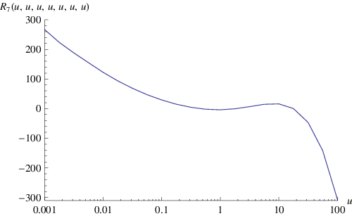
We have computed the remainder function for many other values of the cross-ratios. In Figure 11 we display the remainder function when all cross-ratios are equal.

7.2 Simple collinear limits

In this section we present numerical evidence that collinear limits of $n$ -gon Wilson loops with $n=7$ behave in the same way as the corresponding amplitude collinear limits. Collinear limits have been used very often as tools to check the consistency of ansatze for the expression of infinite sequences of scattering amplitudes, see for example [35]. In much the same way, by showing that Wilson loops, and in particular the remainder function, have the expected collinear limits, we can provide further evidence in support of the conjectured duality between the finite parts of these two a priori completely different quantities.

We begin with a brief review of the universal behaviour of scattering amplitudes under simple collinear limits. In this limit, one selects two adjacent momenta $p_{a}$ and $p_{b}$ , and sets

p_{a}\ =\ zP\ ,\qquad\qquad p_{b}\ =\ (1-z)P\ .

(7.3)

The collinear limit is taken by letting $P^{2}\to 0$ . Under this limit, scattering amplitudes behave in a well-known, universal way. Consider for instance a one-loop scattering amplitude, ${\cal A}_{n}^{1-{\rm loop}}$ . When the two momenta $p_{a}$ and $p_{b}$ become collinear, the amplitude is known to factorise as [35, 36, 37, 38]

	$\displaystyle{\cal A}_{n}^{1-{\rm loop}}(1,\ldots,a^{\lambda_{a}},b^{\lambda_{b}},\ldots,n)\;{\mathrel{\mathop{\kern 0.0pt\relbar\mskip-1.0mu\joinrel\longrightarrow}\limits^{a\parallel b}}}$		(7.4)
	$\displaystyle\hskip 28.45274pt\sum_{\sigma}\bigg[{\rm Split}^{\rm tree}_{-\sigma}(a^{\lambda_{a}},b^{\lambda_{b}})\ {\cal A}_{n-1}^{1-{\rm loop}}(1,\ldots,(a+b)^{\sigma},\ldots,n)$
	$\displaystyle\hskip 39.83368pt\ +\ {\rm Split}^{1-{\rm loop}}_{-\sigma}(a^{\lambda_{a}},b^{\lambda_{b}})\ {\cal A}_{n-1}^{\rm tree}(1,\ldots,(a+b)^{\sigma},\ldots,n)\bigg]\ .$

${\rm Split}^{\rm tree}$ are tree-level splitting amplitudes, whose explicit forms can be found, for instance, in [69]. ${\rm Split}^{1-{\rm loop}}$ is a one-loop splitting amplitude. Explicit formulae for this one-loop splitting amplitude, valid to all orders in the dimensional regularisation parameter $\epsilon$ , were presented in [70] and [71]. We quote here the result of [71] for the ${\cal N}=4$ theory:

{\rm Split}^{1-{\rm loop}}_{-\sigma}(a^{\lambda_{a}},b^{\lambda_{b}})\ =\ {\rm Split}^{\rm tree}_{-\sigma}(a^{\lambda_{a}},b^{\lambda_{b}})\ r_{S}^{(1)}(\epsilon;z,s_{ab})\ ,

(7.5)

where, to all orders in $\epsilon$ ,

r_{S}^{(1)}(\epsilon;z,s_{ab})\ :=\ {\hat{c}_{\Gamma}\over\epsilon^{2}}\Big({-s_{ab}\over\mu^{2}}\Big)^{-\epsilon}\left[1\,-\,\mbox{}_{2}F_{1}\left(1,-\epsilon,1-\epsilon,{z-1\over z}\right)\,-\,\mbox{}_{2}F_{1}\left(1,-\epsilon,1-\epsilon,{z\over z-1}\right)\right]\ ,

(7.6)

and $\hat{c}_{\Gamma}$ is defined in (3.11).

We now move on to consider the behaviour of the remainder function ${\cal R}_{n}$ as defined in (3.24) under collinear limits, following [21]. Consider then the two-loop term ${\cal M}^{(2)}_{n}(\epsilon)$ in the expansion of the amplitude, and write it as

{\cal M}^{(2)}_{n}(\epsilon)-{1\over 2}\Big({\cal M}^{(1)}_{n}(\epsilon)\Big)^{2}\ =\ f^{(2)}(\epsilon){\cal M}^{(1)}_{n}(2\epsilon)\,+\,C^{(2)}\,+\,{\cal R}_{n}\ \,+\,{\cal O}(\epsilon)\ ,

(7.7)

where $f^{(2)}(\epsilon):=f^{(2)}_{0}+f^{(2)}_{1}\epsilon+f^{(2)}_{2}\epsilon^{2}$ and $C^{(2)}$ are defined in (2.4), (2.5). Using (7.4) and (7.5), one sees that, under a simple collinear limit, the scalar function ${\cal M}^{(1)}$ must behave as [2]

	$\displaystyle{\cal M}^{(1)}_{n}$	$\displaystyle\to$	$\displaystyle{\cal M}^{(1)}_{n-1}+r_{S}^{(1)}(\epsilon;z,s_{ab})\ ,$		(7.8)
	$\displaystyle{\cal M}^{(2)}_{n}$	$\displaystyle\to$	$\displaystyle{\cal M}^{(2)}_{n-1}+r^{(1)}_{S}(\epsilon;z,s_{ab}){\cal M}^{(1)}_{n-1}+r_{S}^{(2)}(\epsilon;z,s_{ab})\ .$

It was shown in [1] that splitting amplitudes obey an iterative formula identical to the homogeneous form of the BDS conjecture for the amplitude, i.e.

r^{(2)}_{S}(\epsilon;z,s_{ab})-{1\over 2}\big(r^{(1)}(\epsilon;z,s_{ab})\big)^{2}\,=\,f^{(2)}(\epsilon)r_{S}^{(1)}(2\epsilon;z,s_{ab})\,+{\cal O}(\epsilon)\ .

(7.9)

Using (7.8) and (7.9), one sees that, under a simple collinear limit,

	$\displaystyle{\cal M}^{(2)}_{n}(\epsilon)$	$\displaystyle-{1\over 2}\Big({\cal M}^{(1)}_{n}(\epsilon)\Big)^{2}-f^{(2)}(\epsilon){\cal M}_{n}^{(1)}(2\epsilon)$
		$\displaystyle\rightarrow{\cal M}^{(2)}_{n-1}(\epsilon)-{1\over 2}\Big({\cal M}^{(1)}_{n-1}(\epsilon)\Big)^{2}-f^{(2)}(\epsilon){\cal M}_{n-1}^{(1)}(2\epsilon)\ .$		(7.10)

Equation (7.7) defined the finite remainder function ${\cal R}_{n}$ of the amplitude as

{\cal R}_{n}\ =\ {\cal M}^{(2)}_{n}(\epsilon)\,-\,{1\over 2}\Big({\cal M}^{(1)}_{n}(\epsilon)\Big)^{2}-f^{(2)}(\epsilon){\cal M}^{(1)}_{n}(2\epsilon)\,-\,C^{(2)}\,+{\cal O}(\epsilon)\ \ ,

(7.11)

and it follows from (7.10) that in the simple collinear limit ${\cal R}_{n}\ \to\ {\cal R}_{n-1}$ , as anticipated in (2.20).

What about simple collinear limits of Wilson loops? If the duality with amplitudes holds, we expect that the Wilson loop will have the same collinear limits as the amplitude, as discussed in (3.9).

Let us now specify this discussion to the seven-point Wilson loop case. Specifically, in the simple collinear limit of a seven-point amplitude one expects to find

{\cal R}_{7}^{\mathrm{WL}}\left(u_{14},u_{25},u_{36},u_{47},u_{15},u_{26},u_{37}\right)\rightarrow{\cal R}_{6}^{\mathrm{WL}}(u_{1},u_{2},u_{3})\ ,

(7.12)

where the seven-point basis of cross-ratios is defined in (7.1), while the six-point basis in (2.25). Notice that on the right hand side of (7.12) we do not allow for an additional constant term.

For concreteness we take $p_{6}$ and $p_{7}$ to be collinear. We set

p_{6}=x_{6}-x_{7}=zP\ ,\qquad p_{7}=x_{7}-x_{1}=(1-z)P\ ,

(7.13)

where as usual $P^{2}\to 0$ in the collinear limit. In this collinear limit, the cusp at $x_{7}$ is therefore “flattened”. This collinear limit of the seven-point kinematics is characterised by

	$\displaystyle x^{2}_{16}\to 0\ ,\qquad x^{2}_{27}=(1-z)x^{2}_{26}\ ,\qquad x^{2}_{57}=zx^{2}_{51}\ ,$		(7.14)
	$\displaystyle x^{2}_{37}=(1-z)x^{2}_{36}+zx^{2}_{13}\ ,\qquad x^{2}_{47}=(1-z)x^{2}_{46}+zx^{2}_{14}\ ,\$

with all other $x^{2}_{ij}$ segments unchanged.

As one can see in Figure 12, there are three cross-ratios which do not pass through the cusp at $x_{7}$ . The first two are members of our basis (7.1), whereas the third one is a product of members of our basis,

u_{14}:={x_{15}^{2}x_{34}^{2}\over x_{14}^{2}x_{35}^{2}}\ ,\qquad u_{25}:={x_{26}^{2}x_{35}^{2}\over x_{25}^{2}x_{36}^{2}}\ ,\qquad u_{36}\,u_{37}:={x_{13}^{2}x_{46}^{2}\over x_{14}^{2}x_{36}^{2}}\ .

(7.15)

These ratios agree precisely with the three variables of the six-point case,

u^{(7)}_{14}\rightarrow u^{(6)}_{14}=u_{2}\ ,\qquad u^{(7)}_{25}\rightarrow u^{(6)}_{25}=u_{3}\ ,\qquad u^{(7)}_{36}\,u^{(7)}_{37}\rightarrow u^{(6)}_{36}=u_{1}\ .

(7.16)

where the superscripts on the $u$ ’s denote the number of edges of the corresponding Wilson loop and $u_{1},u_{2},u_{3}$ are the six-point cross-ratios defined in [22] and given in (2.25). Specifically, the seven-point cross-ratios defined in (7.1) become (see (2.23))

	$\displaystyle u_{14}={x_{24}^{2}x_{15}^{2}\over x_{25}^{2}x_{14}^{2}}\ ,\quad u_{25}={x_{26}^{2}x_{35}^{2}\over x_{25}^{2}x_{36}^{2}}\ ,$
	$\displaystyle u_{36}={x_{46}^{2}\over x_{36}^{2}}{zx_{13}^{2}+(1-z)x_{36}^{2}\over zx_{14}^{2}+(1-z)x_{46}^{2}}\ ,\quad u_{47}={zx_{14}^{2}\over zx_{14}^{2}+(1-z)x_{46}^{2}}\ ,\quad u_{15}=0\ ,$
	$\displaystyle u_{26}={(1-z)x_{36}^{2}\over zx_{13}^{2}+(1-z)x_{36}^{2}}\ ,\quad u_{37}={x_{13}^{2}\over x_{14}^{2}}{zx_{14}^{2}+(1-z)x_{46}^{2}\over zx_{13}^{2}+(1-z)x_{36}^{2}}\ .$		(7.17)

As expected, it follows immediately that $u_{14}$ , $u_{25}$ and $u_{36}\,u_{37}$ are equal to the three cross-ratios of the six-point case, as dictated by (7.16). In addition, (7.17) imply that there are three constraints on the remaining four variables,

u_{15}=0\ ,\quad u_{47}+u_{26}\,u_{36}=1\ ,\quad u_{26}+u_{37}\,u_{47}=1\ .

(7.18)

Taking this into account, and solving the two constraints in (7.18) for $u_{47}$ and $u_{26}$ we conclude that the collinear limit relates the seven-point remainder function to the six-point one as follows:

	$\displaystyle{\cal R}_{7}^{\mathrm{WL}}(u_{14},u_{25},u_{36},u_{47},u_{15},u_{26},u_{37})$	$\displaystyle\rightarrow{\cal R}_{7}^{\mathrm{WL}}\left(u_{14},u_{25},u_{36},\frac{1-u_{36}}{1-u_{37}u_{36}},0,\frac{1-u_{37}}{1-u_{37}u_{36}},u_{37}\right)$
		$\displaystyle={\cal R}_{6}^{\mathrm{WL}}(u_{37}u_{36},u_{14},u_{25})\ .$		(7.19)

Note that three of the seven variables on the left hand side of (7.19) are constrained, leaving four variables free. Since the right hand side is a function of only three variables, it follows that the left hand side actually does not depend on one combination: $u_{37}/u_{36}:=\kappa$ . Thus we can rewrite (7.19) in terms of the six-point cross-ratios $u_{i}$ and $\kappa$ as

{\cal R}_{7}^{\mathrm{WL}}\left(u_{2},u_{3},\sqrt{u_{1}/\kappa},\frac{1-\sqrt{u_{1}/\kappa}}{1-u_{1}},0,\frac{1-\sqrt{u_{1}\kappa}}{1-u_{1}},\sqrt{u_{1}\kappa}\right)={\cal R}_{6}^{\mathrm{WL}}(u_{1},u_{2},u_{3})\ ,

(7.20)

and note that the left hand side must therefore be independent of the variable $\kappa$ . This can be thought of as the $z$ -independence of ${\cal R}_{7}^{\mathrm{WL}}$ in the collinear limit – which is precisely the feature one would expect from the scattering amplitude.

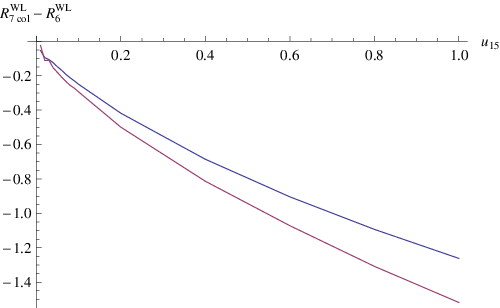
We have computed ${\cal R}_{7}^{\mathrm{WL}}$ in the collinear limit and have confirmed that (7.20) does hold within the errors and that no dependence on $\kappa$ is found (see Table 3 and Figure 13 for example). Again, we stress the absence on the right hand side of (7.20) of any additional constant term.

$(u_{1},u_{2},u_{3})$	${\cal R}^{\mathrm{WL}}_{7\mathrm{col}}(\kappa=2.5)$	${\cal R}^{\mathrm{WL}}_{7\mathrm{col}}(\kappa=4.9)$	${\cal R}^{\mathrm{WL}}_{6}$
$(1/10,1,1)$	-2.78972	-2.76053	-2.73441

Table 3: Checks of the collinear limit

{\cal R}^{\mathrm{WL}}_{7}\rightarrow{\cal R}^{\mathrm{WL}}_{6}

. We present

{\cal R}^{\mathrm{WL}}_{7\rm{col}}(\kappa):={\cal R}_{7}^{\mathrm{WL}}\big(u_{2},u_{3},\sqrt{u_{1}/\kappa},\frac{1-\sqrt{u_{1}/\kappa}}{1-u_{1}},0.01,\frac{1-\sqrt{u_{1}\kappa}}{1-u_{1}},\sqrt{u_{1}\kappa}\big)

for different values of

\kappa

, together with its collinear limit

{\cal R}_{6}(u_{1},u_{2},u_{3})

for

(u_{1},u_{2},u_{3})=(1/10,1,1)

. Within numerical errors the values agree.

In the following section we compare these results with what can be learned from the multi-collinear limits.

7.3 Multi-collinear limits

Here we would like to derive the multi-collinear equivalent of the general reduction formulae in (3.9), (7.19)-(7.20) for $n$ -gon Wilson loops.

The first non-trivial case is a triple collinear limit of a six-point configuration considered in Section 5 of [21]. In the limit where $p_{4}$ , $p_{5}$ and $p_{6}$ become collinear one has

p_{4}:=x_{4}-x_{5}=z_{1}P\ ,\quad p_{5}=x_{5}-x_{6}=z_{2}P\ ,\quad p_{6}=x_{6}-x_{1}=z_{3}P\ ,\quad z_{1}+z_{2}+z_{3}=1\ .

(7.21)

In this limit, the two-loop scalar function ${\cal M}^{(2)}_{6}$ behaves as [21]

{\cal M}^{(2)}_{6}\to{\cal M}_{4}^{(2)}\,+\,{\cal M}_{4}^{(1)}\,r_{S}^{(1)}\Big({s_{45}\over s_{456}},{s_{56}\over s_{456}},z_{1},z_{3},\epsilon\Big)\,+\,r_{S}^{(2)}\Big({s_{45}\over s_{456}},{s_{56}\over s_{456}},z_{1},z_{3},\epsilon\Big)\ ,

(7.22)

where $r_{S}^{(1)}$ and $r_{S}^{(2)}$ are the one- and two-loop triple splitting amplitudes. The two-loop triple splitting amplitude does not satisfy an iteration relation similar to the that found in [1] for the simple splitting amplitude (7.9) [21]. It can however be decomposed into a term with does, plus a two-loop finite remainder, as

r_{S}^{(2)}\ :=\ r_{S}^{(2)\,\mathrm{BDS}}\,+\,\widetilde{{\cal R}}\ .

(7.23)

It was shown in [21] that $\widetilde{{\cal R}}$ is nothing but the finite remainder function at six points evaluated in the triple collinear kinematics. Indeed, in the triple collinear limit the six-point cross-ratios remain independent and do not vanish, $u_{i}\to\bar{u}_{i}$ , $i=1,2,3$ , where

\bar{u}_{1}={1\over 1-z_{3}}{s_{45}\over s_{456}}\ ,\quad\bar{u}_{2}={1\over 1-z_{1}}{s_{56}\over s_{456}}\ ,\quad\bar{u}_{3}={z_{1}z_{3}\over(1-z_{1})(1-z_{3})}\ .

(7.24)

Hence,

{\cal R}_{6}(u_{1},u_{2},u_{3})\to{\cal R}_{6}(\bar{u}_{1},\bar{u}_{2},\bar{u}_{3})\ .

(7.25)

If we now take the triple collinear limit of the remainder function as defined from (7.11), and use (7.22) and (7.23), we get

{\cal R}_{6}(u_{1},u_{2},u_{3})\ \to\ {\cal R}_{4}\,+\,\widetilde{{\cal R}}(\bar{u}_{1},\bar{u}_{2},\bar{u}_{3})\ .

(7.26)

Using that ${\cal R}_{4}=0$ , and comparing (7.26) to (7.25) we get at once that

\widetilde{{\cal R}}(\bar{u}_{1},\bar{u}_{2},\bar{u}_{3})\ =\ {\cal R}_{6}(\bar{u}_{1},\bar{u}_{2},\bar{u}_{3})\ .

(7.27)

Assuming further dual conformal invariance, the conclusion of [21] is that determining the remainder function ${\cal R}_{6}$ in the triple collinear limit is equivalent to determining it in full generality.

We can now derive the triple collinear limit of the two-loop $n$ -point remainder function for general $n\geq 6$ . Using (7.27) we have

{\cal R}_{n}\ \to\ {\cal R}_{n-2}\,+\,{\cal R}_{6}(\bar{u}_{1},\bar{u}_{2},\bar{u}_{3})\ ,

(7.28)

where $(\bar{u}_{1},\bar{u}_{2},\bar{u}_{3})$ are still defined by (7.24) (in the case where the collinear momenta are $p_{4}$ , $p_{5}$ and $p_{6}$ ).

What about Wilson loops? Similarly to our discussion of simple collinear limits, we expect that, for Wilson loops, the triple collinear limit of the Wilson loop remainder function is given by

{\cal R}_{n}^{\mathrm{WL}}\left(u_{14},u_{25},u_{36},u_{47},u_{15},u_{26},u_{37}\right)\ \rightarrow\ {\cal R}_{n-2}^{\mathrm{WL}}\,+\,{\cal R}_{6}^{\mathrm{WL}}(\bar{u}_{1},\bar{u}_{2},\bar{u}_{3})\ .

(7.29)

Now consider a triple collinear limit of a heptagon Wilson loop, where $p_{5}$ , $p_{6}$ and $p_{7}$ are collinear,

p_{5}=x_{5}-x_{6}=z_{1}P\ ,\quad p_{6}=x_{6}-x_{7}=z_{2}P\ ,\quad p_{7}=x_{7}-x_{1}=z_{3}P\ ,\quad z_{1}+z_{2}+z_{3}=1\ .

(7.30)

In this limit,

{\cal R}_{7}^{\mathrm{WL}}\ \to\ {\cal R}_{6}^{\mathrm{WL}}(\bar{u}_{1},\bar{u}_{2},\bar{u}_{3})\ ,

(7.31)

since there is no five-point remainder function.

For our present case of collinear $p_{5}$ , $p_{6}$ and $p_{7}$ the variables $\bar{u}_{i}$ read

\bar{u}_{1}={1\over 1-z_{3}}{x_{57}^{2}\over x_{15}^{2}}\ ,\quad\bar{u}_{2}={1\over 1-z_{1}}{x_{16}^{2}\over x_{15}^{2}}\ ,\quad\bar{u}_{3}={z_{1}z_{3}\over(1-z_{1})(1-z_{3})}\ .

(7.32)

The triple collinear limit (7.30) of the seven-point kinematics gives

	$\displaystyle x^{2}_{15}\sim x^{2}_{16}\sim x^{2}_{57}\to 0\ ,$
	$\displaystyle x^{2}_{27}=z_{3}x^{2}_{25}\ ,\quad x^{2}_{26}=(1-z_{1})x^{2}_{25}\ ,\quad x^{2}_{46}=z_{1}x^{2}_{41}\ ,\quad x^{2}_{47}=(1-z_{3})x^{2}_{41}\ ,$
	$\displaystyle x^{2}_{36}=(1-z_{1})x^{2}_{35}+z_{1}x^{2}_{13}\ ,\quad x^{2}_{37}=(1-z_{3})x^{2}_{13}+z_{3}x^{2}_{35}\ ,$		(7.33)

with all other $x^{2}_{ij}$ segments unmodified. The cross-ratios $u_{ij}$ take the form:

	$\displaystyle u_{14}=0\ ,\quad u_{25}={(1-z_{1})x_{35}^{2}\over z_{1}x_{13}^{2}+(1-z_{1})x_{35}^{2}}$
	$\displaystyle u_{36}={z_{1}\over 1-z_{3}}{z_{3}x_{35}^{2}+(1-z_{3})x_{13}^{2}\over z_{1}x_{13}^{2}+(1-z_{1})x_{35}^{2}}\ ,\quad u_{47}={1\over 1-z_{3}}{x_{57}^{2}\over x_{15}^{2}}\ ,\quad u_{15}={1\over 1-z_{1}}{x_{16}^{2}\over x_{15}^{2}}\ ,$
	$\displaystyle u_{26}={z_{3}\over 1-z_{1}}{z_{1}x_{13}^{2}+(1-z_{1})x_{35}^{2}\over z_{3}x_{35}^{2}+(1-z_{3})x_{13}^{2}}\ ,\quad u_{37}={(1-z_{3})x_{13}^{2}\over z_{3}x_{35}^{2}+(1-z_{3})x_{13}^{2}}\ .$		(7.34)

These relations imply two things. First we note that there are three constraints on the seven variables,

u_{14}=0\ ,\quad u_{25}+u_{36}u_{37}=1\ ,\quad u_{37}+u_{25}u_{26}=1\ ,

(7.35)

leaving four variables unconstrained, out of which the three conformal ratios coincide with the $\bar{u}_{i}$ variables of (7.32),

u_{47}=\bar{u}_{1}\ ,\quad u_{15}=\bar{u}_{2}\ ,\quad u_{26}u_{36}=\bar{u}_{3}\ .

(7.36)

Taking this into account, and solving the two constraints in (7.35) for $u_{14}$ and $u_{35}$ we conclude that the triple collinear limit relates the seven-point remainder function to the six-point one as follows:

{\cal R}_{7}^{\mathrm{WL}}\left(0,\frac{1-u_{36}}{1-u_{26}u_{36}},u_{36},u_{47},u_{15},u_{26},\frac{1-u_{26}}{1-u_{36}u_{26}}\right)=\,{\cal R}_{6}^{\mathrm{WL}}(u_{47},u_{15},u_{26}u_{36})\ .

(7.37)

Notice that since ${\cal R}_{7}^{\mathrm{WL}}$ is invariant under cyclic interchange of its variables, this is exactly the same equation as we had before in the simple collinear limit (7.19) (alas expressed in terms of $u_{36}$ , $u_{47}$ , $u_{15}$ and $u_{26}$ ).

We conclude that the simple and the triple collinear limits described by (7.19) and (7.37) give identical information about ${\cal R}_{7}^{\mathrm{WL}}$ . As before, the left hand side of (7.37) cannot depend on one particular combination of cross-ratios, namely $u_{36}/u_{26}:=\kappa$ . Thus, we can rewrite (7.37) as

{\cal R}_{7}^{\mathrm{WL}}\left(0,\frac{1-\sqrt{\bar{u}_{3}\kappa}}{1-\bar{u}_{3}},\sqrt{\bar{u}_{3}\kappa},\bar{u}_{1},\bar{u}_{2},\sqrt{\bar{u}_{3}/\kappa},\frac{1-\sqrt{\bar{u}_{3}/\kappa}}{1-\bar{u}_{3}}\right)=\,{\cal R}_{6}^{\mathrm{WL}}(\bar{u}_{1},\bar{u}_{2},\bar{u}_{3})\ ,

(7.38)

and note that the left hand side must be independent of the variable $\kappa$ .

Finally, we have investigated the quadruple collinear limit, which is the highest non-trivial multi-collinear limit one can take on the seven-point kinematics. We have found in this limit that all seven cross-ratios are (a) mutually independent, and (b) are expressed entirely in terms of the multi-collinear kinematics (i.e. they are functions of $z_{1},\ldots,z_{4}$ and ratios of kinematic invariants involving only the collinear momenta). In this way, the quadruple collinear limit does not add any non-trivial functional constraints on the ${\cal R}_{7}$ , however, it elucidates its physical (scattering amplitudes-based) meaning,

{\cal R}_{7}^{\mathrm{WL}}(u_{14},u_{25},u_{36},u_{47},u_{15},u_{26},u_{37})\,\,=\,\Delta{\rm split}_{4}:=\,r_{S4}^{(2)}-r_{S4}^{(2)\,{\rm BDS}}\ ,

(7.39)

where $\Delta{\rm split}_{4}$ is the normalised two-loop level part of the quadruple splitting function $r_{S4}^{(2)}$ which is not already accounted by the BDS contribution $r_{S4}^{(2)\,{\rm BDS}}$ . Hence, similarly to the six-point case discussed in previously [21], we see that the remainder function ${\cal R}_{7}$ is entirely determined by the quadruple splitting function.

8 Eight-point Wilson loops and beyond

It is natural to seek beyond the encouraging results at seven points given above, and see if these persist at eight points. The discussion earlier indicates that there are twelve independent conformal cross-ratios in this case (we take the external momenta to be on shell and do not impose the Gram determinant constraint), whereas there are twenty independent momentum invariants. These independent invariants may be taken to be

x^{2}_{i\;i+2},x^{2}_{i+4\;i+6},\;x^{2}_{i\;i+3},\;x^{2}_{i+4\;i+7},\;x^{2}_{i\;i+4}\ ,\quad{i=1,\ldots,4}\ .

(8.1)

We will use the following twelve cross-ratios:

u_{i\;i+3}\ ,\quad i=1,\ldots,8\ ,\qquad u_{i\;i+4}\ ,\quad i=1,\ldots,4\ ,

(8.2)

and label these $u_{1},...,u_{12}$ . Instead of the twenty momentum invariants given in (8.1), we will use these twelve cross-ratios, plus the following eight momentum invariants

x^{2}_{i+5\;i+8},\;x^{2}_{i\;i+4}\ ,\quad i=1,\dots,4\ ,

(8.3)

which we will call $m_{1},\dots,m_{8}$ . The remaining momentum invariants $x^{2}_{i\;i+2},x^{2}_{i+4\;i+6}$ and $x^{2}_{i+1\;i+4}$ , for $i=1,\dots,4$ , are then dependent variables.

The first question to study is whether the eight-point Wilson loop remainder function ${\cal R}_{8}^{\mathrm{WL}}$ is only a function of the twelve conformal cross-ratios (8.2), and not of the additional eight invariants (8.3). To do this, one may fix a choice of the cross-ratios, then calculate the eight-point remainder function for various choices of kinematics, corresponding to different choices of the variables (8.3). For example, in Table 4 we have listed some numerical results for the case of all the cross-ratios of (8.2) equal to one. We find similar results for more generic values of the cross-ratios – an example is given in Table 5.

$(m_{1},\dots,m_{8})$	${\cal R}_{8}^{\mathrm{WL}}$
$(-1,-1,-1,-1,-1,-1,-1,-1)$	-4.603
$(-2,-2,-2,-2,-2,-2,-2,-2)$	-4.602
$(-1,-2,-4,-8,-1,-2,-4,-8)$	-4.605
$(-5,-3,-5,-3,-1,-3,-5,-7)$	-4.605

Table 4: The remainder function

{\cal R}_{8}^{\mathrm{WL}}

for

u_{1}=u_{2}=\dots=u_{12}=1

and different choices of the other independent invariants (8.3). The errors in

{\cal R}_{8}^{\mathrm{WL}}

are approximately

0.02

$(m_{1},\dots,m_{8})$	${\cal R}_{8}^{\mathrm{WL}}$
$(-2,-3,-4,-1,-5,-6,-7,-8)$	5.993
$(-1/3,-1/4,-1/9,-1/2,-1/8,-1/7,-1/6,-1)$	5.984

Table 5: The remainder function

{\cal R}_{8}^{\mathrm{WL}}

for the choice of cross-ratios

(u_{1},\dots,u_{12})=(2,3,4,1/2,1/3,1/4,1/5,1,1/5,1/6,1/7,1/8)

and two choices of the other independent invariants (8.3). The errors in

{\cal R}_{8}^{\mathrm{WL}}

are approximately

0.04

These results support the conjecture that the eight-point remainder function ${\cal R}_{8}^{\mathrm{WL}}$ is a function of the twelve cross-ratios (8.2) alone, and not of any other independent additional momentum invariants.

Given this, a second question concerns symmetries of the function ${\cal R}_{8}^{\mathrm{WL}}(u_{1},...,u_{12})$ . The Wilson loop is invariant under cyclic permutations of the external momenta as well as under parity. For the case of eight points, this implies that the remainder function ${\cal R}_{8}^{\mathrm{WL}}(u_{1},...,u_{12})$ should be invariant under cyclic permutations of the first eight and last four cross-ratios simultaneously, as well as being invariant under the simultaneous reversal of both the first eight and last four cross-ratios. We find numerical agreement with this – for example,

	$\displaystyle{\cal R}_{8}^{\mathrm{WL}}(2,2,1,1,1,1,1,1,1,1,1,1)=-3.712,$
	$\displaystyle{\cal R}_{8}^{\mathrm{WL}}(1,2,2,1,1,1,1,1,1,1,1,1)=-3.712,$		(8.4)

with errors $\sim 0.02$ . We have also seen numerically in a number of cases that there is no invariance under more general permutations of the cross-ratios.

Let us now consider collinear limits of the eight-point remainder function. As an example we take $p_{7}$ and $p_{8}$ to be collinear. We set

p_{7}=x_{7}-x_{8}=zP\ ,\qquad p_{8}=x_{8}-x_{1}=(1-z)P\ ,

(8.5)

where as usual $P^{2}\to 0$ in the collinear limit. In this collinear limit, the cusp at $x_{8}$ is “flattened”. In this limit we find that the eight-point cross-ratios $(u_{14},u_{25},u_{36},u_{15},u_{26})$ reduce directly to the cross-ratios in the seven-point case with the same names, $u_{16}\rightarrow 0$ and the seven-point cross-ratios $(u_{47},u_{37})$ are given in terms of the eight-point ones as $(u_{47}u_{48},u_{37}u_{38})$ respectively. Finally, we have the following relations amongst the eight-point cross-ratios:

	$\displaystyle u_{27}u_{37}u_{38}=-1+u_{27}+u_{38},$
	$\displaystyle(-1+u_{27}+u_{38})u_{47}=u_{38}(1-u_{58}),$
	$\displaystyle u_{48}u_{58}=1-u_{27}u_{37},$
	$\displaystyle u_{37}(-u_{38}-u_{47}+u_{38}u_{47}+u_{38}u_{58})=-1+u_{58},$		(8.6)

which are solved by

	$\displaystyle u_{27}=\frac{-1+u_{38}}{-1+u_{37}u_{38}},$
	$\displaystyle u_{58}=\frac{-1+u_{37}u_{38}+u_{37}u_{47}-u_{37}u_{38}u_{47}}{-1+u_{37}u_{38}},$
	$\displaystyle u_{48}=\frac{-1+u_{37}}{-1+u_{37}u_{38}+u_{37}u_{47}-u_{37}u_{38}u_{47}}.$		(8.7)

The three variables $(u_{37},u_{38},u_{47})$ in the above are then freely specifiable.

Analysis of the remainder function given earlier implies that in the collinear limit

{\cal R}_{8}^{\mathrm{WL}}\rightarrow{\cal R}_{7}^{\mathrm{WL}}\ .

(8.8)

Hence in the collinear limit (8.5) one should have

	$\displaystyle{\cal R}_{8}^{\mathrm{WL}}(u_{14},u_{25},u_{36},u_{47},u_{58},u_{16},u_{27},u_{38},u_{15},u_{26},u_{37},u_{48})\rightarrow$
	$\displaystyle{\cal R}_{8}^{\mathrm{WL}}\left(u_{14},u_{25},u_{36},u_{47},u_{58}^{},0,u_{27}^{},u_{38},u_{15},u_{26},u_{37},u_{48}^{*}\right)$
	$\displaystyle={\cal R}_{7}^{\mathrm{WL}}(u_{14},u_{25},u_{36},u_{47}u_{48}^{*},u_{15},u_{26},u_{37}u_{38})\ ,$		(8.9)

where the stars in the above indicate that the solutions (8.7) are to be inserted.

One can test this directly. For example, for the choices of values for the independently specifiable eight-point cross-ratio variables

(u_{14},u_{25},u_{36},u_{47},u_{83},u_{15},u_{26},u_{37})=(1,1,1,1,1/2,1,1,1/2),

(8.10)

and taking $u_{61}=0.001$ one finds

	$\displaystyle{\cal R}_{8}^{\mathrm{WL}}(u_{14},u_{25},u_{36},u_{47},u_{58}^{},0.001,u_{72}^{},u_{83},u_{15},u_{26},u_{37},u_{48}^{*})=-4.2756,$
	$\displaystyle{\cal R}_{7}^{\mathrm{WL}}(u_{14},u_{25},u_{36},u_{47}u_{48},u_{15},u_{26},u_{37}u_{38})=-4.2906\ ,$		(8.11)

with errors of $0.147$ and $0.005$ respectively.

The success of the above numerical tests of the conformal symmetry, functional symmetries and collinear limits of the eight-point remainder function supports the conjecture that the Wilson loop is correctly reproducing the physical amplitude at this level.

There are no further conceptual or computational obstacles to generalising the above work beyond eight-point Wilson loops, apart from the question of the computer time required to numerically calculate the integrals – we stress that no new integrals arise in the Wilson loop approach to $n$ -point two-loop diagrams for any $n$ , apart from those which we have already discussed, and we are able to calculate all the diagrams introduced for generic values of the momentum variables $Q_{i}$ (numerically, and in a number of cases, analytically).

This means that we have full numerical control over two-loop $n$ -gon Wilson loops and, if the correspondence with amplitudes continues to hold, over $n$ -point MHV amplitudes at arbitrary $n$ in the planar ${\cal N}=4$ theory. This should be contrasted with the situation where one calculates amplitudes directly.

Acknowledgements

It is a pleasure to thank Mert Aybat, Zvi Bern, Lance Dixon, James Drummond, George Georgiou, Nigel Glover, David Kosower, Lorenzo Magnea and Marcus Spradlin for discussions, and especially Lance Dixon for useful comments and Radu Roiban for discussions and initial collaboration on this project. PH, VVK and GT would also like to thank the ETH Zürich for hospitality and support during the earlier stage of this project. This work was supported by the Swiss National Science Foundation under contract 200021-117873, and by the STFC under the Queen Mary Rolling Grant ST/G000565/1 and the IPPP Grant ST/G000905/1. The work of PH is supported by an EPSRC Standard Research Grant EP/C544250/1. VVK acknowledges a Leverhulme Research Fellowship and GT is supported by an EPSRC Advanced Research Fellowship EP/C544242/1 and by an EPSRC Standard Research Grant EP/C544250/1.

A A note on conventions

Wilson loops are computed in dimensional reduction in $D=4-2{\epsilon_{\rm\mbox{\tiny UV}}}$ dimensions with ${\epsilon_{\rm\mbox{\tiny UV}}}>0$ to regularise the UV divergences. To facilitate the comparison with scattering amplitudes (which require infrared regularisation) we introduce

\epsilon=-{\epsilon_{\rm\mbox{\tiny UV}}}\ .

(A.1)

The perturbative expansion of the Wilson loop is characterised by (3.2), (3.3):

	$\displaystyle\langle W[{\cal C}_{n}]\rangle$	$\displaystyle=$	$\displaystyle 1\,+\,\sum_{l=1}^{\infty}a^{l}W^{(l)}_{n}\ =\ \exp\sum_{l=1}^{\infty}a^{l}w^{(l)}_{n}\ ,$		(A.2)
	$\displaystyle w^{(2)}_{n}$	$\displaystyle=$	$\displaystyle W^{(2)}_{n}\,-\,{1\over 2}\,(W^{(1)}_{n})^{2}\ ,$		(A.3)

and (3.21) defines the Laurent expansion in $\epsilon$ for the two-loop contribution,

w^{(2)}_{n}\ =\ \sum_{i=1}^{n}{\left(-{x_{ii+2}^{2}\over\mu^{2}}\right)^{-2\epsilon}}\Big({w^{(2)}_{-2}\over\epsilon^{2}}+{w^{(2)}_{-1}\over\epsilon}\Big)\ +\ F^{(2)}_{n}\,+\,{\cal O}(\epsilon)\ ,

(A.4)

where $F^{(2)}_{n}$ is the finite part of the Wilson loop.

In [23] the exponent of the Wilson loop in (A.2) was defined as $aw^{(1)}+2a^{2}w^{(2)}+\cdots$ , and thus a corresponding factor of $1/2$ would need to be introduced in front of the right hand side in (A.3) and in (A.4) if we were to switch to their conventions. Therefore our singular terms $w_{-2}$ , $w_{-1}$ and the finite part $F^{(2)}_{n}$ in (A.4) are related to the $A_{-2}$ , $A_{-1}$ and $A_{0}$ contributions of [25] as follows:

w_{-2}=\sum_{\alpha}A_{-2}^{(\alpha)}\ ,\qquad w_{-1}=-\sum_{\alpha}A_{-1}^{(\alpha)}\ ,\qquad F^{(2)}_{n}=2\sum_{\alpha}A_{0}^{(\alpha)}\ .

(A.5)

The minus sign in the second equation is due to (A.1).

B Most general hard diagram

Below is the result for the diagram where a three-point vertex is attached to three lightlike momenta $p_{1}$ , $p_{2}$ , $p_{3}$ of the Wilson loop, which we call the “hard diagram” as it is the most difficult to evaluate analytically in general. These momenta are separated by the three, not necessarily lightlike momenta, $Q_{3}$ , $Q_{1}$ , $Q_{2}$ , where $Q_{3}$ is between $p_{1}$ and $p_{2}$ and so on (see Figure 2). Momentum conservation is then $\sum_{i=1}^{3}(p_{i}+Q_{i})=0$ . We also set $D=4-2{\epsilon_{\rm\mbox{\tiny UV}}}=4+2\epsilon$ where ${\epsilon_{\rm\mbox{\tiny UV}}}=-\epsilon>0$ . The special four-point case is considered later.

We write this diagram in the most general configuration as⁹⁹ 9 We remind the reader that we will always suppress the common prefactor defined in (4.1) from the expression of all diagrams.

		$\displaystyle f_{H}(p_{1},p_{2},p_{3};Q_{1},Q_{2},Q_{3})$
		$\displaystyle:={1\over 8}\,{\Gamma(2-2{\epsilon_{\rm\mbox{\tiny UV}}})\over\Gamma(1-{\epsilon_{\rm\mbox{\tiny UV}}})^{2}}\int_{0}^{1}\!\Big(\prod_{i=1}^{3}d\tau_{i}\Big)\int_{0}^{1}\!\Big(\prod_{i=1}^{3}\,d\alpha_{i}\Big)\delta(1-\sum_{i=1}^{3}\alpha_{i})\ (\alpha_{1}\alpha_{2}\alpha_{3})^{-{\epsilon_{\rm\mbox{\tiny UV}}}}{\mathcal{N}\over\mathcal{D}^{2-2{\epsilon_{\rm\mbox{\tiny UV}}}}}\ ,$		(B.1)

where

\mathcal{D}:=-\alpha_{1}\alpha_{2}(z_{1}-z_{2})^{2}-\alpha_{2}\alpha_{3}(z_{2}-z_{3})^{2}-\alpha_{1}\alpha_{3}(z_{1}-z_{3})^{2}\ ,

(B.2)

and

$\displaystyle(z_{1}-z_{2})^{2}$	$\displaystyle=$	$\displaystyle Q_{3}^{2}+2(p_{1}p_{2})(1-\tau_{1})\tau_{2}+2(Q_{3}p_{1})(1-\tau_{1})+2(Q_{3}p_{2})\tau_{2}\ ,$	(B.3)
$\displaystyle(z_{2}-z_{3})^{2}$	$\displaystyle=$	$\displaystyle Q_{1}^{2}+2(p_{2}p_{3})(1-\tau_{2})\tau_{3}+2(Q_{1}p_{2})(1-\tau_{2})+2(Q_{1}p_{3})\tau_{3}\ ,$
$\displaystyle(z_{3}-z_{1})^{2}$	$\displaystyle=$	$\displaystyle Q_{2}^{2}+2(p_{3}p_{1})(1-\tau_{3})\tau_{1}+2(Q_{2}p_{3})(1-\tau_{3})+2(Q_{2}p_{1})\tau_{1}\ .$

The original expressions for the $z_{i}-z_{i+1}$ are

\displaystyle z_{i}-z_{i+1}

\displaystyle=

\displaystyle Q_{i+2}+p_{i}(1-\tau_{i})+p_{i+1}\tau_{i+1}\ ,\qquad i=1,2,3\ .

(B.4)

The expression for the numerator ${\cal N}$ has two kinds of terms. The first three lines involve $\tau$ and $\alpha$ parameters, whereas the remaining three lines involve only the $\tau$ parameters. It is given by

$\displaystyle{\cal N}$	$\displaystyle=$	$\displaystyle 2(p_{1}p_{2})(p_{1}p_{3})\Big[\alpha_{1}\alpha_{2}(1-\tau_{1})+\alpha_{3}\alpha_{1}\tau_{1}\Big]$	(B.5)
	$\displaystyle+$	$\displaystyle 2(p_{1}p_{2})(p_{2}p_{3})\Big[\alpha_{2}\alpha_{3}(1-\tau_{2})+\alpha_{1}\alpha_{2}\tau_{2}\Big]$	(B.6)
	$\displaystyle+$	$\displaystyle 2(p_{1}p_{3})(p_{2}p_{3})\Big[\alpha_{3}\alpha_{1}(1-\tau_{3})+\alpha_{2}\alpha_{3}\tau_{3}\Big]$	(B.7)
	$\displaystyle+$	$\displaystyle 2\alpha_{1}\alpha_{2}\Big[2(p_{1}p_{2})(p_{3}Q_{3})-(p_{2}p_{3})(p_{1}Q_{3})-(p_{3}p_{1})(p_{2}Q_{3})\Big]$	(B.8)
	$\displaystyle+$	$\displaystyle 2\alpha_{2}\alpha_{3}\Big[2(p_{2}p_{3})(p_{1}Q_{1})-(p_{3}p_{1})(p_{2}Q_{1})-(p_{1}p_{2})(p_{3}Q_{1})\Big]$	(B.9)
	$\displaystyle+$	$\displaystyle 2\alpha_{3}\alpha_{1}\Big[2(p_{3}p_{1})(p_{2}Q_{2})-(p_{1}p_{2})(p_{3}Q_{2})-(p_{2}p_{3})(p_{1}Q_{2})\Big]\ .$	(B.10)

B.1 Four-point case

The four-point case can be obtained by setting

Q_{3}=Q_{1}=0\ ,\qquad Q_{2}=p_{4}=-(p_{1}+p_{2}+p_{3})\ ,

(B.11)

where now $Q_{2}^{2}=p_{4}^{2}=0$ . The expression for ${\cal N}$ in (B.5) then simplifies to

$\displaystyle{\cal N}$	$\displaystyle=$	$\displaystyle 2(p_{1}p_{2})(p_{1}p_{3})\,(1-\tau_{1})\alpha_{1}(\alpha_{2}-\alpha_{3})$	(B.12)
	$\displaystyle+$	$\displaystyle 2(p_{1}p_{2})(p_{2}p_{3})\Big[\alpha_{2}\alpha_{3}(1-\tau_{2})+\alpha_{1}(2\alpha_{3}+\alpha_{2}\tau_{2})\Big]$	(B.13)
	$\displaystyle+$	$\displaystyle 2(p_{1}p_{3})(p_{2}p_{3})\,\tau_{3}\alpha_{3}(\alpha_{2}-\alpha_{1})\ .$	(B.14)

In this special case we have

$\displaystyle(z_{1}-z_{2})^{2}$	$\displaystyle=$	$\displaystyle 2(p_{1}p_{2})(1-\tau_{1})\tau_{2}\ ,$	(B.15)
$\displaystyle(z_{2}-z_{3})^{2}$	$\displaystyle=$	$\displaystyle 2(p_{2}p_{3})(1-\tau_{2})\tau_{3}\ ,$
$\displaystyle(z_{3}-z_{1})^{2}$	$\displaystyle=$	$\displaystyle 2(p_{3}p_{1})(1-\tau_{3})\tau_{1}+2(p_{3}p_{4})(1-\tau_{3})+2(p_{1}p_{4})\tau_{1}\ ,$

where we can set

$\displaystyle s$	$\displaystyle:=$	$\displaystyle 2(p_{1}p_{2})=2(p_{3}p_{4})\ ,$	(B.16)
$\displaystyle t$	$\displaystyle:=$	$\displaystyle 2(p_{2}p_{3})=2(p_{1}p_{4})\ ,$	(B.17)
$\displaystyle u$	$\displaystyle:=$	$\displaystyle 2(p_{1}p_{3})=2(p_{2}p_{4})\ ,$	(B.18)

and $s+t+u=0$ .

The denominator in the four-point case then simplifies to

{\cal D}:=s\,\alpha_{1}\alpha_{2}\tau_{2}(1-\tau_{1})+t\,\alpha_{2}\alpha_{3}\tau_{3}(1-\tau_{2})+\alpha_{3}\alpha_{1}\Big[s(1-\tau_{1})(1-\tau_{3})+t\tau_{1}\tau_{3}\Big]\ .

(B.19)

Notice that in the six-point case there is a new diagram where all the $Q_{i}$ ’s are made of a single lightlike momentum; in this diagram $Q_{1}^{2}=Q_{2}^{2}=Q_{3}^{2}=0$ . One should find that the result for the corresponding integral ${\cal I}$ is finite in four dimensions.

C Curtain diagram

We call “curtain” diagrams those diagrams where two propagators connect three different edges, as depicted in Figure 3. We use the same notation as in the three-point vertex case above, with propagators stretching from $p_{1}$ to $p_{2}$ (with end-points $z_{1}(\sigma_{1})$ and $z_{2}(\tau_{2})$ ) and from $p_{1}$ to $p_{3}$ (with end-points $z_{1}(\tau_{1})$ and $z_{3}(\tau_{3})$ ).

Just from looking at the diagram we should have the following symmetry: $p_{2}\leftrightarrow p_{3}$ $Q_{2}\leftrightarrow Q_{3}$ . We have

$\displaystyle z_{1}(\tau_{1})$	$\displaystyle=p_{1}\tau_{1}$	(C.1)
$\displaystyle z_{1}(\sigma_{1})$	$\displaystyle=p_{1}\sigma_{1}$	(C.2)
$\displaystyle z_{2}(\tau_{2})$	$\displaystyle=p_{2}\tau_{2}+p_{1}+Q_{3}$	(C.3)
$\displaystyle z_{3}(\tau_{3})$	$\displaystyle=-p_{3}\tau_{3}-Q_{2}\ .$	(C.4)

The exponentiation theorem says we should only consider the diagram where the internal gluon propagators cross - this gives the constraint $\tau_{1}>\sigma_{1}$ .

The diagram represents the following contribution to the Wilson loop:

-{1\over 2}\int_{0}^{1}\!\Big(\prod_{i=1}^{3}d\tau_{i}\Big)\,\int_{0}^{\tau_{1}}d\sigma_{1}{(p_{1}p_{2})\over\big(-[z_{1}(\sigma_{1})-z_{2}(\tau_{2})]^{2}\big)^{1-{\epsilon_{\rm\mbox{\tiny UV}}}}}\,{(p_{1}p_{3})\over\big(-[z_{1}(\tau_{1})-z_{3}(\tau_{3})]^{2}\big)^{1-{\epsilon_{\rm\mbox{\tiny UV}}}}}\ .

(C.5)

Putting in the values for the end-points we get the following integral representation:

	$\displaystyle-{1\over 2}\,\int_{0}^{1}\!\Big(\prod_{i=1}^{3}d\tau_{i}\Big)\,\int_{0}^{\tau_{1}}d\sigma_{1}$	$\displaystyle{(p_{1}p_{2})\over\big[-2(p_{1}Q_{3})(1-\sigma_{1})-2(p_{1}p_{2})(1-\sigma_{1})\tau_{2}-2(p_{2}Q_{3})\tau_{2}-Q_{3}^{2}\big]^{1-{\epsilon_{\rm\mbox{\tiny UV}}}}}$
		$\displaystyle\times{(p_{1}p_{3})\over\big[-2(p_{1}Q_{2})\tau_{1}-2(p_{1}p_{3})\tau_{1}\tau_{3}-2(p_{3}Q_{2})\tau_{3}-Q_{2}^{2}\big]^{1-{\epsilon_{\rm\mbox{\tiny UV}}}}}\ .$		(C.6)

A more symmetrical way to write this is to send $\sigma_{1}\rightarrow 1-\sigma_{1}$ in which case the constraint $\tau_{1}>\sigma_{1}$ becomes $\tau_{1}+\sigma_{1}>1$ and the integrand would be manifestly symmetric under $p_{2}\leftrightarrow p_{3}$ , $Q_{2}\leftrightarrow Q_{3}$ , $\tau_{1}\leftrightarrow\sigma_{1}$ and $\tau_{2}\leftrightarrow\tau_{3}$ . We have performed this change of variables to obtain (4.6).

D Cross diagram (involving two sides)

This diagram consists of two gluon propagators, stretching from sides $p_{1}$ to $p_{2}$ with sides $Q_{1}$ and $Q_{2}$ between, as represented in Figure 4.

The end-points of the first propagator are $z_{1}(\tau_{1})$ and $z_{2}(\tau_{2})$ , and of the second are $z_{1}(\sigma_{1})$ and $z_{2}(\sigma_{2})$ , with

	$\displaystyle z_{1}(\sigma_{1})$	$\displaystyle=p_{1}\sigma_{1}\qquad z_{2}(\sigma_{2})=-p_{2}\sigma_{2}-Q_{2}$
	$\displaystyle z_{1}(\tau_{1})$	$\displaystyle=p_{1}\tau_{1}\qquad z_{2}(\tau_{2})=-p_{2}\tau_{2}-Q_{2}\ .$		(D.1)

In order to ensure the crossing of the propagators we require $\tau_{1}<\sigma_{1}$ and $\tau_{2}>\sigma_{2}$ . The diagram then represents the integral

\displaystyle-{1\over 2}\,\int_{0}^{1}d\sigma_{1}d\tau_{2}\int_{0}^{\sigma_{1}}d\tau_{1}\int_{0}^{\tau_{2}}d\sigma_{2}{(p_{1}p_{2})\over\big(-[z_{1}(\sigma_{1})-z_{2}(\sigma_{2})]^{2}\big)^{1-{\epsilon_{\rm\mbox{\tiny UV}}}}}{(p_{1}p_{2})\over\big(-[z_{1}(\tau_{1})-z_{2}(\tau_{2})]^{2}\big)^{1-{\epsilon_{\rm\mbox{\tiny UV}}}}}\ .

(D.2)

Putting in the values of the end-points gives the integral

	$\displaystyle-{1\over 2}\,\int_{0}^{1}d\sigma_{1}d\tau_{2}\int_{0}^{\sigma_{1}}d\tau_{1}\int_{0}^{\tau_{2}}d\sigma_{2}{(p_{1}p_{2})\over\big(-2(p_{1}p_{2})\sigma_{1}\sigma_{2}-2p_{1}Q_{2}\sigma_{1}-2p_{2}Q_{2}\sigma_{2}-Q_{2}^{2}\big)^{1-{\epsilon_{\rm\mbox{\tiny UV}}}}}$
	$\displaystyle{(p_{1}p_{2})\over\big(-2(p_{1}p_{2})\tau_{1}\tau_{2}-2p_{1}Q_{2}\tau_{1}-2p_{2}Q_{2}\tau_{2}-Q_{2}^{2}\big)^{1-{\epsilon_{\rm\mbox{\tiny UV}}}}}\ .$		(D.3)

E Y diagram

This diagram consists of three gluon propagators, meeting at a vertex, with two propagators ending on side $p_{1}$ and the third ending on $p_{2}$ with sides $Q_{1}$ and $Q_{2}$ between. The contribution of this diagram is

\displaystyle{p_{1}\cdot p_{2}\over 8}\int_{0}^{1}d\tau_{1}d\tau_{2}\Big[2G\big(z_{1}(\tau_{1}),z_{1}(\tau_{1}),z_{2}(\tau_{2})\big)-G\big(z_{1}(0),z_{1}(\tau_{1}),z_{2}(\tau_{2})\big)-G\big(z_{1}(1),z_{1}(\tau_{1}),z_{2}(\tau_{2})\big)\Big]

(E.1)

where $z_{1}(\tau_{1})=p_{1}\tau_{1}$ is a point ending on the edge $p_{1}$ and $z_{2}(\tau_{2})=-Q_{1}-p_{2}\tau_{2}$ a point on edge $p_{2}$ and

	$\displaystyle G(z_{1},z_{2},z_{3})$	$\displaystyle={\Gamma(1-2{\epsilon_{\rm\mbox{\tiny UV}}})\over\Gamma^{2}(1-{\epsilon_{\rm\mbox{\tiny UV}}})}\int_{0}^{1}d\alpha_{1}d\alpha_{2}d\alpha_{3}{(\alpha_{1}\alpha_{2}\alpha_{3})^{-{\epsilon_{\rm\mbox{\tiny UV}}}}\delta(1-\alpha_{1}-\alpha_{2}-\alpha_{3})\over(-\alpha_{1}\alpha_{2}z_{12}-\alpha_{1}\alpha_{3}z_{13}-\alpha_{2}\alpha_{3}z_{23})^{1-2{\epsilon_{\rm\mbox{\tiny UV}}}}}$		(E.2)
		$\displaystyle={1\over{\epsilon_{\rm\mbox{\tiny UV}}}}{\Gamma(1-2{\epsilon_{\rm\mbox{\tiny UV}}})\over\Gamma^{2}(1-{\epsilon_{\rm\mbox{\tiny UV}}})}\int_{0}^{1}d\sigma{\sigma^{-{\epsilon_{\rm\mbox{\tiny UV}}}}(1-\sigma)^{-{\epsilon_{\rm\mbox{\tiny UV}}}}\over(-\sigma z_{13}^{2}-(1-\sigma)z_{23}^{2})^{1-2{\epsilon_{\rm\mbox{\tiny UV}}}}}$		(E.3)

where the final equality is valid whenever $z_{12}^{2}=0$ (as is the case here) and can be shown by changing variables to $\rho,\sigma$ with $\alpha_{1}=(1-\rho)\sigma,\ \alpha_{2}=(1-\rho)(1-\sigma),\ \alpha_{3}=\rho$ .

Now it turns out that the first term in (E.1) is precisely canceled by half of the self-energy correction to the propagator between sides $p_{1}$ and $p_{2}$ with the other half canceling the upside-down Y diagram. We also notice that it is the combination of these two contributions which has the expected maximal transcendentality. The explicit expression for the self-energy correction to the gluon propagator in ${\cal N}=4$ SYM can be found, for example, in [72].

Thus, neglecting the first term, the result of the Y diagram integral is

	$\displaystyle{p_{1}\cdot p_{2}\over 8}{1\over{\epsilon_{\rm\mbox{\tiny UV}}}}{\Gamma(1-2{\epsilon_{\rm\mbox{\tiny UV}}})\over\Gamma^{2}(1-{\epsilon_{\rm\mbox{\tiny UV}}})}\int_{0}^{1}\!\!d\sigma\int_{0}^{1}\!\!d\tau_{1}d\tau_{2}\Big(-{\sigma^{-{\epsilon_{\rm\mbox{\tiny UV}}}}(1-\sigma)^{-{\epsilon_{\rm\mbox{\tiny UV}}}}\over(-\sigma(Q_{1}+p_{2}\tau_{2})^{2}-(1-\sigma)(Q_{1}+p_{1}\tau_{1}+p_{2}\tau_{2})^{2})^{1-2{\epsilon_{\rm\mbox{\tiny UV}}}}}$
	$\displaystyle\qquad\qquad-{\sigma^{-{\epsilon_{\rm\mbox{\tiny UV}}}}(1-\sigma)^{-{\epsilon_{\rm\mbox{\tiny UV}}}}\over(-\sigma(-p_{2}(1-\tau_{2})-Q_{2})^{2}-(1-\sigma)(Q_{1}+p_{1}\tau_{1}+p_{2}\tau_{2})^{2})^{1-2{\epsilon_{\rm\mbox{\tiny UV}}}}}\Big)$
$\displaystyle=$	$\displaystyle{p_{1}\cdot p_{2}\over 8}{1\over{\epsilon_{\rm\mbox{\tiny UV}}}}{\Gamma(1-2{\epsilon_{\rm\mbox{\tiny UV}}})\over\Gamma^{2}(1-{\epsilon_{\rm\mbox{\tiny UV}}})}\int_{0}^{1}\!\!d\sigma\int_{0}^{1}\!\!d\tau_{1}d\tau_{2}\Big(-{\sigma^{-{\epsilon_{\rm\mbox{\tiny UV}}}}(1-\sigma)^{-{\epsilon_{\rm\mbox{\tiny UV}}}}\over(-(1-\sigma)(Q_{1}+p_{2}\tau_{2})^{2}-\sigma(Q_{1}+p_{1}\tau_{1}+p_{2}\tau_{2})^{2})^{1-2{\epsilon_{\rm\mbox{\tiny UV}}}}}$
	$\displaystyle\qquad\qquad-{\sigma^{-{\epsilon_{\rm\mbox{\tiny UV}}}}(1-\sigma)^{-{\epsilon_{\rm\mbox{\tiny UV}}}}\over(-(1-\sigma)(p_{2}\tau_{2}+Q_{2})^{2}-\sigma(Q_{2}+p_{1}\tau_{1}+p_{2}\tau_{2})^{2})^{1-2{\epsilon_{\rm\mbox{\tiny UV}}}}}\Big)$
$\displaystyle=$	$\displaystyle{p_{1}\cdot p_{2}\over 8}{1\over{\epsilon_{\rm\mbox{\tiny UV}}}}{\Gamma(1-2{\epsilon_{\rm\mbox{\tiny UV}}})\over\Gamma^{2}(1-{\epsilon_{\rm\mbox{\tiny UV}}})}\int_{0}^{1}\!\!d\sigma\int_{0}^{1}\!\!d\tau_{1}d\tau_{2}\Big(-{\sigma^{-{\epsilon_{\rm\mbox{\tiny UV}}}}(1-\sigma)^{-{\epsilon_{\rm\mbox{\tiny UV}}}}\over(-Q_{1}^{2}-2(Q_{1}p_{2})\tau_{2}-\sigma\tau_{1}(2(Q_{1}p_{1})+2(p_{1}p_{2})\tau_{2}))^{1-2{\epsilon_{\rm\mbox{\tiny UV}}}}}$
	$\displaystyle\qquad\qquad-{\sigma^{-{\epsilon_{\rm\mbox{\tiny UV}}}}(1-\sigma)^{-{\epsilon_{\rm\mbox{\tiny UV}}}}\over(-(Q_{2}^{2}+2(Q_{2}p_{2})\tau_{2}+\sigma\tau_{1}(2(Q_{2}p_{1})+2(p_{1}p_{2})\tau_{2}))^{1-2{\epsilon_{\rm\mbox{\tiny UV}}}}}\Big)\ ,$	(E.4)

where to obtain the second equality we have used the change of variables $\sigma\rightarrow 1-\sigma$ , $\tau_{i}\rightarrow 1-\tau_{i}$ . The final answer is manifestly symmetric under $Q_{1}\leftrightarrow Q_{2}$ .

All two-loop diagrams are given by the above integrals, for various values of the momenta $p_{i}$ , $Q_{i}$ .

References

[1] C. Anastasiou, Z. Bern, L. J. Dixon and D. A. Kosower, Planar amplitudes in maximally supersymmetric Yang-Mills theory, Phys. Rev. Lett. 91 (2003) 251602, hep-th/0309040.
[2] Z. Bern, L. J. Dixon and V. A. Smirnov, Iteration of planar amplitudes in maximally supersymmetric Yang-Mills theory at three loops and beyond, Phys. Rev. D 72 (2005) 085001, hep-th/0505205.
[3] A. M. Polyakov, Gauge Fields As Rings Of Glue, Nucl. Phys. B 164 (1980) 171.
[4] R. A. Brandt, F. Neri and M. a. Sato, Renormalization Of Loop Functions For All Loops, Phys. Rev. D 24 (1981) 879.
[5] G. P. Korchemsky and A. V. Radyushkin, Loop Space Formalism And Renormalization Group For The Infrared Asymptotics Of QCD, Phys. Lett. B 171 (1986) 459.
[6] N. Beisert, B. Eden and M. Staudacher, Transcendentality and crossing, J. Stat. Mech. 0701 (2007) P021, hep-th/0610251.
[7] Z. Bern, M. Czakon, D. A. Kosower, R. Roiban and V. A. Smirnov, Two-loop iteration of five-point N = 4 super-Yang-Mills amplitudes, Phys. Rev. Lett. 97 (2006) 181601, hep-th/0604074.
[8] F. Cachazo, M. Spradlin and A. Volovich, Iterative structure within the five-particle two-loop amplitude, Phys. Rev. D 74 (2006) 045020, hep-th/0602228.
[9] V. V. Khoze, Amplitudes in the beta-deformed conformal Yang-Mills, JHEP 0602 (2006) 040, hep-th/0512194.
[10] Z. Bern, M. Czakon, L. J. Dixon, D. A. Kosower and V. A. Smirnov, The Four-Loop Planar Amplitude and Cusp Anomalous Dimension in Maximally Supersymmetric Yang-Mills Theory, Phys. Rev. D 75 (2007) 085010, hep-th/0610248.
[11] Z. Bern, J. J. M. Carrasco, H. Johansson and D. A. Kosower, Maximally supersymmetric planar Yang-Mills amplitudes at five loops, Phys. Rev. D 76 (2007) 125020, 0705.1864 [hep-th].
[12] M. Spradlin, A. Volovich and C. Wen, Three-Loop Leading Singularities and BDS Ansatz for Five Particles, Phys. Rev. D 78, 085025 (2008), 0808.1054 [hep-th].
[13] L. F. Alday and J. Maldacena, Gluon scattering amplitudes at strong coupling, JHEP 0706 (2007) 064, 0705.0303 [hep-th].
[14] S. Abel, S. Forste and V. V. Khoze, Scattering amplitudes in strongly coupled N=4 SYM from semiclassical strings in AdS, JHEP 0802 (2008) 042 0705.2113 [hep-th].
[15] J. M. Drummond, G. P. Korchemsky and E. Sokatchev, Conformal properties of four-gluon planar amplitudes and Wilson loops, Nucl. Phys. B 795 (2008) 385, 0707.0243 [hep-th].
[16] A. Brandhuber, P. Heslop and G. Travaglini, MHV Amplitudes in N=4 Super Yang-Mills and Wilson Loops, Nucl. Phys. B 794 (2008) 231, 0707.1153 [hep-th].
[17] J. M. Drummond, J. Henn, G. P. Korchemsky and E. Sokatchev, On planar gluon amplitudes/Wilson loops duality, Nucl. Phys. B 795 (2008) 52, 0709.2368 [hep-th].
[18] J. M. Drummond, J. Henn, G. P. Korchemsky and E. Sokatchev, Conformal Ward identities for Wilson loops and a test of the duality with gluon amplitudes, 0712.1223 [hep-th].
[19] L. F. Alday and J. Maldacena, Comments on gluon scattering amplitudes via AdS/CFT, JHEP 0711 (2007) 068, 0710.1060 [hep-th].
[20] J. Bartels, L. N. Lipatov and A. S. Vera, BFKL Pomeron, Reggeized gluons and Bern-Dixon-Smirnov amplitudes, 0802.2065 [hep-th].
[21] Z. Bern, L. J. Dixon, D. A. Kosower, R. Roiban, M. Spradlin, C. Vergu and A. Volovich, The Two-Loop Six-Gluon MHV Amplitude in Maximally Supersymmetric Yang-Mills Theory, Phys. Rev. D 78 (2008) 045007, 0803.1465 [hep-th].
[22] J. M. Drummond, J. Henn, G. P. Korchemsky and E. Sokatchev, The hexagon Wilson loop and the BDS ansatz for the six-gluon amplitude, 0712.4138 [hep-th].
[23] J. M. Drummond, J. Henn, G. P. Korchemsky and E. Sokatchev, Hexagon Wilson loop = six-gluon MHV amplitude, 0803.1466 [hep-th].
[24] F. Cachazo, M. Spradlin and A. Volovich, Leading Singularities of the Two-Loop Six-Particle MHV Amplitude, Phys. Rev. D 78 (2008) 105022, 0805.4832 [hep-th].
[25] J. M. Drummond, J. Henn, G. P. Korchemsky and E. Sokatchev, Dual superconformal symmetry of scattering amplitudes in N=4 super-Yang-Mills theory, 0807.1095 [hep-th].
[26] J. M. Drummond, J. Henn, G. P. Korchemsky and E. Sokatchev, Generalized unitarity for N=4 super-amplitudes, 0808.0491 [hep-th].
[27] A. Brandhuber, P. Heslop and G. Travaglini, A note on dual superconformal symmetry of the N=4 super Yang-Mills S-matrix, Phys. Rev. D 78 (2008) 125005, 0807.4097 [hep-th].
[28] N. Arkani-Hamed, talk given at the Paris Workshop “Wonders in Gauge Theory and Supergravity”,
${\displaystyle{\tt{\textstyle{{\mbox{h}ttp\!:\!\!//ipht.cea.fr/Images/Pisp/pvanhove/Paris08/talk\textunderscore PDF/arkani.pdf}}}}}.$
[29] N. Arkani-Hamed, F. Cachazo and J. Kaplan, What is the Simplest Quantum Field Theory?, 0808.1446 [hep-th].
[30] R. Britto, F. Cachazo and B. Feng, New recursion relations for tree amplitudes of gluons, Nucl. Phys. B 715 (2005) 499, hep-th/0412308.
[31] R. Britto, F. Cachazo, B. Feng and E. Witten, Direct proof of tree-level recursion relation in Yang-Mills theory, Phys. Rev. Lett. 94 (2005) 181602, hep-th/0501052.
[32] J. M. Drummond and J. M. Henn, All tree-level amplitudes in N=4 SYM, 0808.2475 [hep-th].
[33] N. Berkovits and J. Maldacena, Fermionic T-Duality, Dual Superconformal Symmetry, and the Amplitude/Wilson Loop Connection, 0807.3196 [hep-th].
[34] N. Beisert, R. Ricci, A. Tseytlin and M. Wolf, Dual Superconformal Symmetry from AdS5 x S5 Superstring Integrability, 0807.3228 [hep-th].
[35] Z. Bern, L. J. Dixon, D. C. Dunbar and D. A. Kosower, One Loop N Point Gauge Theory Amplitudes, Unitarity And Collinear Limits, Nucl. Phys. B 425 (1994) 217, hep-ph/9403226.
[36] Z. Bern, L. J. Dixon, D. C. Dunbar and D. A. Kosower, Fusing gauge theory tree amplitudes into loop amplitudes, Nucl. Phys. B 435, 59 (1995), hep-ph/9409265.
[37] Z. Bern and G. Chalmers, Factorization in one loop gauge theory, Nucl. Phys. B 447, 465 (1995), hep-ph/9503236.
[38] D. A. Kosower, All-order collinear behavior in gauge theories, Nucl. Phys. B 552 (1999) 319, hep-ph/9901201.
[39] Z. Bern, L. J. Dixon and D. A. Kosower, Dimensionally regulated pentagon integrals, Nucl. Phys. B 412 (1994) 751, hep-ph/9306240.
[40] A. H. Mueller, On The Asymptotic Behavior Of The Sudakov Form-Factor, Phys. Rev. D 20 (1979) 2037.
[41] J. C. Collins, Algorithm To Compute Corrections To The Sudakov Form-Factor, Phys. Rev. D 22 (1980) 1478.
[42] A. Sen, Asymptotic Behavior Of The Sudakov Form-Factor In QCD, Phys. Rev. D 24 (1981) 3281.
[43] S. V. Ivanov, G. P. Korchemsky and A. V. Radyushkin, Infrared Asymptotics Of Perturbative QCD: Contour Gauges, Yad. Fiz. 44 (1986) 230 [Sov. J. Nucl. Phys. 44 (1986) 145].
[44] G. P. Korchemsky, Asymptotics of the Altarelli-Parisi-Lipatov Evolution Kernels of Parton Distributions, Mod. Phys. Lett. A 4 (1989) 1257.
[45] G. P. Korchemsky, Double Logarithmic Asymptotics in QCD, Phys. Lett. B 217 (1989) 330.
[46] S. Catani and L. Trentadue, Resummation Of The QCD Perturbative Series For Hard Processes, Nucl. Phys. B 327 (1989) 323.
[47] L. Magnea and G. Sterman, Analytic continuation of the Sudakov form-factor in QCD, Phys. Rev. D 42 (1990) 4222.
[48] S. Catani, The singular behaviour of QCD amplitudes at two-loop order, Phys. Lett. B 427 (1998) 161, hep-ph/9802439.
[49] G. Sterman and M. E. Tejeda-Yeomans, Multi-loop amplitudes and resummation, Phys. Lett. B 552 (2003) 48, hep-ph/0210130.
[50] J. M. Drummond, J. Henn, V. A. Smirnov and E. Sokatchev, Magic identities for conformal four-point integrals, JHEP 0701 (2007) 064, hep-th/0607160.
[51] J. G. M. Gatheral, Exponentiation Of Eikonal Cross-Sections In Nonabelian Gauge Theories, Phys. Lett. B 133 (1983) 90.
[52] J. Frenkel and J. C. Taylor, Nonabelian Eikonal Exponentiation, Nucl. Phys. B 246 (1984) 231.
[53] I. A. Korchemskaya and G. P. Korchemsky, On lightlike Wilson loops, Phys. Lett. B 287 (1992) 169.
[54] G. P. Korchemsky and G. Marchesini, Structure function for large x and renormalization of Wilson loop, Nucl. Phys. B 406 (1993) 225, hep-ph/9210281.
[55] A. Brandhuber, P. Heslop, A. Nasti, B. Spence and G. Travaglini, Four-point Amplitudes in N=8 Supergravity and Wilson Loops, Nucl. Phys. B 807 (2009) 290, 0805.2763 [hep-th].
[56] A. Bassetto, I. A. Korchemskaya, G. P. Korchemsky and G. Nardelli, Gauge invariance and anomalous dimensions of a light cone Wilson loop in lightlike axial gauge, Nucl. Phys. B 408, 62 (1993), hep-ph/9303314.
[57] L. J. Dixon, L. Magnea and G. Sterman, Universal structure of subleading infrared poles in gauge theory amplitudes, JHEP 0808 (2008) 022, 0805.3515 [hep-ph].
[58] C. Anastasiou, S. Beerli and A. Daleo, The two-loop QCD amplitude gg $\to$ h,H in the Minimal Supersymmetric Standard Model, Phys. Rev. Lett. 100, 241806 (2008), 0803.3065 [hep-ph].
[59] C. Anastasiou, S. Beerli and A. Daleo, Evaluating multi-loop Feynman diagrams with infrared and threshold singularities numerically, JHEP 0705, 071 (2007), hep-ph/0703282.
[60] A. Lazopoulos, K. Melnikov and F. Petriello, QCD corrections to tri-boson production, Phys. Rev. D 76, 014001 (2007), hep-ph/0703273.
[61] C. Anastasiou, K. Melnikov and F. Petriello, The electron energy spectrum in muon decay through O(alpha**2), JHEP 0709, 014 (2007), hep-ph/0505069.
[62] T. Hahn, CUBA: A library for multidimensional numerical integration, Comput. Phys. Commun. 168, 78 (2005), hep-ph/0404043.
[63] C. Anastasiou and A. Lazopoulos, Automatic integral reduction for higher order perturbative calculations, JHEP 0407, 046 (2004), hep-ph/0404258.
[64] A. I. Davydychev, A Simple formula for reducing Feynman diagrams to scalar integrals, Phys. Lett. B 263, 107 (1991).
[65] C. Anastasiou, E. W. N. Glover and C. Oleari, The two-loop scalar and tensor pentabox graph with light-like legs, Nucl. Phys. B 575, 416 (2000) [Erratum-ibid. B 585, 763 (2000)], hep-ph/9912251.
[66] J. Bartels, L. N. Lipatov and A. Sabio Vera, N=4 supersymmetric Yang Mills scattering amplitudes at high energies: the Regge cut contribution, 0807.0894 [hep-th].
[67] R. C. Brower, H. Nastase, H. J. Schnitzer and C. I. Tan, Analyticity for Multi-Regge Limits of the Bern-Dixon-Smirnov Amplitudes, 0809.1632 [hep-th].
[68] V. Del Duca, C. Duhr and E. W. N. Glover, Iterated amplitudes in the high-energy limit, JHEP 0812 (2008) 097, 0809.1822 [hep-th].
[69] L. J. Dixon, Calculating scattering amplitudes efficiently, hep-ph/9601359.
[70] D. A. Kosower and P. Uwer, One-loop splitting amplitudes in gauge theory, Nucl. Phys. B 563 (1999) 477, hep-ph/9903515.
[71] Z. Bern, V. Del Duca, W. B. Kilgore and C. R. Schmidt, The infrared behavior of one-loop QCD amplitudes at next-to-next-to-leading order, Phys. Rev. D 60 (1999) 116001, hep-ph/9903516.
[72] J. K. Erickson, G. W. Semenoff and K. Zarembo, Wilson loops in N = 4 supersymmetric Yang-Mills theory, Nucl. Phys. B 582 (2000) 155, hep-th/0003055.

1 Introduction

2 Planar amplitudes in 𝒩=4{\cal N}=4 super Yang-Mills and the ABDK/BDS ansatz

2.1 The amplitude remainder function and nn-point cross-ratios

3 Wilson loops and scattering amplitudes

3.1 Perturbation theory setup

3.2 The Wilson loop remainder function

4 Summary of the diagrams entering the Wilson loop at two loops

4.1 The hard diagram

4.2 The curtain diagram

4.3 The cross diagram

4.4 The Y diagram + self-energy diagram

4.5 The factorised cross diagram

4.6 The complete Wilson loop at nn points

4.7 Cusp diagrams

5 Evaluation of Wilson loop diagrams

6 Six-point Wilson loops

7 Seven-point Wilson loops and collinear limits

7.1 Seven-point remainder function and conformal invariance

7.2 Simple collinear limits

7.3 Multi-collinear limits

8 Eight-point Wilson loops and beyond

Acknowledgements

A A note on conventions

B Most general hard diagram

B.1 Four-point case

C Curtain diagram

D Cross diagram (involving two sides)

E Y diagram

References

2 Planar amplitudes in ${\cal N}=4$ super Yang-Mills and the ABDK/BDS ansatz

2.1 The amplitude remainder function and $n$ -point cross-ratios

4.6 The complete Wilson loop at $n$ points