Gravitational waves from the fragmentation of a supersymmetric condensate
Abstract
We discuss the production of gravity waves from the fragmentation of a supersymmetric condensate in the early universe. Supersymmetry predicts the existence of flat directions in the potential. At the end of inflation, the scalar fields develop large time-dependent vacuum expectation values along these flat directions. Under some general conditions, the scalar condensates undergo a fragmentation into non-topological solitons, Q-balls. We study this process numerically and confirm the recent analytical calculations showing that it can produce gravity waves observable by Advanced Laser Interferometer Gravitational-Wave Observatory (LIGO), Laser Interferometer Space Antenna (LISA), and Big Bang Observer (BBO). The fragmentation can generate gravity waves with an amplitude as large as and with a peak frequency ranging from mHz to Hz, depending on the parameters. The discovery of such a relic gravitational background radiation can open a new window on the physics at the high scales, even if supersymmetry is broken well above the electroweak scale.
I Introduction
Supersymmetry is an appealing candidate for physics beyond the Standard Model. A generic feature of the scalar potential in supersymmetric generalizations of the Standard Model is the presence of flat directions parameterized by some gauge invariant combinations of squarks and sleptons. At the end of cosmological inflation, the formation of a scalar condensate along the flat directions can have a number of important consequences [1]. In particular, it can be responsible for the matter-antimatter asymmetry generated via Affleck–Dine (AD) mechanism [2], dark matter in the form of Q-balls [3, 4, 5, 6, 7], squarks and sleptons driven inflation [8, 9], and a curvaton [10]. Note that for an inflation and a curvaton mechanism to succeed the flat direction must dominate the energy density of the universe until they decay into Standard Model baryons.
In general, a supersymmetric condensate is unstable. An initially homogeneous condensate can break up into lumps of the scalar field, called Q-balls [11], under some very generic conditions [5]. All phenomenologically acceptable supersymmetric generalizations of the Standard Model admit Q-balls [12], which can be stable, or can decay into fermions [12, 13]. In many cases, the origin of the instability can be traced to running of the mass of the flat direction, due to logarithmic corrections [1]. For the squark directions, the leading order correction is usually negative due to the negative contribution of the gaugino loops [14]. When the condensate oscillates, the negative mass correction gives rise to an average negative pressure, which triggers the instability in the condensate [15]. There are modes which grow exponentially, and the condensate starts fragments into lumps, i.e., Q-balls. There are many analytical [5, 17, 18, 16] and numerical [19, 20, 21, 22, 23] studies of Q-ball formation and their interactions [24].
It was recently pointed out that the process of fragmentation can serve as a source of gravity waves [25] with a detectable amplitude and with a peak frequency ranging from from 1 mHz to Hz. This range of frequencies will be explored by a combination of upcoming detectors, such as the Laser Interferometer Gravitational Wave Observatory (LIGO) [26], the Laser Interferometer Space Antenna (LISA) [27], the Big bang Observer (BBO) [28] and the Einstein Telescope [29]. The spectrum of gravity waves is peaked near the longest wavelength, of the order of the fragmented region or of the Q-ball size (corrected for the red shift). We will discuss how the fragmentation of the condensate yields gravity waves and we will present both analytical and numerical results.
II Flat directions and Q-balls
When the Standard Model is augmented by the scalar fields that carry baryon and lepton numbers, the non-topological solitons, or Q-balls, appear in the spectrum of such a theory [12]. At the end of inflation, large Q-balls, whose vacuum expectation values (VEV) are aligned with the flat direction, can form by fragmentation of the AD condensate [5, 1]. The largest amplitude of gravity waves is attained when the flat direction condensate density is comparable to the total the energy density [25]. Usually this is not the case in AD baryogenesis, because the baryon and or lepton number carried by the condensate is constrained by the present-day baryon asymmetry of the universe. However, some flat directions, namely those with , are not constrained because the net asymmetry is destroyed by the electroweak sphalerons. The baryon and lepton number violating operators can contribute to the destruction of the Q-balls and can prevent them from dominating the energy density of the universe.
The Q-ball with a global charge has the following properties. The scalar field inside the Q-ball has the form
| (1) |
where is real, and TeV in gravity mediated supersymmetry breaking models. The global charge of the Q-ball is given by
| (2) |
As long as the field has a time-dependent phase, it is associated with a non-zero global charge.
In addition, there are flat directions with both and . This means that, in the plane, the field undergoes radial motion without phase rotations. This can happen in the case of a flat direction inflaton [8], or in the case of a flat direction curvaton [10]. Due to the lack of a net charge, the fragmentation process generically leads to Q-balls and anti-Q-balls [21, 30, 31], which eventually decay. Part of the condensate energy goes directly into exciting the gauge bosons and gauginos, which eventually thermalize the universe. In what follows we will refer to rotations and radial oscillations of the flat directions in the plane, depending on whether the flat direction carries a net global charge.
The supersymmetric flat directions, by virtue of their couplings to the Standard Model fields, receive radiative corrections [1]. These corrections depend on the type of supersymmetry breaking. A typical potential contains soft supersymmetry breaking mass term and higher order non-renormalizable terms which arises by integrating out the heavy fields above the cut-off scale 11 1 For a gauge mediated case the potential along the flat direction is different, as discussed below. However, the energy density of the condensate is usually much lower than that in the gravity-mediated case, hence the fragmentation in the gauge-mediated case does not generate a comparable amount of gravity waves.:
| (3) |
Here we have included the baryon and lepton number violating operators that are essential for AD baryogenesis and which play a role in decay of Q-balls, as discussed below. We consider GeV. It can be seen from the analyses of Ref. [34, 32, 33] that most flat directions in MSSM are lifted by monomials of dimension . The soft supersymmetry breaking mass term, , is proportional to the gravitino mass, i.e. GeV- TeV in gravity mediated supersymmetry breaking scenarios. The coefficient is a parameter which depends on the flat direction, and the logarithmic contribution parameterizes the running of the flat direction potential. The value of can be computed from the Renormalization Group (RG) equations, which, to one loop, give negative corrections due to gaugino loops [1]:
| (4) |
where is the gaugino mass and is the slepton mass22 2 A potential of the form of eq. (3), with a negative value of , can be obtained for a generic inflaton potential which has couplings to fermions and bosons, where the fermions belong to a larger representation than the bosons. The value of is determined by the Yukawa interaction, [31]; , where is the number of fermionic loops and is the Yukawa coupling. . In the next section we will show that, whenever the mass of the homogeneous condensate receives a negative correction, the condensate undergoes fragmentation, an instability which leads to formation of Q-balls and, possibly, anti-Q-balls [31, 1].
III Amplification of fluctuations
Let us consider the growth of the fluctuations in the flat direction condensate, which can be rotating [1, 5] or oscillating [8, 9, 10]. The fluctuations in the field tend to grow when the average pressure is negative [5, 3, 12, 14, 15, 19, 20], which can be the case for in eq. (3). For field values , we find:
| (5) |
where we assume . The equation of state for a field rotating in such a potential is
| (6) |
where and is a pressure and energy density of the scalar field, respectively. Evidently, the negative value of corresponds to the negative pressure, which signals the instability of the condensate. A linear perturbation analysis [5, 31] shows that the fluctuations grow exponentially if the following condition is satisfied (see Appendix 1):
| (7) |
Clearly, the instability band exists for negative , as expected from the negative pressure arguments [1]. The instability band, , is in the range [5, 3, 14, 19, 31]
| (8) |
where is the expansion factor of the universe. The most amplified mode lies in the middle of the band, and the maximum growth rate of the perturbations, see eq. (33) in Appendix 1, is determined by [31]. The initial growth of perturbations can be described analytically in the linear regime by eqs. (33,34) with . When , the fluctuations become nonlinear. This is the time when the homogeneous condensate breaks down into Q-ball. We will study this process numerically.
The energy density in the condensate depends on the model, and, foremost, on the type of supersymmetry breaking terms that lift the flat direction. This is because the potential along the flat direction depends on supersymmetry breaking (it vanishes in the limit of exact supersymmetry), and there are many ways to break supersymmetry. In the gauge-mediated supersymmetry breaking scenarios the potential can have the form [5]
| (9) |
Here is the scale of supersymmetry breaking, which is of the order of 1 TeV.
The main difference between gauge and gravity mediated cases for us is the mass per charge stored in the flat direction condensate and in the Q-balls that form eventually as a result of the fragmentation. In the gravity mediated scenarios, the mass density is , the global charge density is , and the mass per unit global charge is of the order of , independent of the VEV , for a review see [1]. In gauge mediated scenarios, where the Q-ball radius , , , the mass density is , the global charge density is , and the mass per unit global charge is [5, 13]. Furthermore, in a gauge mediated scenario the flat direction condensate never dominates the energy density of the universe. In what follows, we will concentrate on gravity mediated supersymmetry breaking scenarios.
IV Gravity waves
The gravity waves are generated because the process of fragmentation involves inhomogeneous, non-spherical, anisotropic motions of the scalar condensate. As a result, the stress energy tensor receives anisotropic stress-energy contribution. The fragmentation of the condensate33 3 Generation of gravity wave from the coherent oscillations of the inflaton field has been studied in Refs. [35, 36, 37]. takes place on spatial scales smaller than the Hubble radius. The gravity waves are generated at the time of fragmentation, i.e. when the linear perturbation in the flat direction condensate starts growing, as in eqs. (33,34).
In calculating energy density of the gravitational waves, we follow the transverse-traceless (TT) components of the stress-energy momentum tensor. By perturbing the Einstein’s equation, we obtain the evolution of the tensor perturbations [35]:
| (10) |
where and . The TT part of the spatial components of a symmetric anisotropic stress-tensor can be found by using the spatial projection operators, , with :
| (11) |
where . The TT perturbation is written as , where
| (12) |
The source terms for the energy momentum tensor in our case are just the gradient terms of the flat direction condensate,
| (13) |
where and represent the real and imaginary parts of , respectively. The gravitational wave (GW) energy density is given by
| (14) |
where is the volume of the lattice. To estimate the magnitude of gravitational wave energy density on a lattice, we approximate eq. (14) by:
| (15) |
In numerical calculations we track the evolution of using the and components44 4 We have verified the approximate equivalence between and by comparing the numerical results for the gravity waves obtained in the two approaches. .


V Analytical approximations
Let us estimate the fraction of energy density stored in the gravitational waves produced by the fragmentation of the condensate. The best-amplified mode is and the maximal growth rate of the fluctuation is . Therefore we obtain:
| (16) |
During the fragmentation process the field perturbation grows from the initial value :
Using the above approximation in eq. (12), we obtain
| (17) |
Therefore, the fastest growing mode can be approximated by:
The fragmentation becomes non-linear, and Q-balls form, when . The majority of gravity waves are produced over the time interval determined by the condition; . The final (saturated) gravity wave energy density can therefore be estimated by using eq. (15) as:
| (18) |
The fractional energy density is then given by:
| (19) |
Note that for a condensate, which is dominating the energy density of the universe at the time of fragmentation, the Hubble expansion rate is very small, i.e. , see [8, 9]. For physically motivating parameters, we have chosen; GeV, GeV, and GeV, therefore, for a reasonable value of , we obtain, . Note that depends on the value of , for there are no excitations of gravity waves.
VI The fate of Q-balls
The formation of Q-balls is usually considered in the context of Affleck–Dine baryogenesis [2, 1, 5]. In this case, the energy density stored in the scalar condensate is small because it is related to the small baryon asymmetry of the universe. However, there is no reason why the supersymmetric scalar condensates could not have a much higher density if they carried a zero charge, and if the Q-balls, formed via fragmentation, decayed before they came to dominate the energy density. The former requirement is sufficient for the primordial condensate to be independent from the baryon asymmetry of the universe because the net global charge is erased by the sphalerons in the course of the electroweak phase transition. The latter has to do with the fact that, if the Q-balls forming from the fragmentation of the scalar condensate are long-lived, they can come to dominate the energy density in the universe causing an epoch of matter-dominated expansion that may not allow the efficient reheating at the end [38]. In the MSSM, there are flat directions that have , for example, , , , , etc.
To estimate the range of the lifetimes of Q-balls, one must consider several decay modes. First, the scalar fields can evaporate into fermions carrying the same global quantum numbers. The decay of Q-balls via evaporation [39], as well as Q-ball melting at finite temperature [7], are both suppressed by the surface-to-volume ratio and can lead to some very long decay times [40, 38]. However, in the presence of baryon and lepton number violating operators, the decay may proceed much faster, because the Q-ball is only as stable as the U(1) symmetry is good.
Let us first consider higher-dimensional operators suppressed by the scale . The supersymmetry preserving baryon number violating operators are given by F terms with dimensions larger than equal to and D terms with dimension larger than . For example, the following baryon and lepton number violating operators can be written as F-terms:
| (20) |
where are the generations (). These interactions cause the violation by and . A -ball can lose its charge and disintegrate via processes that have cross section of the order of . The decay rate is given by:
| (21) |
where is the number density of Q-quanta inside the Q-ball. Although the flat direction undergoes fragmentation, but not all the number density of field goes into forming a Q-ball. Here we have provided a conservative estimation, note that for , the Q-balls do not form. The factor denotes the formation time scale of Q-balls, which is roughly given by , numerically one can see from Figs. (1,2) that for . The initial VEV of the flat direction is GeV and . The Q-balls decay when is of the order of the Hubble time, we find that the Q-balls decay at temperature GeV for mass GeV.
However, the estimate of decay time in equation (21) is based on simplifying assumption of incoherent particle interactions inside the Q-ball, which may be inapplicable to scalars in a coherent state, such as Q-ball. It may be more appropriate to treat the Q-ball decay semi-classically, as discussed by Kawasaki et al. [41]. Kawasaki et al. considered baryon number violating operators in eq. (3) that arise from supersymmetry breaking terms: Such operators are essential for the Affleck–Dine baryogenesis to work. They found numerically that, for , the time scale of the Q-ball decay is [41]:
| (22) |
This time scale is comparable to the Hubble time when the plasma temperature is GeV for GeV and . The Q-ball formation occurs when the energy density is of the order of , and the Hubble parameter is much larger than the decay width: . Thus, the rate of baryon number violating processes is too slow to affect the Q-ball formation, but it is fast enough for the Q-balls to decay before they can dominate the energy density of the universe.


VII Numerical results
We solved the equations of motion for the field, eqs. (38–41) in Appendix 2, numerically on a three dimensional cubic lattice for , along with the evolution of given in eq. (12). For the purpose of illustration, we have chosen the soft supersymmetry breaking mass GeV, which is motivated by gravity mediated supersymmetry breaking scenarios. We have considered a range of values for : 55 5 The value of is relatively large but we use this value for comparisons in studying the growth of .. The initial VEV is taken GeV. The initial condition for the time-dependent phase was set randomly, as expected at the end of inflation. The initial small fluctuations of the condensate are set to be , as expected in inflationary cosmology.
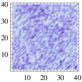
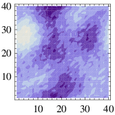
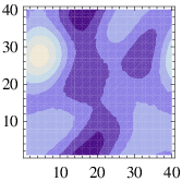
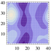
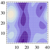
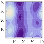
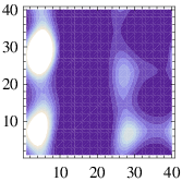
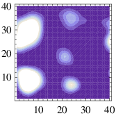
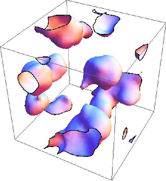
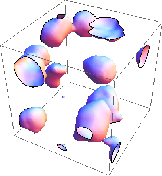
In Figs. 1 and 2 we show the fragmentation of the condensate. One can see the initial snapshot of a (nearly) homogeneous condensate in Fig. 1a. The process of fragmentation leads to islands with growing density contrast at later times, as shown in Fig. 1. Similar plots with different snapshots are shown in the 3D case, in Fig. 2, where one can see the fragmentation of the condensate into Q-balls. We can see how certain modes in the band of instability begin to grow leading to an eventual fragmentation of the condensate, and how these modes stop growing. At the same time, there is mode-mode mixing which excites higher- modes, and also affects the fragmentation process as shown in Figs. 1 and 2. The fragmentation does not happen isotropically, and coherent, macroscopic, non-spherical motions of the condensate create a quadrupole moment which leads to the creation of gravity waves.
In Fig. 3 we show the evolution of the energy density stored in the gravity waves with respect to the critical energy density of the universe at the time of production. We plot as a function of for GeV along with 2D slices and 3D isosurface plots for selected times, which correspond to the snapshots shown in Figs. 1 and 2. The dark grey dots in Fig. 3 are results of the 2D calculation, and the light grey dots are results of the 3D calculation, at the times that correspond to the snapshots in Figs. 1, and 2.
At the onset of fragmentation all the scalar modes are excited; however, as discussed above, only a narrow band of the initial perturbation spectrum becomes unstable. The band of instability obtained from numerical calculations is shown in Fig. 4. It agrees with our analytical estimate, see eq. (8). The gravitational waves spectrum is similar to that of the scalar perturbations, as shown in Figs. 4a, 4b. However the gravity wave spectra are flatter. We have multiplied the gravity wave power spectrum by to highlight the growing mode. We have found that the peak of the gravity wave spectrum is determined by the longest wavelength which is of the order of the time scale when the Q-balls form, i.e. , see Figs. 1 and 2. The growth eventually stops, once the fragmentation is near completion66 6 With our current simulation we are unable to determine the exact peak frequency for the gravity waves. We would require a larger box size, i.e. N=256, to demonstrate this initial frequency, which is beyond the scope of the current paper. For the moment we will restrict ourselves with an approximate analytical discussion on an observable frequency, see section VIII. .
In Fig. 5, we show the temporal evolution of the gravitational wave density for different values of the initial field perturbations, different values of and initial angular motion. In the perturbation plot, Fig. 5a, we find that the resulting gravitational wave energy density is independent of the size of the initial perturbation in the flat direction. The second plot, Fig. 5b, shows different values of determines how quickly the fragmentation proceeds, or the growth in the gravity wave density. We note that, when is set to zero, there is no growing mode, the condensate never fragments, and no gravity waves are produced.
VIII Observable signal
After they are produced, the gravitational waves are decoupled from plasma. Let us estimate the fraction of the critical energy density stored in the gravity waves today:
| (23) | |||||
where and are the present values of the scale factor and the Hubble expansion rate, and and are the respective values at the time of the fragmentation. The estimate obtained from our numerical results, is within one order of magnitude of the analytical estimates in eq. (19). LISA can detect the gravitational waves down to at mHz frequencies. One can estimate the peak frequency of the gravitational radiation observed today, which is determined by the initial frequency, . We obtain
| (24) | |||||
where we have assumed that (which also implies that one can neglect the expansion of the universe during the oscillations of the condensate). The numbers of relativistic degrees of freedom are , . Here the subscript “rh” denotes the epoch of reheating and thermalization, while the subscript “0” refers to the present time. The typical frequency of the gravity waves is be determined by the size of the fragmented regions. This is roughly given by the scale at which fragmentation happens, i.e. . This can be seen in our numerical results shown in Fig. 1 and Fig. 2. For TeV (the value of the reheat temperature is determined when the flat direction is responsible for reheating the universe [42, 8]), the frequency is of the order of Hz, which is in the right frequency range for LISA [27]. A higher temperature TeV corresponds to the frequency range, Hz. Signals in both of these ranges will be accessible to BBO [28] and Einstein Telescope [29]. Since the supersymmetry breaking scale is related to the energy in the condensate, as well as the reheating temperature, future gravity wave experiments could be in a position to probe supersymmetry breaking scale above 100 TeV, which beyond the reach of the Large Hadron Collider (LHC).
The spectrum of gravity waves produced by fragmentation is expected peak near the longest wavelength, of the order of the Q-ball size, which is . The relatively narrow spectral width will help distinguish this signal from the gravity waves generated by inflation [43], which are expected to have an approximately scale-invariant spectrum (and a smaller amplitude). It may be difficult, however, to distinguish this signal from that generated by a first-order phase transition [44], because both of these sources are expected to produce a relatively narrow spectrum determined by the Hubble parameter at the relevant time in the early universe. The gravity waves could also be generated in the electroweak-scale preheating. However, the amplitude of gravity waves expected in such a scenario [35] is considerably lower than that from the fragmentation of the supersymmetric condensate. LISA and BBO will be able to distinguish the gravity waves produced by fragmentation from those of point sources, such as merging black holes and neutron stars, which have specific “chirp” properties [45].
IX Conclusions
We have shown that the gravitational waves of observable amplitude could be produced when a homogeneous supersymmetric flat direction condensate fragmented into small lumps, i.e., Q-balls. The instability is a generic prediction for a supersymmetric flat direction in the early universe. The origin of the gravity waves is in the non-spherical anisotropic motions of the condensate that result from the growth of small initial perturbations.
Gravity waves with the energy fraction as large as can be generated with a peak frequency ranging from mHz to Hz, depending on the reheat temperature, which can vary in the range TeV. The signal in the mHz frequency range can be detected by LISA, while a higher frequency Hz is in the range of LIGO and BBO. The spectrum of gravity waves is different from many astrophysical sources identified by their chirp frequencies and from the gravity waves generated during inflation, which are stochastic waves with a scale invariant broad wavelength spectrum. However, a first-order phase transition in the early universe can produce a similar spectrum of gravitational radiation [44].
An observable amplitude of gravity waves can be produced by a class of flat directions which carry no net number and which are close to dominating the energy density of the universe at the time of fragmentation. Such flat directions are not responsible for generation of the baryon asymmetry via the Affleck-Dine scenario, although they may undergo a similar cosmological evolution as the flat directions discussed in connection with the matter-antimatter asymmetry. The asymmetry generated by these flat directions is destroyed by the electroweak sphalerons. Although the identification of the origin of the signal may not be unambiguous, detection of these gravity waves by LISA, BBO, or EINSTEIN could open a window on supersymmetry in the early universe even if it is realized at a very high energy scale.
X Acknowledgments
AK thanks M. Kawasaki and F. Takahashi for helpful discussions. The work of AK was supported in part by DOE grant DE-FG03-91ER40662 and by the NASA ATFP grant NNX08AL48G. AM would like to thank J. McDonald and D. Lyth and he is partly supported by “UNIVERSENET”(MRTN-CT-2006-035863) and by STFC Grant PP/D000394/1.
XI Appendix 1
Let us neglect any baryon number non-conservation and consider the homogeneous mode that obeys the classical equations of motion and and fluctuations about this classical solution, and . The equations of motion yield [5, 31]
| (25) | |||||
| (26) |
for the homogeneous mode, and
| (27) | |||||
| (28) |
for the fluctuations. Furthermore,
| (29) | |||||
| (30) |
Due to the conservation of the global U(1) charge in the physical volume, the solution has the property If the energy density of the scalar field dominates the universe, the homogeneous part of the field evolves as
| (31) | |||||
| (32) |
To find the most amplified mode, we use the ansatz:
| (33) | |||||
| (34) |
If is real and positive, these fluctuations grow exponentially, become nonlinear, and form balls [5]. Substituting these into eqs.(27) and (28), one obtains the following dispersion relation [31]:
| (35) |
where we have set . If one neglects the cosmological expansion and assumes for simplicity, one can reduce eq.(35) to an approximate simplified equation:
| (36) |
The perturbations grow exponentially if , which yields:
| (37) |
XII Appendix 2
For our numerical analysis it is convenient to define dimensionless variables:
| (38) |
which we will use to study gravity waves during the non-linear fragmentation of the condensate.
Writing , we obtain the equations for the homogeneous mode:
| (39) |
where , , and the prime denotes the derivative with respect to . For the fluctuations, one obtains
| (40) |
where denote the second derivatives with respect to and :
| (41) |
References
- [1] K. Enqvist and A. Mazumdar, Phys. Rept. 380, 99 (2003); M. Dine and A. Kusenko, Rev. Mod. Phys. 76, 1 (2004).
- [2] I. Affleck and M. Dine, Nucl. Phys. B 249, 361 (1985).
- [3] A. Kusenko, V. Kuzmin, M. E. Shaposhnikov and P. G. Tinyakov, Phys. Rev. Lett. 80, 3185 (1998); J. Arafune, T. Yoshida, S. Nakamura and K. Ogure, Phys. Rev. D 62, 105013 (2000); Y. Takenaga et al. [Super-Kamiokande Collaboration], Phys. Lett. B 647, 18 (2007); S. Cecchini et al. [SLIM Collaboration], Eur. Phys. J. C 57, 525 (2008); I. M. Shoemaker and A. Kusenko, Phys. Rev. D 78, 075014 (2008).
- [4] A. Kusenko, L. Loveridge and M. Shaposhnikov, Phys. Rev. D 72, 025015 (2005); A. Kusenko, L. C. Loveridge and M. Shaposhnikov, JCAP 0508, 011 (2005).
- [5] A. Kusenko and M. E. Shaposhnikov, Phys. Lett. B 418, 46 (1998).
- [6] K. Enqvist and J. McDonald, Phys. Lett. B 440, 59 (1998) [arXiv:hep-ph/9807269].
- [7] M. Laine and M. E. Shaposhnikov, Nucl. Phys. B 532, 376 (1998).
- [8] R. Allahverdi, K. Enqvist, J. Garcia-Bellido and A. Mazumdar, Phys. Rev. Lett. 97, 191304 (2006). R. Allahverdi, K. Enqvist, J. Garcia-Bellido, A. Jokinen and A. Mazumdar, JCAP 0706, 019 (2007) [arXiv:hep-ph/0610134].
- [9] R. Allahverdi, A. Kusenko and A. Mazumdar, JCAP 0707, 018 (2007).
- [10] K. Enqvist, S. Kasuya and A. Mazumdar, Phys. Rev. Lett. 90, 091302 (2003). K. Enqvist, A. Jokinen, S. Kasuya and A. Mazumdar, Phys. Rev. D 68, 103507 (2003). R. Allahverdi, K. Enqvist, A. Jokinen and A. Mazumdar, JCAP 0610, 007 (2006);
- [11] G. Rosen, J. Math. Phys. 9 (1968) 996; 9 (1968) 999; R. Friedberg, T. D. Lee and A. Sirlin, Phys. Rev. D 13, 2739 (1976); S. R. Coleman, Nucl. Phys. B 262, 263 (1985) [Erratum-ibid. B 269, 744 (1986)]; A. Kusenko, Phys. Lett. B 404, 285 (1997).
- [12] A. Kusenko, Phys. Lett. B 405, 108 (1997); Phys. Lett. B 406, 26 (1997).
- [13] G. R. Dvali, A. Kusenko and M. E. Shaposhnikov, Phys. Lett. B 417, 99 (1998).
- [14] K. Enqvist and J. McDonald, Phys. Lett. B 425, 309 (1998). K. Enqvist and J. McDonald, Nucl. Phys. B 538, 321 (1999).
- [15] K. Enqvist, A. Jokinen and J. McDonald, Phys. Lett. B 483, 191 (2000).
- [16] M. Axenides, S. Komineas, L. Perivolaropoulos and M. Floratos, Phys. Rev. D 61, 085006 (2000).
- [17] A. Pawl, Nucl. Phys. B 679, 231 (2004).
- [18] M. C. Johnson and M. Kamionkowski, arXiv:0805.1748 [astro-ph].
- [19] S. Kasuya and M. Kawasaki, Phys. Rev. D 61, 041301 (2000); S. Kasuya and M. Kawasaki, Phys. Rev. D 62, 023512 (2000); S. Kasuya and M. Kawasaki, Phys. Rev. Lett. 85, 2677 (2000).
- [20] T. Multamaki and I. Vilja, Nucl. Phys. B 574, 130 (2000). T. Multamaki and I. Vilja, Phys. Lett. B 535, 170 (2002). T. Multamaki, Phys. Lett. B 511, 92 (2001).
- [21] K. Enqvist, A. Jokinen, T. Multamaki and I. Vilja, Phys. Rev. D 63, 083501 (2001).
- [22] E. Palti, P. M. Saffin and E. J. Copeland, Phys. Rev. D 70, 083520 (2004). M. I. Tsumagari, E. J. Copeland and P. M. Saffin, arXiv:0805.3233 [hep-th].
- [23] L. Campanelli and M. Ruggieri, Phys. Rev. D 77, 043504 (2008).
- [24] T. Multamaki and I. Vilja, Phys. Lett. B 482, 161 (2000). T. Multamaki and I. Vilja, Phys. Lett. B 484, 283 (2000).
- [25] A. Kusenko and A. Mazumdar, Phys. Rev. Lett. 101, 211301 (2008) [arXiv:0807.4554 [astro-ph]].
- [26] http://www.ligo.caltech.edu/
- [27] http://lisa.nasa.gov/
- [28] G. M. Harry, et al., Class. Quant. Grav. 23, 4887 (2006) [Erratum-ibid. 23, 7361 (2006)]; V. Corbin and N. J. Cornish, Class. Quant. Grav. 23, 2435 (2006); http://universe.nasa.gov/new/program/bbo.html
- [29] http://www.et-gw.eu/
- [30] K. Enqvist, S. Kasuya and A. Mazumdar, Phys. Rev. Lett. 89, 091301 (2002).
- [31] K. Enqvist, S. Kasuya and A. Mazumdar, Phys. Rev. D 66, 043505 (2002).
- [32] M. Dine, L. Randall and S. D. Thomas, Nucl. Phys. B 458, 291 (1996).
- [33] M. Dine, L. Randall and S. D. Thomas, Phys. Rev. Lett. 75, 398 (1995);
- [34] T. Gherghetta, C. F. Kolda and S. P. Martin, Nucl. Phys. B 468, 37 (1996).
- [35] J. Garcia-Bellido, D. G. Figueroa and A. Sastre, arXiv:0707.0839 [hep-ph]. J. Garcia-Bellido and D. G. Figueroa, arXiv:0801.4109 [gr-qc].
- [36] J. F. Dufaux, A. Bergman, G. N. Felder, L. Kofman and J. P. Uzan, Phys. Rev. D 76, 123517 (2007).
- [37] R. Easther, J. T. Giblin, Jr., E. A. Lim, Phys.Rev.Lett.99:221301,2007. R. Easther, E. A. Lim, JCAP bf 0604, 010, (2006). R. Easther, John T. Giblin, E. A. Lim, Phys.Rev.D77, 103519, (2008). J. L. Cornou, E. Pajer and R. Sturani, Nucl. Phys. B 756, 16 (2006); A. Mazumdar and H. Stoica, arXiv:0807.2570 [hep-th].
- [38] S. Kasuya and F. Takahashi, JCAP 0711, 019 (2007) [arXiv:0709.2634 [hep-ph]].
- [39] A. G. Cohen, S. R. Coleman, H. Georgi and A. Manohar, Nucl. Phys. B 272, 301 (1986).
- [40] S. Kasuya and M. Kawasaki, Phys. Rev. D 64, 123515 (2001).
- [41] M. Kawasaki, K. Konya and F. Takahashi, Phys. Lett. B 619, 233 (2005) [arXiv:hep-ph/0504105].
- [42] R. Allahverdi and A. Mazumdar, JCAP 0610, 008 (2006).
- [43] A. A. Starobinsky, JETP Lett. 30, 682 (1979) [Pisma Zh. Eksp. Teor. Fiz. 30, 719 (1979)]. S. Dodelson, W. H. Kinney and E. W. Kolb, Phys. Rev. D 56, 3207 (1997); M. Maggiore, Phys. Rept. 331, 283 (2000); T. L. Smith, M. Kamionkowski and A. Cooray, Phys. Rev. D 73, 023504 (2006); arXiv:0802.1530 [astro-ph].
- [44] M. Kamionkowski, A. Kosowsky and M. S. Turner, Phys. Rev. D 49, 2837 (1994); C. Grojean and G. Servant, Phys. Rev. D 75 (2007) 043507 [arXiv:hep-ph/0607107]. C. Caprini, R. Durrer and G. Servant, Phys. Rev. D 77 (2008) 124015 [arXiv:0711.2593 [astro-ph]]. C. Caprini, R. Durrer, T. Konstandin and G. Servant, arXiv:0901.1661 [astro-ph].
- [45] B. J. Owen and B. S. Sathyaprakash, Phys. Rev. D 60, 022002 (1999).