Stability and dynamical properties of material flow systems on random networks
Abstract
The theory of complex networks and of disordered systems is used to study the stability and dynamical properties of a simple model of material flow networks defined on random graphs. In particular we address instabilities that are characteristic of flow networks in economic, ecological and biological systems. Based on results from random matrix theory, we work out the phase diagram of such systems defined on extensively connected random graphs, and study in detail how the choice of control policies and the network structure affects stability. We also present results for more complex topologies of the underlying graph, focussing on finitely connected Erdös-Réyni graphs, Small-World Networks and Barabási-Albert scale-free networks. Results indicate that variability of input-output matrix elements, and random structures of the underlying graph tend to make the system less stable, while fast price dynamics or strong responsiveness to stock accumulation promote stability.
pacs
64.60.aq(Networks), 64.60.De (Statistical mechanics of model systems), 89.65.Gh (Economics; econophysics, financial markets, business and management)1 Introduction
The goals of economic policy-makers include the promotion of economic growth and minimising the effects of down-turns. Consequently, understanding the causes of business cycles or fluctuations is vital to their efforts. Research into these causes has itself followed a cyclic pattern, often peaking soon after a major economic downturn [1].
A successful modern theory in this endeavour is the real business cycle (RBC) theory [2], according to which productivity shocks (i.e., changes in oil prices, technology and management strategy) induce fluctuations in capital accumulation, consumption and other economic indicators. Hence, the supply side of the economy is responsible for business cycles. Another major school of thought concerning business cycles is the New-Keynesian (NK) view [3], where consumer and investor pessimism are responsible for business fluctuations. A significant requirement on both RBC and NK views of economic cycles is that they must be ‘consistent with the micro-foundations of the macro-economy’ [4], i.e., that the study of global quantities needs to be linked to the behaviour of the microscopic constituents of the economy under consideration.
In this regard, statistical mechanics is an invaluable toolbox, as its approach rests on deriving laws for the macroscopic behaviour of many-body systems from their microscopic rules of engagement. Research along these lines has led to a theory for complex networks [5, 6, 7]. Herein, the attention has - to a certain degree - focused on the interplay between the topology of underlying interaction graphs and the robustness of systems of interacting agents. The broad scope of these studies includes ecological networks [8], metabolic networks [9] as well as studies of man-made networks such as the internet [10].
In [11] Helbing et. al. introduce a non-linear model for material flow between sectors of an economy. In their model, each material, or good is characterised by its inventory level, which, by virtue of a flux balance assumption, depends on the utilisation of good by other sectors in the economy and on the rate with which this good is consumed by external agents. Consumption rates, in turn, are influenced by the price of the goods via a non-linear demand function. The investigation of this model in [11] is based on a linear stability analysis of the stoichiometric sectorial utilisation matrix, using empirical data. The study concludes that the model does not require exogenous shocks to explain economic fluctuations. Moreover, the arrangement of economic units in a coupled network may lead to (undesired) global oscillations unless suitable countermeasures are taken, i.e. unless control policies are implemented which avert global instability and fluctuations. Other models of production networks include [12, 13, 14, 15, 16, 17, 18].
The aim of this present paper is to broaden the scope of the findings in [11] by considering ensembles of random input-output matrices instead of one single sample of empirical data. We focus on different ensembles of randomly assigned stoichiometric input-output matrices, and study the stability of a model whose dynamical properties are related to the ensemble of random matricies. As normally done, we map stability onto the eigenvalue spectra of the stoichiometric matrices. For networks with an extensive number of connections per node, the spectra can be found analytically using techniques from random matrix theory [19]. The stability of flow networks defined on finitely connected Erdös-Réyni (ER) graphs, small-word networks (SWN) and scale-free Barabási-Albert (BA) networks is addressed from numerical diagonalization of the corresponding stoichiometric matrices.
The remainder of the paper is organised as follows. In Sect. 2 we introduce the model. Sect. 3 then outlines the steps involved in characterising the system’s eigenvalues and hence its stability. This is followed by a detailed description of our results in Sect. 4. Finally, in Sect. 5 we provide concluding remarks and describe possible extensions for further work. Technical details concerning the calculation of the density and support of eigenvalues of Gaussian random matrices with extensive connectivity are presented in appendix A for completeness.
2 Model Definitions
2.1 Set-up of dynamical control policies
In this section we begin by describing the statistical model of material flow networks, which is based on the model introduced in [11]. One considers a system consisting of units of production. For each unit , we denotes by its rate of operation, given in units of delivery cycles per unit time. We also associate a unique commodity, denoted as good , with each unit. Each unit interacts with other units in the network by (i) producing/delivering goods and (ii) receiving/consuming goods from other units. The net flow, at time , of good through unit is , where is the difference between the amount of good received minus the amount of good produced by unit , per delivery cycle. The sign of the is here chosen as in [11]. The matrix is related to the aggregate Leontief input-output matrix [20]. The quantity may be positive (net production) or negative (net consumption). We will set in the following, reflecting the assumption that unit produces one unit of good per production cycle. If we assume that a fraction, of good is consumed by sinks outside the system, then the stock of good at time , i.e., is subject to the conservation law
| (1) |
We now focus on features that affect the rate of production of good at time . As per [11] the factors are two-fold: (i) if the current stock exceeds an optimal or equilibrium level, , the rate of production is reduced and vice versa. In operations management literature, such a strategy, which is referred to as ‘Constant Work-In Process’ [21], ensures that each economic sector (or factory) maintains and mitigates its inventory and backlog; (ii) if the rate of stock accumulation is growing, , this is an independent reason to reduce , and vice versa.
In addition to the aforementioned factors, each unit can potentially be subject to a control strategy that ensures if the rate of production exceeds an optimal value known a-priori, then will decrease, and vice versa. This strategy rests on the assumption that each production unit is subject to a budget constraint, limiting the range of production rates at which it can operate. Putting all these features together, we obtain, similarly to [11]
| (2) | |||||
where , and are sensitivity parameters. Note that is here assumed to be proportional to (i.e. relative changes in production rates are considered), ensuring that , if one starts with non-negative initial conditions.
For large economies there is an additional equilibrating mechanism, relating to the price of good at time , . As in [11] the factors that affect the price are taken to be identical to those affecting the production rates, and consequently we use
| (3) |
The pre-factor relates to the sensitivity of price change to the factors of influence. Specifically, is the price-responsiveness, i.e. low values of imply that prices of commodities relax quickly to their equilibrium prices, while large values of correspond to slow relaxation. In addition, it is also assumed that affects the consumption via a demand function, , which is non-linear. As per standard practice, is a monotonic decreasing function of . We will write
| (4) |
where are Gaussian random fluctuations and is the equilibrium value of external consumption of good . The demand function is modeled as
| (5) |
where and are non-negative real numbers. The equilibrium price is .
We will now specify choices for the network structure, i.e. the stoichiometric coefficients , and discuss their relation to the equilibrium values . In addition to these parameters, the model is defined by the variables . The and determine the response of external consumption to changes of price. The remaining variables lay out the control policies of the production units, and determine their dynamical adaptive behaviour. They are hence the key control parameters an economic policy-maker would adjust so as to maximise stability, and to minimise systemic fragility and undesired fluctuating or oscillatory behaviour.
2.2 Structure of interaction matrices
The freedom to choose appropriate units for allows us to re-scale the such that, the equilibrium fixed point (FP) solution of Eq. (1) is given by
| (6) |
i.e. we scale all such that for all . A similar approach was taken in [11]. We also assume that at equilibrium the external consumption of goods is homogeneous for all goods, i.e., . This simplification allows us to express Eq. (6) as
| (7) |
These conditions ensure that the overall flux of goods, including a non-negative outflow , is balanced, i.e. that no intrinsic creation of material occurs in the system (impossibility of the Land of Cockaigne [22, 23]).
We furthermore assume , i.e., the desired equilibrium stock level of good corresponds to the net outflow of good per unit time. Again, similar assumptions pertaining to have been made in [11].
While in [11] a specific input-output matrix, constructed from real-world data, was considered, we here focus on a synthetic stochastic setting, in which matrix elements are chosen to be random variables drawn from an ensemble. They are held fixed during the course of the temporal evolution of the . In the language of disordered systems theory the matrix elements are ‘quenched’ [24] variables. As mentioned earlier, represents the efficiency with which good is utilised to produce good . Changing is akin to structural changes in the production mechanism; adopting new technology, for example. It is reasonable to assume that such changes occur on a time-scale slower than that of our dynamical degrees of freedom, hence justifying our approach to regard the interaction matrices as quenched random variables. The paradigm of networked systems with randomly chosen interaction graphs and coupling constants will be discussed further below.
2.2.1 Structure of matrix elements
We are interested in the case where each unit interacts with a fraction of the other units. This consideration may be formalised by decomposing
| (8) |
where are quenched connectivity coefficients, determining the adjacency matrix of the flow network, and describes the amount of good utilised by unit .
The constraint in Eq. (7) is satisfied by constructing the as a linear combination of random variables . First, drawing the from some ensemble, and taking into account , we set for
| (9) |
The set in Eq. (9) denotes the elements on row such that . Analogous approaches have been taken in [25, 26]. This approach breaks down, however, if the elements on each row of matrix are identical. By providing a large enough variance for the distribution of we ensure that this case is avoided. Constrained random matrices have previously also been analysed in the context of glassy relaxation [27]. In this case, however, the formulation of the row constraint induced further correlations between off-diagonal and diagonal matrix elements. Our implementation, as discussed in Appendix A, avoids this issue, hence simplifying further analysis.
Below, we investigate the stability properties of the model for the cases of (i) dilute, but extensively connected and (ii) finitely connected ER random networks, (iii) networks exhibiting the small world property and (iv) scale-free networks.
2.2.2 Gaussian dilute ensemble
We assume , i.e., we consider the underlying network (as defined by the adjacency matrix) to be undirected. Directionality in the resulting material flow is modelled by allowing the utilisation parameters to be asymmetric, i.e by allowing for cases in which , as we will detail below. The connectivity coefficients are drawn from the following distribution:
| (10) |
where is the average connectivity per production unit.
In what follows we consider the limit of so-called ‘extreme dilution’ [28], where and , while the ratio tends to zero, i.e. . This may be achieved by allowing, for example . This assumption has important implications for the structure of the adjacency graph. Firstly, each node in the graph will be connected to a vanishing fraction of the total number of nodes. Secondly, the length of a typical loop is [29]. Thus, taking , the probability of finding loops of finite length tends to . The environment about each node is thus locally tree-like.
The utilisation parameters are also taken to be quenched. To allow for a well-defined thermodynamic limit, and , the mean and variance of need to scale suitably with . Specifically,
| (11) |
leads to a mathematically non-trivial regime, where we choose the to be Gaussian random variables of zero mean and a variance of order [30]. Specifically, the are independent in pairs and for and and have the following moments:
| (12) |
The parameter describes the degree of correlations, with fully symmetric interactions given by . The eigenvalue spectra of such Gaussian random matrices can be computed fully analytically, see for example [31] for results regarding fully connected Gaussian ensembles. The extension to the dilute, but extensively connected case respecting the constraint of Eq. (7) is straightforward, we report some steps of the corresponding calculation in Appendix A. Our investigation of the stability properties of such flow networks can hence be carried out analytically to a large degree.
2.2.3 Gaussian finitely-connected ensemble
We consider to be distributed according to Eq. (10), and continue to take . However, the average connectivity, scales as , while we still consider the thermodynamic limit . The statistics of the are again those indicated in Eqs. (11) and (12).
This scaling of and to be complicates the analytical characterisation of the statistics of eigenvalues. Recent efforts [32, 33, 34, 35, 36, 37, 38, 39] have lead to an implicit characterisation of eigenvalue densities in terms of population dynamical equations, often used in the context of the cavity method. In our analysis of finitely connected cases, we do not resort to such tools, but evaluate the corresponding eigenvalue statistics via explicit numerical diagonalization.
2.2.4 Small world graphs
Another ensemble we consider is that where the define a Small-World Network (SWN) [40, 41]. Under this paradigm, one starts from a network in which units are arranged on a one-dimensional lattice with periodic boundary conditions (i.e. a ring). Each unit is then connected to () of its nearest-neighbours (i.e. neighbours to the right and neighbours to the left of the unit on the ring). In the context of an economy, ‘near’, in a stylistic sense, models geographic or economic proximity, e.g. two production units within a country. The total number of undirected links in the system is .
Based on the algorithm proposed in [40], starting with the first node and its pre-exiting nearest-neighbours links in a clock-wise direction, we re-wire each link with probability , i.e., the nearest-neighbour link is removed and replaced by a link to another randomly selected node. In an economic context these re-wired links may, for example, represent economic interactions of a given unit with units at long ‘distances’, e.g. in a different country. This procedure is iterated for each node. At the end, the total number of links is still the same, while the number of re-wired, or long-ranged links is .
An alternative algorithm is that proposed in [41], where starting with the first node, for each of its pre-existing neighbour-interactions, we add an additional link to another node with probability . One then proceeds with the second node and so on. At the end of the procedure, the expected coordination number per node is .
Couplings strengths are given by , where and the moments of is given by Eq. (12).
Once again, since and scale as , an analytical characterisation of the statistics of eigenvalues of large SWN is difficult. We here limit ourselves to numerical diagonalization when addressing small world networks. We also compare results obtained for the two construction algorithms.
2.2.5 Scale-free networks
As a final example we study the model on a scale-free network. To this end we employ a growth process as proposed in [42] and construct the underlying adjacency matrix as follows: the seed of the growth process is a network composed of two nodes, , with . At each time-step one further node is added to the network, and connects to one of the already existing nodes () by preferential attachment, i.e. the probability of attaching to node is proportional to the degree of node . As shown in [42] this leads to a scale-free degree distribution asymptotically, i.e. in the limit of infinite network size. In our simulations this scaling is reproduced faithfully, yielding e.g. exponents of at system sizes of . In our analysis below we will use smaller networks of typically nodes for computational reasons (the stability analysis entails diagonalization of matrices of size which can be costly if a large number of samples needs to be considered). For such sizes a scale-free degree distribution with a slightly smaller scaling exponent is found. We once more take , where and the moments of are given by Eq. (12).
2.3 Paradigm of random network models
The model as we use it here assumes that the interactions between units in the system constitute a random graph in which the presence or absence and the weight on each link existing link are quenched random variables, i.e., drawn from some distribution and then kept fixed in time. Such random structures can, at best, be seen as a minimalist approximation to real-world flow networks which are generally not random in their structure, and which can emerge from a growth or evolutionary process in which e.g. certain production units go ‘extinct’ (bankrupt) and where new units join over time.
Nevertheless, studying quenched random structures allows for a meaningful abstraction of real-world phenomena and analytical tractability of the mathematical model. Such approaches have been used in a variety of different contexts such as neural networks [43, 44], economic activity [25, 45] and ecology [46, 47], amongst others. In ecology in particular an ongoing debate on the effects of complexity on the stability or otherwise has been sparked by the study of random community models, and such model systems are under active investigation e.g. in [48, 49]. The random ensembles of graph structures and distributions of couplings we use in our work are characterised by parameters such as the mean connectivity or variance of the randomly drawn elements in the Leontief matrix. The analysis thus allows for a specific characterisation of the effects of such parameters on the stability or otherwise of the system, and on its dynamical behaviour. In subsequent work one can then build on this approach and add more realism by allowing the graph itself evolve in time [50, 51].
A further drawback of the present model is the assumption that equilibrium values are controlled externally (e.g. set to unity), and are not outcomes of the dynamics itself. Nevertheless, it was shown in [45] that the correlation of fixed-points values of the microscopic variables with coupling matrix elements in models with random interactions may often be ignored for the consideration of stability properties of random coupling models. Our lines of reasoning follow this approach.
3 Model Solutions
Here we investigate the properties and solutions to the model presented in Sect. 2. As in [11] we henceforth assume homogeneous model parameters, , , and and use the demand function,
| (13) |
At the FP we take and assume that .
3.1 Linear Stability Analysis
We now investigate how the stability of the fixed-points depends on model parameters. To this end we perform a linear stability analysis, i.e. the eigenvalues of the Jacobian of the systems are used to characterise the dynamical behaviour of the system when subjected to external perturbations.
The linearization of the dynamical system about the fixed-points is given by
| (14) | |||||
| (15) | |||||
| (16) |
We note that the control policy has dropped out of our equations. While the system has dimension 3, its rank is only 2. Consequently, of its eigenvalues vanish. We denote the remaining 2 eigenvalues by with . Labelling the eigenvalues of the stoichiometric matrix by , for , we obtain, similar to [11]
| (17) |
where,
| (18) | |||||
| (19) |
Due to the eigenvalues at zero, the FPs of our system can either be marginally stable or unstable. Such zero modes are not unusual in storage systems of the type we are considering here, and reflect the effects of an ‘integrating’ behaviour of the buffers, which might cause the operating point to drift in time [52]. Following [11] we hence characterise the stability or otherwise of the system in terms of the remaining eigenvalues. Eqs. (17) - (19) relate the eigenvalues of the full system to those of the interaction matrix, . In what follows we show that the stability of the full system depends on the statistics of the only through the support of its spectral density.
3.2 Density of eigenvalue for the Gaussian dilute ensemble
We here establish the average density of eigenvalues, , , for an ensemble of dilute real Gaussian random matrices, , defined via Eq. (9), where the ’s and ’s are drawn according to Eq. (10) and Eqs. (11)-(12), respectively. The density of eigenvalues is given by
| (20) |
where the denotes an ensemble average. Following the lines of Sommers et al [31], and referring to the real and imaginary parts of by and , respectively (i.e. ), we obtain
in the thermodynamic limit, . We have here written and . The eigenvalues are hence uniformly distributed in the ellipse with major and minor axis given by and , respectively. These results accurately match numerical results, and while we will not enter the details of the derivation of Eq. (3.2) in the main text, Appendix A contains some intermediate steps of the computation. In particular, with the scaling of couplings as chosen above, the result is independent of the connectivity parameter .
3.3 Mapping the eigenvalue support
The stability or otherwise, and dynamical behaviour of the flow system is characterised by the eigenvalue, Eq. (17), of the system with the largest real part. We denoted this eigenvalue by . Working in the thermodynamic limit and considering the map , defined by Eq. (17), is found to lie on the image of the boundary of the ellipse defined by Eq. (3.2). Thus in order to determine the long-term dynamical behaviour of the system only the image of this boundary needs to be considered.
Fig. 1 verifies the validity of this mapping and compares the analytically obtained boundary of the spectrum of the system against results from direct numerical diagonalization. The crosses in the figure are from numerical diagonalization of the system, while the solid line is from mapping of the boundary via
| (25) | |||||
| (26) |
where and .
Fig. 1 demonstrates that the analytical theory captures the boundary of the spectrum faithfully, and allows one to make statements regarding . The identification of this eigenvalue may be unique only up to complex-conjugation.
We note that the density of within the predicted support is not uniform. This is due to a non-trivial Jacobian of the transformation
| (27) |
However, randomly sampling according to Eq. (3.2) and applying Eq. (25)-(26), yields, in the large limit, a dense scattering of within the mapped boundary.
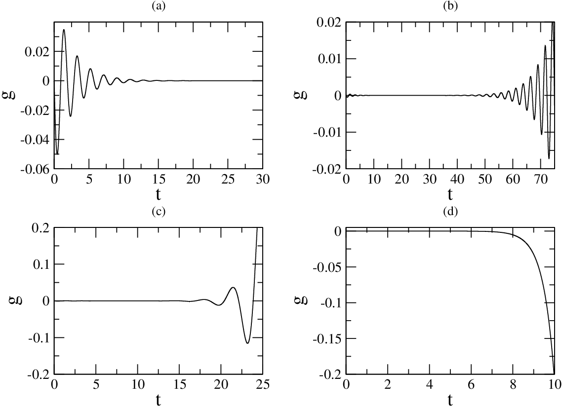
The sequence of spectra shown in Fig. 1 reveals two different transitions of the dynamical behaviour of the system as the model parameter , i.e. the variability of elements in the coupling matrix, is increased. At small (see panel (a)) one finds and , indicating damped oscillations. As is increased (see e.g. panel (b)) the real part of becomes positive with the imaginary part still remaining non-zero. This corresponds to growing oscillations. As is increased further continues to display a positive real part, but it’s imaginary part vanishes, i.e., panel (d). Hence the system is in an exponentially growing phase, where no oscillations are to be expected. In order to verify that these eigenvalue distributions capture the stability properties and dynamical behaviour of the system correctly, we have integrated the linearised dynamics, Eqs. (14, 15,16) numerically, initialising the system close to its fixed point. Fig. 2 shows the resulting behaviour of as a function of time, and results confirm the transitions predicted in by the eigenvalue distributions shown in Fig. 1.
We discuss the phase behaviour in more detail in the next section, and focus on studying how the different model parameters affect the stability or otherwise of the model.

4 Results
In the space of control policies, i.e., , , , , , and parameters and characterising the statistics of the input-output matrix as well as in dependence on the structure of the underlying network, we ask, what policies promote stability? Due to the large number of model parameters, our investigations necessarily focus on a few specific cuts in parameter space. While this is cannot be an exhaustive enumeration of effects of all different model parameters, we find that the behaviour exhibited in these phases is rich and informative regarding the impact of policy changes.
For a given set of parameters, the system’s FP is meta-stable if or is otherwise unstable. The trajectories to the FP are damped if . If has a non-zero imaginary part, then the trajectories are characterised by oscillations.
We adopt the following notation to distinguish the different phases: (i) OD: oscillatory decay ( and ), (ii) OG: oscillatory growth ( and ), (iii) ED: exponential decay ( and ) and (iv) EG: exponential growth ( and ).
Finally, for simplicity, we take . In all tested cases for one finds that . Consequently, in that case, the regions in the phase plane will be either ED or EG.
4.1 Gaussian dilute ensemble
4.1.1 Preliminary observations: effects of couplings strength and symmetry of interactions
Fig. 3 plots the resulting phase boundaries in the (,) plane. Crossing the lower curve from below switches from negative (FP is meta-stable) to positive (FP is unstable). The upper curve separates regions with zero and non-zero , respectively, with oscillatory behaviour found below and damped trajectories above the line. Hence, the phase space is divided into three regions, OD, OG and EG, and the transitions reported in Figs. 1 and 2 correspond to moving along a vertical line upwards in the phase diagram, at fixed .
For a given degree of symmetry between matrix elements, i.e., fixed , increasing the variability between interactions, i.e., , pushes the system from a stable phase with damped oscillations to an unstable phase. If the matrix elements are fully symmetric, then the unstable phase is always characterised by exponential growth. However, for intermediate degrees of symmetry, there exists a range of for which one observes growing oscillations. The behaviour depicted extends into the negative region. In particular, as approaches the upper curve becomes increasingly steep and diverges for , where the unstable phase is always characterised by growing oscillations.

Our preliminary observations are: (i) increasing the variance of couplings makes the system more unstable and (ii) as couplings becomes more symmetric the intermediate OG phase diminishes and is absent in the fully symmetric case. In what follows we show that these findings are robust under the variation of model parameters.
4.1.2 Effects of price relaxation rate
Fig. 4 plots phase boundaries in the (, ) plane, for different values of the price-responsiveness policy . We find that the qualitative structure of the phase diagram in Fig. 3 remains unchanged as is varied, i.e., for different price relaxation regimes.

For a given , the critical value , separating the OD and OG phases, decreases as is lowered. Moreover, the curve, as a function of , switches from a monotonic increasing to a decreasing function. We conclude that quickly evolving prices, i.e., large promotes stability.
Fig. 5 illustrates this further by plotting phase boundaries in the (, ) plane for different values of . The phase space is once again divided into the three distinct regions. The curve is an increasing function of . As we increase the OG regions diminish, until for the two phase boundaries coincide exactly with each other, excluding the OG region from the parameter space. We observe a direct transition from OD to EG. As previously mentioned, increasing moves the system from a stable to an unstable phase.

The results discussed so far are derived from the analytically known spectra of Gaussian random matrices and large connectivity in the limit of infinite system size. Only in this limit are analytical results available. In order to assess the behaviour of finite systems we consider the probability that a finite system finds itself in either of the four phases as a function of the model parameters. These probabilities were computed from a numerical diagonalization and a subsequent identification of the largest eigenvalue.
Fig. 6 reports the relative frequency with which each phases occurs (phases not reported in the figure are not observed in the simulation). The behaviour of the finite system follows that predicted by the theory to a good accuracy. Discrepancies occur in a parameter regime where the theory predicts exponential growth. Here, the analytically predicted largest eigenvalue is real and positive. In finite systems however, largest eigenvalues with a non-zero imaginary part may be found due to finite-size fluctuations. We observe a similar discrepancy in the lower-right panel of Fig. 1, where the theory predicts a real-valued largest eigenvalue, but explicit diagonalization at finite sizes delivers eigenvalues with non-vanishing imaginary values. We attribute the smearing-out of the OG to EG transition and co-existence of both phases at large in the upper panel of Fig. 6 to this finite-size effect.

4.1.3 Sensitivity of production rate to stock accumulation
The parameter is a measure for the sensitivity of a unit’s rate of production to its rate of stock accumulation . In order to characterise the effects of this control policy, we compute in Fig. 7 the phase diagram in the () plane for different values of . For any degree of asymmetry in the couplings, we find that increasing the sensitivity of the production rate to stock accumulation enhances stability - in panels (a)-(c) the area covered by the OD phase increases as we increase . For we begin to observe the ED phase as well. As the sensitivity is increased further the lines separating ED-OD and OG-EG transitions converge until the system experiences a direct transition from the ED to EG phase.

Finally, we further support our findings on the roles played by and in promoting stability, by investigating the special case of fully symmetric matrix elements, . Here all are real and in this case one can show that is real and negative whenever the following two conditions are satisfied simultaneously:
| (28) |
and
| (29) |
Here is the real part of the eigenvalue of the Leontief matrix, giving rise to the relevant eigenvalue determining the stability of the system. A condition similar to the latter is also found in [11]. For further illustration, Fig. 8 shows the resulting phase diagram in the (, /) plane. The vertical line is where is equal to the right hand side of Eq. (28), separating the unstable EG phase at large from the stable ones at smaller values of . If prices evolve sufficiently fast (), increasing stabilises the system further (at fixed ) by supressing oscillations, as seen in Fig. 8. In [11] a related phase diagram is shown, based on stochastic modifications of an input-output matrix drawn from real world data.
Evaluating Eq. (29), which defines the phase lines separating the OD from the ED phase, requires the knowledge of as a function of the model parameters. This relation may in general be somewhat intricate, at however one has . The two dashed lines in the figure correspond to Eq. (29) evaluated for values of at the limits of this interval, hence limiting the location of the phase transition separating the ED from the OD phase. The actual transition point is found to lie between these boundaries (solid line).

4.2 Gaussian finitely-connected ensemble
While the results presented for the Gaussian ensemble with a large connectivity are rich, the assumption that production networks display such topology is admittedly a very stylized one, chosen because of the available analytical results of the spectra of the corresponding couplings matrices. More realistic choices might correspond to networks in which each node is connected, on average, to a finite number of other nodes, . In order to study such models we next switch our attention to finitely connected ER graphs as introduced in Sec 2.2.3.
Results for the density of eigenvalues for such couplings matrices are so far only available for fully symmetric couplings and have been expressed using approximation schemes, such as the single defect approximation (SDA) [53] and effective medium approximation (EMA) [35]. Other approaches, motivated by the statistical mechanics analysis of spin-glass type systems express the density via cavity equations [37] and as the solution to population-dynamics equations [36, 38].
For asymmetric random matrices, however, similar results are not yet available. It has nevertheless been argued [54] that for any finitely connected ER random graph the tails of the spectra is characterised by Lifshitz tails; hence the entire complex plane serves as the support. While most eigenvalues are found concentrated around an origin, there are outlier eigenvalues. For finite sized systems these outliers may have a significant impact on the dynamical behaviour of the system

Fig. 9 plots for finite systems at an average connectivity of the probability that the system finds itself in a particular configuration, as a function of . For small , the system is unstable and in the EG phase. However, as we increase and allow for faster price relaxation dynamics, the system first enters the unstable OG phase and later makes a transition to the stable OD phase. When tested against and we found that the location of the transition points vary by only . In particular, this point is in good agreement with that for the fully connected system as given in Fig. 5 and depicted in Fig. 9 by the vertical dashed lines. This is a result of our scaling of the matrix interaction term as .
If we remove this particular scaling of the couplings the behaviour of the system becomes dependent on the mean connectivity of the underlying network, see Fig. 10. As increases, the system tends to become more unstable. In the case of full asymmetry a transition between an oscillatory decaying phase and an oscillatory unstable phase is found. If interactions are fully symmetric, then a we increase we system switches from the OD phase to a state dominated by the EG phase with high probability.

4.3 Small world networks
In considering the SWNs ensemble, one introduces two new parameters to the system: (i) number of nearest-neighbours links, in the initial network, and (ii) the amount of long-range links, parametrised by model parameters and , as explained in Sec. 2.2.4.
Under the first variant for the algorithm, [40], each nearest-neighbour link is re-wired with probability . In Fig. 11 we show that as tends to 1, i.e., the network moves from a structured state to a random one, the system becomes more unstable. Initially the system finds itself in the OD phase, but as increases we observe co-existence with the OG phase.

For the second variant to construct the network, [41], Fig. 12 plots the probability a stable state, i.e., is achieved as a function of the rate with which additional links are introduced into the nearest-neighbour network. As increases, the system becomes more unstable. Similarly, stability is reduced as the number of nearest-neighbours, , is increased. Thus, in accordance with results in Sec 4.2, it is mostly the total number of links in the system that (all other parameters remaining the same) controls the stability of the network.

4.4 Scale-free networks
Results for scale-free networks are shown in Fig. 13 for a specific choice of parameters. We show the probability as a function of the coupling strengths for both BA like networks and ER graphs. In both cases the model is set up such that the average degree of nodes is . As in previous cases, the system size is , and results in a scaling exponent of approximately in the BA-case. The remaining parameters are as indicated in the figure caption.
The upper panel reveals that for both types of the underlying adjacency matrix, the system exhibits a stable phase at low variability of elements of the Leontief-matrix, i.e. at low values of virtually all randomly drawn instances are found to be stable. Note that randomness here refers to both, the underlying graph and the coupling strengths along the links. Both systems exhibit a crossover to an unstable phase as matrix elements become more diverse. Crucially however the probability of finding a stable instance of the flow network is consistently higher in the case of BA-like graphs as compared to ER-networks. Near approximately this effect can be significant, raising the probability of being stable from about per cent (ER) to per cent (BA). This observation is further illustrated in the lower panel of Fig. 13, where we depict the real part of the relevant eigenvalue . In the stable regime the relaxation time, or resilience of the network against perturbations is given by , and since is consistently higher (in the stable phase) in the BA case as compared to the ER case we conclude that the BA network appears to be more resilient against external fluctuations than the ER graph. Similar statements can be made in the unstable phase, where for both types of networks, but where this real-part is consistently larger in the ER case compared to the BA network. Hence perturbations to flow-networks defined on ER graphs show a much larger growth rate as compared to BA graphs. We would here like to stress that the observations presented in Fig. 13 are only for one specific combination of model parameters, and that the above statements are hence valid only pending a systematic investigation of other circumstances. Still, the chose example illustrates that the structure of the underlying adjacency matrix can be relevant and that scale-free degree distributions may potentially promote stability in the context of the present model.

5 Conclusion
We have studied the stability and dynamical properties of a material flow system defined on a variety of random and complex network structures. Results from random matrix theory have been used to address models in the extremely dilute limit with Gaussian couplings, provided coupling strengths are scaled appropriately with the mean connectivity 11 1 However, it should be noted that the assumption needed to carry through the RMT as described in this paper is rather than sparseness. Hence, the analysis applies to networks with non-sparse connectivity with as well.. Our theoretical findings are here in very good agreement with results obtained from direct numerical diagonalization, and indicate complex phase diagrams in dependence on the network structure, symmetry or otherwise of input and output matrices and most crucially on parameters characterising the external control policies applied to the network.
The analysis of Gaussian dilute networks reveals the following key findings: (i) Increasing the variance between matrix couple elements makes the system unstable, (ii) quickly evolving prices are conducive to a stable environment, (iii) greater sensitivity of the rate of production to stock accumulation can also yield greater stability by suppressing oscillations. The role of the coupling symmetry is more intricate: if prices adjust slowly or the rate of production is weakly sensitive to stock accumulation, then increasing the symmetry between the underlying network couplings makes the system more stable. For quickly evolving prices or high sensitivity, however, increasing the symmetry results in a more unstable system.
An investigation of finitely connected networks allows us to study the question of how the mean degree of nodes in the flow network affects its stability. At fixed connectivity we find that symmetry in interactions and a high degree of variability in interaction strengths reduces the extent of the stable region in parameter space, as in the fully connected model. Increased connectivity adds to the variance of coupling strengths, and hence again promotes instability.
Studying flow dynamics on SWNs reveals that an increased the re-wiring probability makes the system more unstable if prices evolve slowly. Thus, networks with a regular structure, as opposed to random networks, promote stability. Similarly, increasing the number of nearest-neighbour links has a marked impact of making the system more unstable for slow price dynamics. Finally, we have interaction graphs of BA type, and our results indicate that the underlying scale-free structures may promote stability.
The route taken in this paper was to study flow systems defined on random networks. Randomness here refers to both stochasticity in the strengths of interactions (entries in the Leontief matrix), but also to the presence or absence of links between individual units of production. The latter type of stochasticity is a common tool in the theory of complex networks, while the former has been applied in a variety of contexts, e.g. in ecology [46, 47], linear economies [55], evolutionary game theory [56, 57]. Real-world production networks are of course not random, neither in their structure nor in the magnitude of inter-unit dependencies. Still, choosing ensembles of random networks allows one to unearth general principles that determine the stability or otherwise of such models, e.g. our study consistently seems to indicate that an increased variability of elements in the Leontief input-output matrix generally induces instability. This leads to the obvious task of identifying analogous measures of variability in real-world production networks, and to verify whether or not such a correlation between complexity and stability can be confirmed.
It is also legitimate to ask what values the various model parameters would take in real-world production networks? To sensibly answer this question one must analyse real-world data, which is beyond the scope of the present paper. Statistics for and can be obtained by analysing real-world data such as used in [11]. Positive values of indicate a tendency towards two-cycles in the production network (e.g. A uses B and B uses A). Such direct cycles are presumably unlikely and we expect small values, more realistic. Control policies such as the price responsiveness are dynamic quantities. This makes their direct measurement difficult, as the temporal behaviour of real systems would have to be probed. While calibrating the model is a necessary future step, the focus of the present paper is on the statistical mechanics analysis and phase behaviour of the model. The contribution of the present paper is a comprehensive analysis, outlining the complex interplay between relevant parameters, against which real-world scenarios may be placed.
Further directions of future research and modelling attempts include the intricate dynamics of evolving production networks, in which the underlying graph is a function of time itself, leading to a system in which discrete degrees of freedom (absence or presence of links) interacts with continuous ones (e.g. production rates defined on the nodes of the network). Such systems are known as hybrid complex systems [58]. Depending on the separation of time scales, different types of dynamical behaviour might then to be expected, with the freedom of removing or adding links potentially helping to stabilise the model.
Acknowledgements
This work was initiated at the Abdus Salam International Centre for Theoretical Physics, Trieste, Italy, which the authors would like to thank for hospitality. Fruitful discussions with Stefan Lämmer, Reimer Kühn and Andrea De Martino are gratefully acknowledged. TG is an RCUK Fellow (RCUK reference EP/E500048/1).
Appendix A Random Matrix Theory
Following lines of reasoning provided in [31] and employing an electrostatic analogy, the starting point to evaluate the spectra of eigenvalues is the Green’s function,
| (30) |
where denotes the eigenvalues of matrix . The real and imaginary parts of Eq. (30) relate to an electric field, with charges at points . We can define a potential,
| (31) |
where is the complex-conjugate of eigenvalue . Eq. (31) satisfies, for , . The average density of eigenvalues was shown to be related to averaged over an ensemble of matrices , i.e., the disorder average, , via Poisson’s equation,
| (32) |
where, . The righthand-side of Eq. (32) vanishes if satisfies the Cauchy-Riemann conditions and is an analytical function in the complex plane. In other words, we can re-interpret as the measure of non-analyticity in .
As a first step, one must regularise the logarithm in Eq. (32) by introducing a positive infinitesimal . This ensures that the matrix whose determinant we seek is positive definite; consequently one may represent the determinant [59] as an integral over complex variables,
| (33) | |||||
where and .
The next step is to perform the average via the replica trick [60], , the result of which may be solved in the limit via the saddle point technique. However, as noted in [61], the integrand that one evaluates has its extremum for order-parameters that do not depend on the replica index. As a result, may be calculated formally by setting .
The average is facilitated by linearising terms quadratic in via a complex Hubbard-Stratonovich transformation,
| (34) | |||||
where the disorder terms are restricted in
| (35) |
and
| (36) |
for off-diagonal elements, while . The elements are a linear combination of Gaussian random variables and we verify that up to leading ,
| (37) |
We perform the average of the and in the usual manner; for details refer to [30].
We note that in Eq. (34) if we rotate all and , i.e., multiply them with that has unit modulus, the integral remains unchanged. More precisely, the terms in the exponential in Eq. (34) are invariant under this transformation. In our case, we must take terms of the form , , , , and all to be equal to zero. We consequently introduce order-parameters
| (38) | |||||
| (39) |
Consequently, Eq. (34) reduces to
| (40) | |||||
We introduce the order-parameter definitions Eqs. (38) - (39) into Eq. (40) via Dirac functions. This allows us to perform the integrals over and using Gaussian identities, which yields
| (41) |
where,
| (42) | |||||
| (43) | |||||
| (44) |
and denotes the integral over variables the order parameters and their “hatted” conjugate variables, which are a consequence of a Fourier representation of the Dirac functions.
The average potential, is related to the saddle-point value of the function . We proceed by eliminating the conjugate variable by requiring stationarity. Next, we introduce and eliminate using the stationarity condition .
| (45) | |||||
In the limit , we may distinguish between two possibilities; may take a maximum at or there may be an extremum for some . Considering first , Eq. (45) resolves to an analytical function in the domain of ; hence, and .
In the case one obtains an extremum for , with , we obtain saddle point equations
| (46) | |||||
| (47) | |||||
| (48) |
Evaluating at this saddle point and employing Eq. (32) we obtain the average density, , which is valid in the region , i.e.,
| (49) |
where and .
References
- [1] A Abel and B Bernanke. Macroeconomics. Addison Wesley, 2003.
- [2] C Plosser. Understanding real business cycles. The Journal of Economic Perspectives, 3:51–77, 1989.
- [3] R Farmer and J T Guo. Real business cycles and the animal spirits hypothesis. Journal of Economic Theory, 63:43–72, 1994.
- [4] G Mankiw. The reincarnation of keynesian economics. European Economic Review, 36:559–565, 1992.
- [5] R Albert and A L Barabási. Statistical mechanics of complex networks. Reviews of Modern Physics, 74:47–97, 2002.
- [6] S N Dorogovtsev and J F F Mendes. Evolution of Networks: From Biological Nets to the Internet and WWW. Oxford University Press,US, 2003.
- [7] M E J Newman, A L Barabási, and D J Watts. The Structure and Dynamics of Networks. Princeton University Press, US, 2006.
- [8] B Drossel and A J McKane. Handbook of Graphs and Networks, chapter Modelling Food Webs. Wiley-VCH, 2003.
- [9] U Alon. An Introduction to Systems Biology: Design Principles of Biological Circuits. Chapman and Hall, 2006.
- [10] S Bornholdt and H G Schuster. Handbook of Graphs and Networks: From the genome to the internet. Wiley, 2006.
- [11] D Helbing, S Lämmer, U Witt, and T Brenner. Network-induced oscillatory behavior in material flow networks and irregular business cycles. Physical Review E, 70:56118, 2004.
- [12] A Ponzi, A Yasutomi, and K Kaneko. A non-linear model of economic production networks. Physica A, 324:372–379, 2003.
- [13] D Helbing, S Lämmer, T Seidel, P Seba, and T Platkowski. Physics, stability and dynamics of supply networks. Physical Review E, 70:066116, 2004.
- [14] A Ponzi, A Yasutomi, and K Kaneko. Complex dynamical behaviour in economic production networks. Journal of Economic Behavior and Organization, 61:729–749, 2006.
- [15] G Weisbuch. Self-organized patterns in production networks. Complexus, pages 217–227, 2005.
- [16] G Weisbuch and S Battiston. Production networks and failure avalanches. arXiv:physics/0507101v1, 2005.
- [17] M D Köenig, S Battiston, and F Schweitzer. Modeling evolving innovation networks. arXiv.org:0712.2779, 2007.
- [18] M D König, S Battiston, M Napoletano, and F Schweitzer. On algebraic graph theory and the dynamics of innovation networks. Networks and Heterogeneous Media, 3:201–219, 2008.
- [19] M L Mehta. Random Matrices (3rd ed.). Elsevier/Academic Press, Amsterdam, 2004.
- [20] W Leontief. Input-Output Economics. Oxford University Press, 1986.
- [21] M Spearman, D Woodruff, and W Hopp. Conwip: a pull alternative to kanban. International Journal of Production Research, 28:879–894, 1990.
- [22] M Morishima. On the two theorems of growth economics: A mathematical exercise. Econometrica, 33:829–840, 1965.
- [23] K Lancaster. Mathematical Economics. Dover Publications, New York, 1987.
- [24] M Mézard, G Parisi, and M A Virasoro. Spin Glass Theory and Beyond. World Scientific, Singapore, 1987.
- [25] A De Martino, M Marsili, and I Pérez Castillo. Statistical mechanics analysis of the equilibria of linear economies. Journal of Statistical Mechanics: Theory and Experiment, 2004:P04002, 2004.
- [26] Andrea De Martino, Private communication (2007).
- [27] A J Bray and G J Rodgers. Diffusion in a sparsely connected space: A model for glassy relaxation. Physical Review B, 16:11461–11470, 1988.
- [28] J P L Hatchett and R Kühn. Effects of economic interactions on credit risk. Journal of Physics A, 39:2231–2251, 2006.
- [29] B Derrida, E Gardner, and A Zippelius. An exactly soluble asymmetric neural network model. Europhysics Letters, 4:167–173, 1987.
- [30] K Anand and R Kühn. Phase transitions in operational risk. Physical Review E, 75:016111, 2007.
- [31] H J Sommers, A Crisanti, H Sompolinsky, and Y Stein. Spectrum of large random asymmetric matrices. Physical Review Letters, 60:1895–1898, 1988.
- [32] G J Rodgers and A J Bray. Density of states of a sparse random matrix. Physical Review B, 37:3557–3562, 1988.
- [33] G Biroli and R Monasson. A single defect approximation for localized states on random lattices. Journal of Physics A, 32:L255–L261, 1999.
- [34] T Nagao and T Tanaka. Spectral density of sparse sample covariance matrices. Journal of Physics A, 40:4973–4987, 2007.
- [35] S N Dorogovtsev, A V Goltsev, J F F Mendes, and A N Samukhin. Spectra of complex networks. Phys. Rev. E, 68:046109, 2003.
- [36] R Kühn. Spectra of sparse random matrices. Journal of Physics A, 41:295002, 2008.
- [37] T Rogers, K Takeda, I. Perez Castillo, and R Kühn. Cavity approach to the spectral density of sparse symmetric random matrices. arXiv.org:0803.1553, 2008.
- [38] G Bianconi. Spectral properties of complex networks. arXiv:0804.1744v1, 2008.
- [39] G Semerjian and L F Cugliandolo. Sparse random matrices: the eigenvalue spectrum revisited. Journal of Physics A: Mathematical and General, 35:4837–4851, 2002.
- [40] D J Watts and S H Strogatz. Collective dynamics of ‘small-world’ networks. Nature, 393:440–442, 1998.
- [41] M E J Newman and D J Watts. Scaling and percolation in the small-world network model. Physical Review E, pages 7332–7342, 1999.
- [42] A L Barabási and R Albert. Emergence of scaling in random networks. Science, 286:509–512, 1999.
- [43] J J Hopfield. Neural networks and physical systems with emergent collective computational abilities. Proceedings of the National Academy of Sciences of the USA, 79:2554–2558, 1982.
- [44] A C C Coolen, R Kühn, and P Sollich. Theory of Neural Information Processing Systems. Oxford University Press, 2005.
- [45] A De Martino and M Marsili. Statistical mechanics of socio-economic systems with heterogeneous agents. Journal of Physics A: Mathematical and General, 39:R465–R540, 2006.
- [46] R M May. Will a large complex system be stable? Nature, 238:413–414, 1972.
- [47] R M May. Stability and Complexity in Model Ecosystems. Princeton University Press, 2001.
- [48] I D Rozdilsky and L Stone. Complexity can enhance stability in competitive systems. Ecology Letters, 4:397–400, 2001.
- [49] J A A Vincent and G D Kokkoris. Complexity and stability revisited. Ecology Letters, 6:498 – 502, 2003.
- [50] B Wemmenhove, N S Skantzos, and A C C Coolen. Slowly evolving connectivity in recurrent neural networks: I. the extreme dilution regime. Journal of Physics A: Mathematical and General, 37:7653–7670, 2004.
- [51] D Chowdhury and D Stauffer. Evolving eco-system: a network of networks. Physica A: Statistical Mechanics and its Applications, 346:7653–7670, 2005.
- [52] Stefan Lämmer, Private communication (2007).
- [53] G Biroli and R Monasson. A single defect approximation for localized states on random lattices. Journal of Physics A: Mathematical and General, 32:L255–L261, 1999.
- [54] O Khorunzhiy, W Kirsch, and P Müller. Lifshitz tails for spectra of Erdös-Réyni random graphs. Annals of Applied Probability, 16:295–309, 2006.
- [55] A De Martino and M Marsili. Typical properties of optimal growth in the von neumann expanding model for large random economies. Journal of Statistical Mechanics: Theory and Experiment, 09(L09003), 2005.
- [56] S Diederich and M Opper. Replicators with random interactions: A solvable model. Physical Review A, 39:4333–4336, 1989.
- [57] M Opper and S Diederich. Phase transition and 1/f noise in a game dynamical model. Phyical Review Letters, 69:1616–1619, 1992.
- [58] P J Antsaklis. A brief introduction to the theory and applications of hybrid systems. Proc. IEEE , Special Issue on Hybrid Systems: Theory and Applications, 88:879–886, 2000.
- [59] K B Efetov. Supersymmetry and theory of disordered metals. Advances in Physics, 32:53–127, 1983.
- [60] S F Edwards and R C Jones. The eigenvalue spectrum of a large symmetric random matrix. Journal of Physics A, 9:1595–1603, 1976.
- [61] F Haake, F Izrailev, N Lehmann, D Saher, and H J Sommers. Statistics of complex levels of random matrices for decaying systems. Z. Phys B, 88:359–370, 1992.