Two-Fluid Magnetohydrodynamic Simulations of Relativistic Magnetic Reconnection
Abstract
We investigate the large-scale evolution of a relativistic magnetic reconnection in an electron–positron pair plasma by a relativistic two-fluid magnetohydrodynamic (MHD) code. We introduce an interspecies friction force as an effective resistivity to dissipate magnetic fields. We demonstrate that magnetic reconnection successfully occurs in our two-fluid system, and that it involves Petschek-type bifurcated current layers in a later stage. We further observe a quasi-steady evolution thanks to an open boundary condition, and find that the Petschek-type structure is stable over the long time period. Simulation results and theoretical analyses exhibit that the Petschek outflow channel becomes narrower when the reconnection inflow contains more magnetic energy, as previously claimed. Meanwhile, we find that the reconnection rate goes up to 1 in extreme cases, which is faster than previously thought. The role of the resistivity, implications for reconnection models in the magnetically dominated limit, and relevance to kinetic reconnection works are discussed.
Keywords:
magnetic fields — relativity — Magnetohydrodynamics: MHD — plasmasI INTRODUCTION
Magnetic reconnection in collisionless or collisional plasmas is the driver of explosive events in space and astroplasmas. By breaking the magnetic field topology, it rapidly releases the magnetic energy into plasma kinetic energy in a short timescale, and therefore it explains particle acceleration or bursty emission signatures in these sites. On the Sun, it is widely recognized that magnetic reconnection drives solar flare or coronal mass ejections (see Aschwanden [1] for review). Theoretical models have long been established [51, 46, 47], and a series of MHD simulations make a significant success to understand flare-type events (e.g., Chen & Shibata [7], Yokoyama & Shibata [57]).
Magnetic reconnection is considered in a wide variety of high-energy astrophysical contexts too. For example, soft gamma repeaters (SGRs) and anomalous X-ray pulsars (AXPs) are now best described by a “magnetar” model [17, 56], a neutron star with superstrong magnetic fields up to . In analogy to the Sun, flares on and around the magnetar [52, 53, 35, 36] are considered as driving mechanism of bursty events, in relativistic electron–positron environments. Such flares, or magnetic reconnection events, should be strongly influenced by the relativistic effects, because the ultra strong magnetic field boosts the Alfvén speed up to the light speed.
The pulsar environments are also influenced by relativistic plasmas and the strong magnetic fields () of the neutron star. Recent time-dependent simulations of pulsar magnetospheres [28, 6, 50] suggested that the magnetic reconnection near the point, where the outmost closed field lines intersect the equatorial current sheet, is of critically importance, while these models cannot deal with local reconnection physics. Outside the magnetosphere, reconnection processes in the “striped” current sheets are considered to dissipate magnetic energy inside the relativistic plasma outflow (pulsar winds; Michel [39], Michel [40], Coroniti [9], Lyubarsky & Kirk [33], Kirk & Skjæraasen [23]) and its termination shock [31]. Furthermore, active galactic nuclei [13, 2], extragalactic jets [30], gamma-ray burst (GRB) outflows [14, 15], and potentially the black hole ergosphere [24] may be influenced by the magnetic reconnection in the relativistic regime. Indeed, there is a high demand for modeling the magnetic reconnection in these relativistic environments.
However, the relativistic theory of a magnetic reconnection is not yet well established. Blackman & Field [5] extended the steady state reconnection models into the relativistic regime, based on a relativistic extension of Ohm’s law [4]. Assuming uniform proper density, they argued that the Lorentz boost may enhance the energy conversion rate both in Sweet–Parker and in Petschek reconnections. In the Sweet–Parker regime, Lyutikov & Uzdensky [37] further examined this idea and claimed that reconnection outflow may be super-Alfvènic. On the other hand, Lyubarsky [32] pointed out that the reconnection will not be fast because the relativistic gas pressure increases the outflow inertia. Recently, the authors discussed a two-fluid description and we showed that the incompressibility assumption is invalid for relativistic outflow [60]. In the Petschek regime, in which the reconnection involves a bifurcated slow-shock structure, Lyubarsky [32] argued that the reconnection would not be an efficient energy converter because the slow-shock angle becomes narrower.
Meanwhile, there has been a remarkable progress on the kinetic-scale behaviors of relativistic magnetic reconnection, by self-consistent particle-in-cell (PIC) simulations. Zenitani & Hoshino [61] demonstrated that powerful DC acceleration occurs around the reconnecting -type region. This and the relevant particle acceleration generate nonthermal plasma distributions on a larger scale [21, 64, 3, 22], and particle acceleration may be enhanced in a compressed pulsar–wind configuration [34]. In the orthogonal plane, the current-driven drift kink instabilities are of importance [62, 64], because they grow faster and may interfere with the magnetic reconnection. Due to a wide variety of such plasma instabilities the reconnection current sheet exhibits complex evolution in three dimensions [21, 63, 65]. Furthermore, it was recently pointed out that kinetic effects are important not only in the critical reconnecting region [20], but also in the reconnection outflow region as an anisotropy-driven Weibel-type instability [59]. However, these PIC simulations typically deal with the spatial domain of several hundreds of the plasma inertial length in two or three dimensions. The large-scale evolution of relativistic reconnection systems is still an open problem.
In order to study large-scale properties of a relativistic magnetic reconnection beyond these kinetic scales, and in order to investigate larger scale astrophysical problems which contain relativistic magnetic reconnection such as magnetar flares and global pulsar magnetospheres, we need a relativistic extension of magnetohydrodynamic (MHD) codes (see Martí & Müller [38] for review). However, relativistic hydrodynamic codes are difficult to develop, because of the complexity of the equation system. In particular, these codes typically use an inverse transformation from the conserved variables in the lab frame to the primitive variables in the proper frame. This can be calculated by solving quartic equations, or by using iterative methods (e.g. Duncan & Hughes [16]). Such inverse conversion is further complicated in the ideal MHD cases [25, 27, 12, 43]. Overcoming these difficulties, there has been a remarkable progress both in relativistic magnetohydrodynamic (RMHD) codes and in general relativistic magnetohydrodynamic (GRMHD) codes [26, 18, 42].
To deal with the magnetic reconnection problems, one has to incorporate “resistive” effects into the RMHD equations. Otherwise, only the numerical resistivity plays a role to dissipate magnetic fields. The first resistive RMHD work was done by Watanabe & Yokoyama [55], by using a spatially limited resistivity. Although their system size is very small (416 200), they successfully presented a Petschek-type reconnection in a mildly relativistic regime. Komissarov [29] also developed the upwind scheme for resistive RMHD, which may be applicable to the reconnection problem. These resistive RMHD studies are based on a simple form of time-stationary Ohm’s law [4].
In the present paper, we investigate large-scale properties of a relativistic magnetic reconnection in an electron–positron pair plasma by means of two-fluid RMHD simulations. In contrast to the conventional RMHD models, we introduce a relativistic two-fluid approximation for the first time to our knowledge, so that we can describe the physics in more detail. An interspecies friction term is introduced in the momentum equations, which works as an effective resistivity. By using a spatially limited resistivity profile, we successfully reproduce a magnetic reconnection. We also note that we carry out larger scale simulations, directly solving equations to restore the primitive variables.
This paper is organized as follows. In Section 2, we describe our simulation model. Mathematical procedures are also presented in the appendix chapters. In Section 3, we overview the system evolution in detail, and present parameter dependences. Especially, we analyze the structure of bifurcated Petschek-type current layers in depth. We also demonstrate that the system evolution highly depends on the resistivity model. In Section 4, we discuss the characteristics of the two-fluid approach and implications for the reconnection in the magnetically dominated limit. The last section Section 5 contains the summary.
II SIMULATION MODEL
We employ a relativistic two-fluid model of electrons and positrons. The electron motion and positron motion are considered separately. The continuity equation, the momentum equation, and the energy equation of relativistic positron fluid, and Maxwell equations are as follows. In addition, we introduced an interspecies friction term to the momentum equation, which is proportional to the relative motion of electrons and positrons.
| (1) | |||||
| (2) | |||||
| (3) | |||||
| (4) | |||||
| (5) |
In these equations, the subscript denotes the species (“” for positrons, and “” for electrons), is the lab-frame density, is the Lorentz factor, is the proper density, is the fluid 4-velocity, is the momentum density, is the specific enthalpy, is the Kronecker delta, is the proper isotropic pressure, is the positron/electron charge, is the coefficient for an inter-species friction, and is the kinetic energy density (energy density without the rest mass energy). The enthalpy is defined in the following way:
| (6) |
where is the internal energy, is the specific heat, and is the dimensionless specific enthalpy.
We solve the equations by using modified Lax–Wendroff scheme. To restore the primitive variables () from the conservative variables , , and , we use the following quartic relation for
| (7) | |||||
where , , , and . We algebraically solve this equation by decomposing the quartic equation into the product of two quadratic equations. See Appendices A and B for details. We stop the simulation when we find multiple possible solutions or when the solution is physically invalid (e.g., negative density). We added small artificial viscosity to the code, which works when the fluid 4-velocity has a strong shear so that it reduces a numerical oscillation near discontinuities.
We study the system evolution in the two-dimensional - plane. We choose the following relativistic Harris model as an initial configuration:
| (8) | |||||
| (9) | |||||
| (10) | |||||
| (11) | |||||
| (12) |
where is the typical half-thickness of the current sheet. In the electric field, is an effective resistivity, and stands for the initial positron drift to carry the current. We also consider uniform background plasmas whose density and pressure are and , respectively. In this work, the plasma pressure in the Harris sheet is set to . The background pressure is set to unless stated otherwise.
In the case of two-dimensional antiparallel reconnection, we already know that positron motion and electron motion are the same in the - plane and the opposite in the -direction. Therefore, we assume the following symmetric motion , , , , so that we can reduce the computational cost. Consequently, the current has only the -component and , and we can neglect three components of the electromagnetic field, . The assumption also justifies that we do not consider the interspecies energy transfer in equation 3, because we assume such a symmetric model. In PIC simulations, one characteristic process to generate the charge separation is the Weibel instability [59], driven by an anisotropy in plasma distribution function; however, such a small-scale kinetic effect is out of scope of this fluid paper. In a MHD-scale, charge neutrality is plausible. By assumption, we do not need to deal with the Poisson equations in this system.
We introduce a spatially localized resistivity by controlling the interspecies friction force. Its profile is set in the following way:
| (13) |
where the background value is equivalent to the Reynolds number , and localized value is equivalent to . In addition, a magnetic field perturbation is added to the initial model to quickly trigger a magnetic reconnection. It is defined by the following vector potential:
| (14) |
where is the typical peak amplitude of the perturbed field.
The boundaries are located at and , and the reconnection is considered around the origin. Boundary conditions for the fluid properties, the electric field, and the tangential magnetic field are set to open: at the -boundaries (outflow boundaries) and at the -boundaries (inflow boundaries). The normal component of the magnetic field is set so that it satisfies at the boundaries. The system size () is presented in Table 1 in the unit of . The thickness is typically resolved by 20 grids (). This grid size is selected so that it is comparable to the kinetic scale of a typical gyroradius (Equations (15) and (16) in Zenitani & Hoshino [64]). In this equilibrium, the electron inertia length is , based on the reference density . The time step is set to , where is the light transit time. It is sufficiently small, , with respect to the fluid bulk motion.
Our code is originally developed from the CANS code, a collection of hydrodynamic and MHD codes, which has been extensively used in Japanese solar and astrophysical community. The code is massively parallelized by MPI.
We carry out various simulation runs with different parameters. The list of simulation runs is presented in Table 1. The parameter is the magnetization parameter, which stands for the ratio of the magnetic energy flow to the rest mass energy flow,
| (15) |
Another parameter is the exact ratio of the magnetic energy flow to the plasma energy flow, which contains relativistic pressure effect
| (16) |
The Alfvén speed in the relativistic regime can be written as follows:
| (17) |
The subscript ( and ) stands for the upstream values, based on the initial inflow properties (e.g. ). Later we often use as a measure of the upstream energy composition. In Table 1, run U3 employs the uniform resistivity model without the term in equation 13. Runs S3, M3 and XL3 are done in different resolutions.
Before visiting the simulation results, let us clarify the role of a newly introduced friction term. From the positron momentum equation (Equation 2), we obtain the following relation:
We consider Ohm’s law in the direction. Dropping and considering symmetric electron properties, we obtain
| (18) | |||||
Thus, the fluid inertial effect, the momentum advection, and the interspecies friction term work as an effective resistivity. In our two-fluid model, this interspecies resistivity plays an essential role to sustain the magnetic reconnection. Around the reconnecting -point, the Lorentz term is negligible because and , the advection terms usually vanish by symmetry, and the inertial terms do not work in the quasi-steady condition (). Therefore, the interspecies resistivity sustains the reconnection electric field . Note that the reconnection cannot go on without the reconnection electric field . We do not assume any specific mechanism as the interspecies friction term. In a collisional regime, it should be equivalent to the collisional term; however, we do not know the true form of the relativistic collisional term, which often relies on empirical functions (e.g., Section 7 in Clare & Strottman [8]). In a collisionless regime, it is known that the off-diagonal part of the pressure tensor sustains the reconnection electric field [20] in the kinetic simulations. Although its physical meaning is not yet well established, the off-diagonal part of the pressure tensor contains several kinetic effects such as the escaping convection of the accelerating particles, or the inertial effect of thermal plasma populations. The purpose of the interspecies resistivity is to represent these kinetic effects in the fluid approximation, for the purpose of larger scale modeling.

III SIMULATION RESULTS
III.1 Evolution overview
In this section, we overview the system evolution of our reference run (run L3) in detail. Due to the trigger field, magnetic reconnection occurs around the center of the simulation domain. Plasma outflows start to travel into the directions from the center, while inflows come from the directions. The panels in Figure 1 show various physical properties at in the normalized unit: the plasma proper density , the plasma 4-velocity , the electric current , and the reconnection electric field . Since reconnection outflows eject a lot of plasmas, we see dense plasma islands (plasmoids) around - (Figure 1a). The reconnection outflow jets become very fast, up to (Figure 1b). The profile shows a characteristic crab claw structure in the plasmoid region, because the dense current sheet plasmas exist around the neutral plane (). We also see weak reverse flows around after plasmoid passing. In the reconnecting region, there is a thin central current layer, and its peak current is times larger than the initial state (Figure 1c). Similar enhancement is often seen in classical nonrelativistic models. There are rather complicated current structures inside the plasmoids. At this stage the out-of-plane electric field (or the reconnection electric field) is well developed (Figure 1d). The typical amplitude is over the reconnection region. In addition, the electric field is enhanced around -, where reconnected magnetic flux is accumulated. The energy and momentum of these enhanced fields are converted to those of the downstream plasmas. We also note that this pileup region plays an interesting role as particle accelerator [21, 64]. In general, the magnetic topology, electric field properties, and spatial distribution of plasma properties are sufficiently consistent with previous reconnection studies by PIC or MHD simulations. The system evolution is similar to the Sweet–Parker reconnection which features a single current sheet, although the reconnection grows fast.

After the initial phase, the reconnection continues and plasmoids travel into the -directions. The top two panels in Figure 2 show late-time snapshots at . At this stage, plasmoids start to reach the outflow boundaries, as we see in the profile (Fig. 2a). Note that the entire domain is presented in the direction. The fastest flows are found at along the outflow line, where the outflow channels are connected to the plasmoids. An important feature is found in the electric current profile (Figure 2b). From the central -type region to the downstream region, the current layers are now bifurcated. The bifurcation starts around at -. We think these current layers are a signature of the Petschek-type steady reconnection, which enables faster energy conversion, and we analyze their structure in a later section (see III.3). Interestingly, we see weak “reverse currents” between the two current layers. The current structures inside the plasmoids become further complicated, including the interaction with boundaries.
Since we employ the open boundary condition, plasmoids and reconnection outflows pass through the -boundaries. Since plasmas and magnetic field lines are continuously supplied from the inflow open boundaries at , the reconnection still continues, and therefore the system evolves further. Importantly, the system grows into a steady state reconnection structure after the plasmoids have left. The bottom two panels in Figure 2 show the snapshots of a very late stage at . Now the outflow channels (Figure 2c) between Petschek-type current layers (Figure 2d) are found all over the direction. The distance between the two current layers is - at the outflow boundary (). Thus, the slope angle of the current layer is very small, compared to a typical slow-shock angle of in nonrelativistic Petschek reconnection. The magnetic field line structure is very smooth over the entire simulation domain. We find that these current layers remain stable for a relatively long time.
Next, we investigate the structures of the outflow region in more detail. Figure 3 presents the temporal evolution of physical properties along the outflow line () in the normalized units. We compare the three nonsteady stages () in black lines, and the late-time steady stage () in red. The vertical magnetic field (Figure 3a) is a reconnected component of magnetic field lines. It is zero at the -point, and it remains at constant level of inside the outflow channel. Strong peaks are the pileup regions, where the reconnected field lines are piled up in front of the dense plasmas. As discussed, the electric fields are also enhanced there. Such a powerful magnetic pileup and the relevant motional electric fields are signatures of fast magnetic reconnection. The pileup is so strong that several discontinuities appear near the pileup regions. For example, at the upstream side of the pileup region, the outflow speed becomes very fast but it suddenly drops (Figure 3b). On the other hand, there is a strong jump in at the downstream side of the pileup region, although the velocity jump is not so clear. We think they are the tangential discontinuity or a weak shock (the downstream one) and the relevant reverse fast shock (the upstream one). In the later stages (), the system starts to suffer from numerical noises in the downstream side of the plasmoids, as seen in the velocity profile or in the density profile (Figure 3d). These noises go away as plasmoids pass through the outflow boundaries. Importantly, we find that the out-of-plane 4-velocity is not negligible over the relatively large region (Figure 3c). Since is coupled with in-plane components and , this immediately implies that the conventional one-fluid MHD approximation breaks down and that the two-fluid approximation is essential there. At , becomes negative around -. This stands for the negative current between the Petschek-type current layers. The bottom panel (Figure 3e) shows the plasma temperature . It is very large at the reconnecting -point, and also inside the outflow channel. The typical Lorentz factors in the outflow region are () and (), They are comparable with an Alfvénic value .
It is important that the late-time profiles at (indicated by the red lines in Figure 3) are quite similar to the earlier profiles. This tells us that the late-time structure (Figures 2c and 2d) is a very good prediction of the steady state profile. We still see a numerical noise around -. This is because this outflow channel is located in the downstream side of the shock-type region. As discussed, the outflow channel is located at the downstream side of the two current layers.
Next, we visit the physical properties along the inflow line (). From Figure 4a we know that the reconnection starts to consume the antiparallel magnetic field , but it goes down to an asymptotic level of due to the open boundary condition. The field reversal is localized in the narrow region around . The reconnection electric field grows as the system evolves (Figure 4b). At the later stages, it becomes constant over the simulation domain. This tells us that our open-boundary condition works excellently. Also, plasma inflow remains at the constant level around the center (Figure 4c). This us tells that the reconnection constantly goes on, consuming outside plasmas and magnetic fields at the constant rate.
The amplitude of the reconnection electric field
| (19) |
at the -point is one of the most important parameters in a magnetic reconnection. This measures how fast the system transports the magnetic flux into the -point, or how fast the reconnection consumes the upstream magnetic energy. It is often referred as the “reconnection rate” in various normalized form. Following convention, we used the following reconnection rate, because reconnection outflow speed is often approximated by the upstream Alfvén speed:
| (20) |
Here the subscript denotes the inflow properties measured at . The time evolution of and is presented in Figure 5. In addition to the reference run L3, two other runs M3 and XL3 (similar runs with difference resolutions) are overplotted in order to check the convergence of the simulation: three are in excellent agreement. The normalized rate is larger than the raw rate , mainly because the inflow magnetic field decreases over time (Figure 4a). We see that both the rates remain stable throughout the system evolution. Indeed, the normalized rate remains constant: .
The other quantity is the time derivative of the accumulated magnetic flux along the inflow line
| (21) |
Because of the discrete sampling time, the calculated value is rather crude, but is useful enough to validate the simulation results. In the early stage, both and are in excellent agreement. They do not agree after , because the magnetic flux enters from the open inflow boundaries. During -, exhibits strange behavior. We confirmed that this is a boundary effect. Since plasmoid passes through the outflow boundaries around -, perturbation travels from there as a light wave or a fast Alfvén wave. The waves from the two outflow boundaries arrived at the center of the inflow boundaries. Since two waves carry outward energy flux, the incoming magnetic flux temporally slows down, but the system adjusts itself and it goes back to the quasi-steady state after . Note that the final asymptotic value indicates the steady evolution.
III.2 Case studies
In this section, we compare various simulation runs, focusing on the composition of the typical upstream energy flow . As presented in Table 1, this parameter is mainly controlled by the upstream plasma density . The magnetically dominated cases of (“high-” runs) are of strong astrophysical interest, while plasma-dominated cases of (low- runs) can be compared with nonrelativistic reconnection studies.
Figure 6 presents the reconnection rate and the normalized reconnection rate for simulation runs L1-L9 in Table 1. Generally speaking, the lower- runs L1-L5 last relatively long time. Their time duration - is related to the plasmoid collisions. Therefore, the system has enough time to evolve to the Petschek-type reconnection, and we recognize Petschek-type current layers in these runs. We will visit the physical property of typical low- run (run L1) later in this section. Run L4 is the cold inflow counterpart of run L3; it uses the same parameters as run L3, except for the upstream plasma pressure.
The higher- runs L6-L9 become unstable, and they stop before . The numerical problem occurs around the plasmoids in the reconnection outflow front. As discussed in Section 3.1, there are discontinuities both in the upstream and the downstream of the magnetic pileup region. Since our numerical scheme (Lax–Wendroff scheme) is not ideal for shocks, we suffer from numerical noise at these discontinuities. Since the magnetic energy dominates the plasma energy in these runs, even small noises in the electromagnetic fields become crucial to fluid properties, and then the physically valid solution often collapses. In the dotted line region, we continue simulations even though we observe small negative mass in the edge of the plasma outflow, until our equation solver fails to find the mathematical solution. Since the numerical error occurs near the plasmoid, we think they show the right evolution for a while (), until the unphysical information comes back to the -point. We find that the normalized rate (Figure 6b) is a better measure of the reconnection evolution, because it looks reasonably flat in higher- runs. However, we will only consider the times prior to the occurrence of negative density.
As a general trend, we find that the reconnection rate becomes higher as the inflow density goes down, or as the parameter increases. Figure 7 also shows the maximum reconnection rate in the simulation runs, as a function of the initial upstream parameter. In the limit of , the reconnection rate is asymptotic to 0.1. This is consistent with many studies on the nonrelativistic Petschek reconnection, whose the reconnection rate is known to be 0.1. On the other hand, the rate constantly increases as the parameter increases. It is striking that the reconnection rate becomes closer to 1, because the rate of one is the upper limit of magnetic dissipation.

We briefly visit the global properties of low- runs. Top two panels in Figure 8 presents the late time snapshots at in run L1. Compared with the other higher- runs, the system evolution is rather slower due to the slow reconnection outflow. The typical outflow speed 0.5c ( at maximum) is consistent with the original upstream Alfvén speed of . In the current profile (Figure 8b), we find Petschek-type current layers and the angle between current layers look wider than the reference run L3. Another current layer surrounding the plasmoid is very clear, too. These signatures are well observed in plasmoid in nonrelativistic ion-electron plasmas. Unfortunately, we do not obtain long-term steady profile after the boundary collision, because the run stops immediately after this stage.
The bottom two panels in Figure 8 show snapshots of the second most extreme case, run L8. In the outflow profile (Figure 8c), we see that the outflow channel is narrower than the slower counterparts. At the edge of the Sweet–Parker outflow jets, the outflow 4-velocity becomes further relativistic, , and the maximum Lorentz factor in the system is up to 9. The current structure remains in a single current (Figure 8d) at least at this stage. In the very thin current layer, there are small seeds of secondary tearing islands (e.g. a bright spot at in the current profile; Figure 8d).

Furthermore, the most extreme case (run L9) shows an interesting evolution. Panels in Figure 9 show characteristic properties at , just before we meet an unphysical solution at . Figure 9a shows the reconnection electric field. Importantly, its amplitude is -. We indicate the “electric-dominant” region where the Lorentz invariant is positive with the white line. We generally observe such an electric-dominant region at the closer vicinity of the -point, because the reconnection electric field remains finite, while the magnetic field becomes zero at the -point. However, such an electric-dominant region is usually confined in a very narrow region of the center of the reconnecting current sheet. For example, in run L8, such a region is very thin around the neutral plane, . However, in run L9, the electric field becomes so strong that it even dominates the magnetic field in a relatively large spatial region of . In response to a strong electric field, we also find a super fast reconnection inflow (Figure 9b). The maximum momentum is up to , and the maximum inflow velocity is up to . Also, as seen in Figure 9b, the reconnecting current layer becomes thicker -, while in other cases the central current layer always becomes thin . Since the plasma temperature becomes hot - along the current sheet, the kinetic scale increases by a factor of - and then it is comparable to the initial sheet thickness . Therefore, we may have to consider kinetic effects beyond the fluid approximation. Indeed, an effective resistivity based on the kinetic effects is a long-standing problem in reconnection physics (e.g., Hesse et al. [19]).
Regarding the energy conversion rates, we noticed that the magnetic pileup regions are also important in the relativistic runs. As increases, the pileup fields become more strong, and then more energy is delivered to the downstream Harris sheet plasmas there. On the other hand, in the current sheets and in the Petschek-type current layers, the energy conversion rate seems to be proportional to the reconnection rate. However, unfortunately, we do not have sufficient simulation results to discuss energy conversion in the high- regime, which is of strong astrophysical interest.
III.3 Petschek-type current layer
One of the most characteristic features of the late-time evolution of reconnection is the bifurcated Petschek-type current layers. We observe such current layers in runs L1-L5. In this section, we study how these current layers are influenced by the upstream energy composition . In the relativistic Petschek reconnection, Lyubarsky [32] examined the RMHD jump conditions across the slow shocks, and he found that the slow-shock angle becomes narrow when . We examine our simulation results based on a similar theory. Since Lyubarsky [32]’s original work employs single-fluid RMHD model and it neglects the inflow plasma pressure, first, we construct complete jump conditions which contains both two-fluid effects and the inflow pressure.

Let us consider a rotated coordinate based on the Petschek current layer (or the slow shock surface in Lyubarsky [32]). The new coordinate is tilted from the simulation coordinate by the angle of as shown in Figure 10. The angles and are the upstream field line angles from the simulation frame and the rotated frame, respectively. Since the electric field is almost uniform over these regions in our simulation, we assume that the electric field is constant. The relativistic stable conditions across the current layer are as follows:
| (22) | |||
| (23) | |||
| (24) | |||
| (25) | |||
| (26) | |||
| (27) |
where the brackets stand for the jump condition in the direction. We employ the assumption of , , where and denote the upstream and the downstream properties. We confirmed that these assumption are fair, especially . Then, equation 25 yields
| (28) |
| (29) |
From equation 24,
| (30) |
Eliminating with equation 28,
| (31) |
From equations 29 and 31, we obtain
| (32) |
where we set . We also obtain
| (33) |
Then, we discuss the angles in the limit of . Approximating and , equations 23 and 29 can be modified as follows:
| (34) | |||||
| (35) |
We immediately obtain
| (36) | |||||
| (37) | |||||
| (38) |
It is reasonable that the outflow Lorentz factor is similar to that of upstream Alfvén speed, . Considering that the outflow travels toward the direction, we find
| (39) |
This means that the Petschek outflow channel becomes narrower and narrower, as the upstream flow is more and more magnetically dominated.
In our simulation, we observe the Petschek-type current structures in runs L1-L5. In the other runs, as discussed, we could not solve the late-time evolution because of the numerical problems. In runs L1-L5, we measured the angle of the Petschek current layers in the following way. Near the current layer, we assume the inclined coordinate assuming an arbitrary angle like Figure 10. Then, across the current layer, we look at the relativistic jump conditions across the direction (eqs. 22-27).
Figure 11 shows one example, physical properties across the current layers at at , as indicated by the white line in Figure 2d. In this case, the oblique frame properties are calculated by using an angle , and the opposite rotation is applied to the properties of the lower half and the upper half. We note that the neutral plane is slightly off-center () in this very late stage because of the open boundary conditions. In the dense plasma region between the two current peaks, we observe fast reconnection outflow (Figure 11). We also observe noises in the properties near the center and the flux properties in the current layers; however, we think that they are sufficient for the purpose of this study.
Varying with , we find out the best angle, which minimizes the variation of the above variables. Among them, the energy flux and the tangential momentum flux (Equations. 22 and 24; Figure 11c) in the outflow region and in the current layers are very sensitive, and so they give a reasonable estimate of . We can also confirmed that the obtained angles are consistent with the topological structure, because the distance between the current peaks is 2.4 and the location is . We repeat this procedure at various points along the well-developed current layers, where the structure is not influenced by the backward plasma flow around the plasmoids. Repeating the analyses at various time steps, we obtain the typical angle for the specific run.

Figure 12 compares the obtained angles by the above analysis in runs L1–L5. The dashed line shows the current layer angle . The typical field line angle is also measured in the upstream side of the current layers, and they are presented in the solid line. We find that the angle becomes narrower as the inflow parameter increases. On the other hand, the field line angle shows the opposite trend. Considering that the reconnection rate increases as increases, it is quite reasonable that increases. We expect that the angle is eventually asymptotic to . The dotted line in Figure 12 shows the theoretical angle. It is estimated by substituting in equation 39. In the present parameter range, we find an excellent agreement between two shock angles and (the dotted line in Figure 12). Although we discuss stable current layers in mildly relativistic runs, we expect that the theory shows good agreement in the higher- regime, where the theory was originally designed.
III.4 Uniform resistivity case
In order to study the role of the resistivity, we also carried out another simulation run with a uniform resistivity (run U3 in Table 1). The parameters are the same as those of run L3, but the resistivity is uniformly set. Its effective Reynolds number is . Compared with run L3, the system evolves slower primary due to the low resistivity at the reconnecting -point. The top three panels in Figure 13 present the late-time evolution of run U3, at and . Figure 13d shows the properties along the outflow line at . At , the reconnection outflow is still only half way to the boundaries. The reconnecting current sheet contains several secondary structures. We think that this is due to the slower evolution of the system. There is sufficient time for secondary structures to grow. The biggest plasmoids reach the boundaries around . Now we observe a formation of multiple big islands inside the reconnecting current sheet. As wee see in the profiles in Figure 13d, multiple magnetic reconnections take place and expel outflows between these islands. The outflow 4-velocity reaches at various local points, and the global flow speed seems to be –. The density spikes in Figure 13d are identical to the -points, magnetic nulls at the center of plasmoids. Although the out-of-plane flow is very small, , these high-density plasmas carry the electric current inside the -type regions (Figure 13c). On the other hand, around several regions between the islands, we see that the out-of-plane 4-velocity is enhanced, or (Figure 13d). They are related to thin current sheets between plasmoid islands. The plasma temperature is typically in the outflow region, and it becomes very high – around the -points. The simulation continues until shortly after the plasmoids completely went through the boundaries.

When the plasmoid islands appear, its typical timescale seems to be tens of , and it is faster than an estimated timescale of the resistive tearing mode, or . We think that the island formation is enhanced by the two-fluid effect, which was introduced in our simulation. Since our Ohm’s law (eq. 18) contains the fluid inertial term , the tearing mode can grow more explosively than the classical resistive MHD case. If we use the specific condition of , the timescale of the relativistic collisionless tearing mode [58] is , too.
Although the system evolution is slower than the reference run L3, we note that the reconnection still remains fast, at least during this simulation run, and it may be related to island formation. If we discuss the global structure by filtering out the local plasmoid islands, the average plasma inflow speed is , and the reconnection electric field is . This may be an interesting hint to discuss the problem of a fast magnetic reconnection.
IV DISCUSSION
First, let us briefly compare our results with the one-fluid work by Watanabe & Yokoyama [55] (here referred as WY06). They employ an relativistic Ohm’s law
| (40) |
where is the Lorentz factor of the one-fluid MHD motion. Our Ohm’s equation (eq. 18) differs in the following two ways. First, since our equation contains the fluid inertial term, by definition our model describes better physics. Second, we do not consider the factor of . However, we consider finite resistivity only near the -point, where is close to the unity. The fastest run in WY06 is directly equivalent to our reference run L3. The reconnection geometry looks similar. However, we find various minor differences. The maximum outflow 4-velocity is – in WY06, while we often observe faster value () (e.g., Figure 3b). This is quite probably due to the two-fluid effect and the grid condition. Since we also deal with the out-of-plane motion , the Lorentz factor can be larger even when it contains a contribution from . Also, WY06 employed nonuniform grids, and then physical quantities in the distant outflow region are often averaged in the larger computational cells. Regarding the structure of the Petschek-type reconnection, WY06 implied that their shock angle becomes narrower in the relativistic regime like Lyubarsky [32] predicted. Taking the inflow pressure into account, we clarified that a modified Lyubarsky [32] theory well explain the simulation results (Figure 12). Our angle is narrower than that of WY06. This is probably because the isotropic plasma pressure is usually overemphasized in one-fluid model, and because the amplitude of the effective resistivity may be different.
We obtained several implications for relativistic reconnection models. Although we do not obtain a steady state Sweet–Parker reconnection, in all our runs, the early evolutions of main reconnection runs will be good hints to understand relativistic Sweet–Parker reconnection. For example, in run L3, along the outflow line, we found that plasma temperature becomes very high (e.g., Figure 3e). Consequently, the relativistic enthalpy substantially increases, in the outflow region. Therefore, the relativistic reconnection model cannot neglect the relativistic gas pressure in the outflow region [32, 60]. In the Petschek reconnection regime, we observed that the bifurcated current layers and their angle becomes narrower and narrower as the inflow becomes more and more magnetically dominated. With minor modification, this trend is well consistent with the argument proposed by Lyubarsky [32].
The ultrarelativistic limit of is of strong astrophysical interests. Our parameter study suggested that the reconnection rate is asymptotic to its upper limit of 1 in that regime. Indeed, in the most extreme case (run L9), we observe fast reconnection with super fast inflow. We expect that reconnection is super fast in the high- regime. Such a fast reconnection rate implies that the separatrix angle will be wide open—asymptotic to in the steady stage. In fact, our mildly relativistic runs show the magnetic field line angle constantly increases (e.g., Figure 12) in the Petschek-type steady regime. In a sense this is reasonable, because there are less current carrier in such a regime. When the separatrix becomes open, the field reversal current for the reconnected fields partially cancel the field reversal current for the antiparallel fields , therefore the system needs less electric current. We do not know whether or not the bifurcated Petschek-type solution exists in the high- regime. Since the current layer becomes too flat and the central diffusion region tends to expand, the reconnection current sheet may remain in a single thick current layer for a long time.
We think that an important feature of the reconnection in the high- regime is the shortage of the current carrier. As the authors discussed through PIC simulation and the two-fluid theory [60], when reconnection environment is magnetically dominated and runs out of current carriers, the displacement current induces the strong electric field. It leads to a faster reconnection rate and the expansion of the central Sweet–Parker region. From MHD viewpoint, it means the enhancement of the effective resistivity; however, we note that the conventional single-fluid RMHD simulations have no explicit upper limit of plasma currents. Due to the enhancement of the reconnection field, we find a large electric-dominated region in run L9, where the field is electrically dominated, , around the -type region. Plasmas are no longer magnetized there, and then powerful DC acceleration will occur [61]. Therefore, we expect that the high- reconnection is a favorable source of nonthermal particles acceleration. Long-term evolution, theoretical modeling, and particle acceleration in the high- regime will be left for future work.
In this work, we mainly use the energy-based magnetization parameter , because it seems to be a better measure of reconnection property than the conventional magnetization parameter . In fact, as long as we surveyed (Sections III.2 and III.3), run L4 with lower pressure resembles run L5 rather than run L3. However, we still observe minor differences, and the running out of the current carrier should be controlled by . So, we conclude that both two magnetization parameters and are important.
We also demonstrated that the spatial profile of the resistivity has great influence on the system evolution. As recognized in many works in the nonrelativistic regime, the spatially localized resistivity leads to the Petschek-like reconnection with bifurcated current layers (e.g., Ugai & Tsuda [54], Scholer [49]). On the other hand, the uniform resistivity case exhibits a single current layer with secondary islands. Considering that the governing equations are almost the same outside the localized resistivity point, it is impressive to see such a contrast. The dependence on the amplitude of the resistivity , the spatial profile, and the other physical models, will be left for future work. Regarding the outflow structure, at present PIC simulations of the relativistic magnetic reconnection exhibit a laminar outflow without islands or with small minor islands in a main reconnection region [61, 64, 21, 59, 60]. On the other hand, in the nonrelativistic regime, Daughton & Karimabadi [11] demonstrated a very interesting result by using a large-scale PIC simulation. They showed that reconnection outflow is highly influenced by a continuous formation of secondary islands, and its global picture looks similar to our uniform resistivity run (Figure 13b). We do not know whether the relativistic reconnection is influenced by such continuous island formation, it is worth investigating by using a larger relativistic PIC simulation. We also observe small islands in higher- runs, and so the island formation may also be controlled by the upstream parameters ( and ).
On the viewpoint of numerical accuracy, we confirmed that our primitive variable solver is sufficiently accurate. In Appendix A (Figure 14), the numerical error of our solver is presented. In our range of interest ( and ), the relative errors in the restored primitive variables are very small, . Therefore, the worst estimate of the accumulated error would be still negligible, . On the other hand, in order to further explore the higher- conditions, we have to improve the numerical scheme. At present, the modified Lax–Wendroff scheme seems to be the bottle neck. It is not ideal to describe shocks, while the discontinuities around the magnetic pileup regions are always difficult to solve in a nonsteady stage of reconnection. We plan to employ a more stable scheme such as HLL schemes [42, 41] in order to study long-term evolution in the high- regime.
Finally, let us discuss potential targets beyond this work. A straightforward extension will be magnetic reconnection with the out-of-plane magnetic field ( or the “guide field”). In is already known that PIC simulations with the guide field exhibit global charge separation in a reconnection region, and so the neutral one-fluid approximation already breaks down [65]. Therefore we have to solve the positron and electron evolution separately without the symmetric assumption. In the Petschek regime, Lyubarsky [32] claimed that (1) the relativistic magnetic reconnection involves rotational discontinuities as well as slow shocks, and that (2) the compressed guide field flux inside the outflow channel is the main energy carrier in the magnetically dominated regime. These properties are worth checking in future simulations. In three dimensions, it is known that the reconnection current sheet is unstable to the relativistic drift kink instability, which arises from the counter-streaming two-fluid motion of positron fluids and electron fluids [62, 64, 48, 10]. These three-dimensional evolutions should be carefully compared with PIC simulations, so that we can study the larger problems such as magnetar flares and global pulsar magnetospheres by using a relativistic two-fluid model. Of course, it is critically important to establish an improved (theoretical or empirical) resistivity model, which highly affects the system evolution.
V SUMMARY
We carried out relativistic two-fluid MHD simulation of a magnetic reconnection in an electron–positron pair plasma. The interspecies friction term works as an effective resistivity, and then we successfully demonstrated the large-scale evolution of relativistic magnetic reconnection. The system evolves from a Sweet–Parker-like fast reconnection to a Petschek-like reconnection with bifurcated current layers. Open boundary conditions enable us to observe long-term evolutions, and we find a Petschek structure, which is quite stable. As Lyubarsky [32] predicted, the current layer angle becomes substantially narrower when the reconnection inflow is more magnetically dominated. Meanwhile, we find that the reconnection rate goes up to 1 in extreme cases, which implies that efficient particle acceleration occurs in the electric-dominated region. In addition, we demonstrate that the system evolution is controlled by the resistivity model. We emphasize that the large-scale reconnection problems are investigated with a two-fluid RMHD model. Beyond the single-fluid RMHD approximation, multifluid models will be good alternatives to study astrophysical plasma problems which involve magnetic dissipation.
| Name | Domain Size | Grid Points | |||||||
|---|---|---|---|---|---|---|---|---|---|
| S3 | 80 40 | 1200 600 | 0.3 | 0.1 | 1.0 | 20 | 4 | ||
| M3 | 240 120 | 3600 1800 | 0.3 | 0.1 | 1.0 | 20 | 4 | ||
| L1 | 240 120 | 4800 2400 | 0.2 | 1.0 | 1.0 | 2 | 0.4 | ||
| L2 | 240 120 | 4800 2400 | 0.2 | 0.3 | 1.0 | 6.67 | 1.33 | ||
| L3 | 240 120 | 4800 2400 | 0.2 | 0.1 | 1.0 | 20 | 4 | ||
| L4 | 240 120 | 4800 2400 | 0.2 | 0.1 | 0.3 | 20 | 9.1 | ||
| L5 | 240 120 | 4800 2400 | 0.2 | 0.05 | 1.0 | 40 | 8 | ||
| L6 | 240 120 | 4800 2400 | 0.2 | 0.03 | 1.0 | 66.7 | 13.3 | ||
| L7 | 240 120 | 4800 2400 | 0.2 | 0.02 | 1.0 | 100 | 20 | ||
| L8 | 240 120 | 4800 2400 | 0.2 | 0.01 | 1.0 | 200 | 40 | ||
| L9 | 240 120 | 4800 2400 | 0.2 | 0.005 | 1.0 | 400 | 80 | ||
| U3 | 240 120 | 4800 2400 | 0.2 | 0.1 | 1.0 | 20 | 4 | *uniform resistivity | |
| XL3 | 240 120 | 9600 4800 | 0.2 | 0.1 | 1.0 | 20 | 4 |
Appendix A Obtaining primitive variables
The rest energy density , the momentum density , and the energy density are related to the primitive variables in the following way:
| (A1) | |||||
| (A2) | |||||
| (A3) |
For convenience, we introduce and . We consider the case of , because we immediately know when . Approximating the enthalpy by , equations A2 and A3 become
| (A4) | |||||
| (A5) |
From equations A4 and A5, we can eliminate in the following way:
| (A6) |
| (A7) |
Squaring equation A7 and substituting , we obtain
| (A8) |
We solve this equation to obtain the physically valid solution. Other primitive variables are easily obtained by using the solution . When the first coefficient is negative we immediately stop the simulation, because such situation is physically invalid. We also checked the other conditions and .
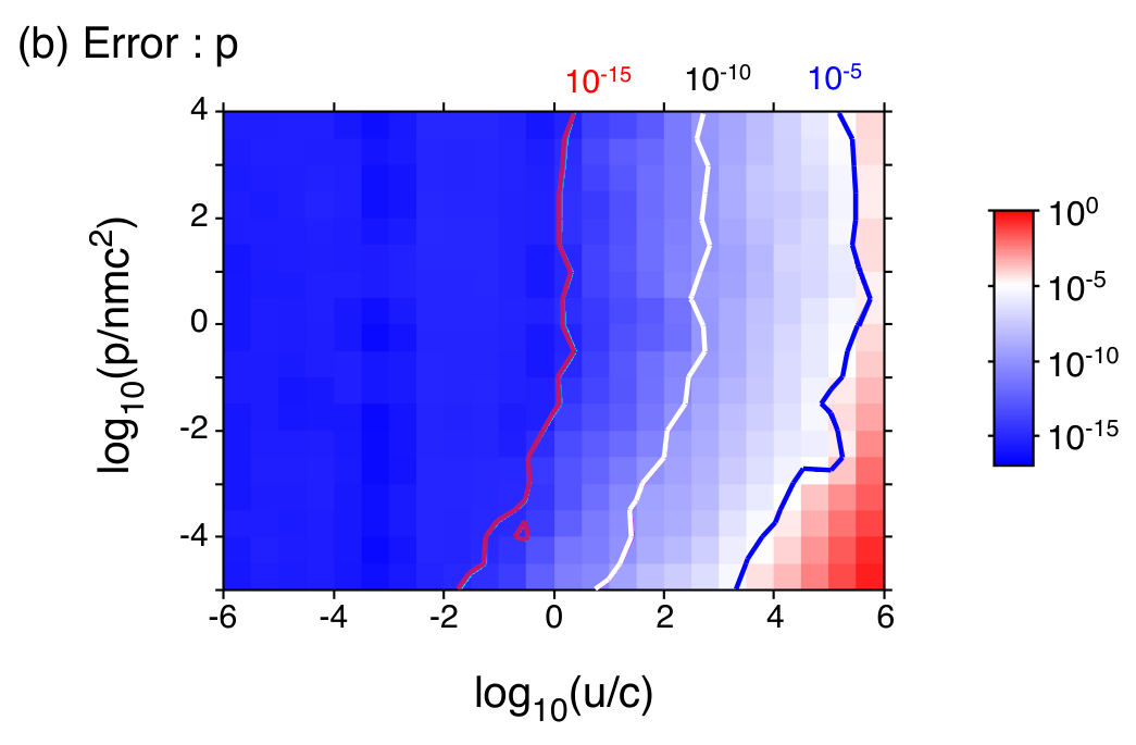
The behavior of our primitive variable solver is characterized by two parameters, the relativistic bulk flow and the relativistic temperature . We benchmarked the numerical accuracy of our solver, and Figure 14 shows the results as a function of the two parameters. We can see that the quartic solution is accurate even in the ultrarelativistic regime of . The pressure is least reliable in the limit of and . This is because the pressure is enclosed in the enthalpy term , but the fluid macro properties are insensitive to in such cases. The error in shows the same trend as that of .

Appendix B Brown Method
We solve the quartic equations by using a simplified version of the Brown method [44]. Consider the following quartic equation:
| (B1) |
where is the th-order coefficient. When we apply eq. A8 to eq. B1, we find that the coefficients are all real, and that . In addition to two solutions (), eq. B1 has one real negative solution () and one real positive solution (). The first two () are usually complex conjugates, and the real positive one is the physically valid solution that we are looking for. Let us consider the following two equations:
| (B2) | |||||
| (B3) |
Examining the properties of and , we know that and that and . Therefore the quartic equation (eq. A8) can be decomposed into two quadratic equations with real coefficients. The relations between , , and are as follows:
| (B4) |
We further define . Using , we rewrite these equations
| (B5) |
We obtain the following relation:
| (B6) |
and then
| (B7) |
We solve this third-order equation to obtain , paying attention to the numerical accuracy [45]. Usually, we obtain two complex solutions and the one real solution in Equation B7, and so we employ the sole real solution . When we find three real solutions in Equation B7, we may have multiple choices for , because Equation B2 also has two real solutions instead of complex conjugates.
By using this , we obtain . Here we choose a positive square root, because we know that . The last variable can be obtained from eq. B5 accordingly. By using , , , and , we obtain and , and then we obtain as a positive root of eq. B3.
If we employed the standard Ferrari’s method to solve the quartic equations, we should use Cardano’s transformation, , in order to eliminate the third-order coefficient . Then, the inverse transformation of often causes the cancellation of significant digits when the solution is very small, . On the other hand, by using Brown method, we are not so influenced by the cancellation of significant digits when the solution is very small, .
References
- [1] M. J. Aschwanden 2006, Physics of the Solar Corona: An Introduction with Problems and Solutions (2nd Edition; Berlin: Springer), Chapter 10
- [2] G. T. Birk, A. R. Crusius-Wätzel and H. Lesch 2001, Astrophys. J. , 559, 96
- [3] N. Bessho and A. Bhattacharjee 2007, Phys. Plasmas , 14, 056503
- [4] E. G. Blackman and G. B. Field 1993, Phys. Rev. Lett. , 71, 3481
- [5] E. G. Blackman and G. B. Field 1994, Phys. Rev. Lett. , 72, 494
- [6] N. Bucciantini, T. A. Thompson, J. Arons, E. Quataert and L. Del Zanna 2006, Monthly Notices of the RAS , 368, 1717
- [7] P. F. Chen and K. Shibata 2000, Astrophys. J. , 545, 524
- [8] R. B. Clare and D. Strottman 1986, Physics Reports, 141, 177
- [9] F. V. Coroniti 1990, Astrophys. J. , 349, 538
- [10] W. Daughton 1999, Phys. Plasmas , 6, 1329
- [11] W. Daughton and H. Karimabadi 2007, Phys. Plasmas , 14, 072303
- [12] L. Del Zanna, N. Bucciantini and P. Londrillo 2003, Astron. Astrophys. 400, 397
- [13] T. di Matteo 1998, Monthly Notices of the RAS , 299, L15
- [14] G. Drenkhahn 2002, Astron. Astrophys. , 387, 714
- [15] G. Drenkhahn and H. C. Spruit 2002, Astron. Astrophys. , 391, 1141
- [16] G. C. Duncan and P. A. Hughes 1994, Astrophys. J. , 436, 119
- [17] R. C. Duncan and C. Thompson 1992, Astrophys. J. , 392, L9
- [18] C. F. Gammie, J. C. McKinney and G. Tóth 2003, Astrophys. J. , 589, 444
- [19] M. Hesse, K. Schindler, J. Birn and M. Kuznetsova 1999, Phys. Plasmas , 6, 1781
- [20] M. Hesse and S. Zenitani 2007, Phys. Plasmas , 14, 112102
- [21] C. H. Jaroschek, R. A. Treumann, H. Lesch and M. Scholer 2004, Phys. Plasmas , 11, 1151
- [22] M. Karlický 2008, Astrophys. J. , 674, 1211
- [23] J. G. Kirk and O. Skjæraasen 2003, Astrophys. J. , 591, 366
- [24] S. Koide and K. Arai 2008, Astrophys. J. , 682, 1124
- [25] S. Koide, K. Nishikawa and R. L. Mutel 1996, Astrophys. J. , 463, L71
- [26] S. Koide, K. Shibata, and T. Kudoh 1999, Astrophys. J. , 525, 727
- [27] S. S. Komissarov 1999, Monthly Notices of the RAS , 303, 343
- [28] S. S. Komissarov 2006, Monthly Notices of the RAS , 367, 19
- [29] S. S. Komissarov 2007, Monthly Notices of the RAS , 382, 995
- [30] H. Lesch and G. T. Birk 1998, ApJ, 499, 167
- [31] Y. Lyubarsky 2003, Monthly Notices of the RAS , 345, 153
- [32] Y. Lyubarsky 2005, Monthly Notices of the RAS , 358, 113
- [33] Y. Lyubarsky and J. G. Kirk 2001, ApJ, 547, 437
- [34] Y. Lyubarsky and M. Liverts 2008, Astrophys. J. , 682, 1436
- [35] M. Lyutikov 2003, Monthly Notices of the RAS , 346, 540
- [36] M. Lyutikov 2006, Monthly Notices of the RAS , 367, 1594
- [37] M. Lyutikov and D. Uzdensky 2003, Astrophys. J. , 589, 893
- [38] J. M. Martí and E. Müller 2003, Living Reviews in Relativity, 6, 7
- [39] F. C. Michel 1982, Rev. Mod. Phys., 54, 1
- [40] F. C. Michel 1994, Astrophys. J. , 431, 397
- [41] A. Mignone, M. Ugliano and G. Bodo, Monthly Notices of the RAS , 393, 1141
- [42] Y. Mizuno, K. I. Nishikawa, S. Koide, P. Hardee, and G. J. Fishman 2006, submitted to ApJS (astro-ph/0609004)
- [43] S. C. Noble, C. F. Gammie, J. C. McKinney and L. Del Zanna 2006, Astrophys. J. , 641, 626
- [44] E. Nunohiro and S. Hirano 2003, Transactions of the Japan Society for Industrial and Applied Mathematics, 13, 159
- [45] E. Nunohiro, M. Suga and S. Hirano 1996, Transactions of the Japan Society for Industrial and Applied Mathematics, 6, 173
- [46] E. N. Parker 1957, J. Geophys. Res. , 62, 509
- [47] H. E. Petschek 1964, “Magnetic Field Annihilation” in AAS/NASA Symposium on the Physics of Solar Flares, W. N. Ness, Ed. (NASA, Washington, DC, 1964), p. 425
- [48] P. L. Pritchett, F. V. Coroniti and V. K. Decyk 1996, J. Geophys. Res. , 101, 27413
- [49] M. Scholer 1989, J. Geophys. Res. , 94, 8805
- [50] A. Spitkovsky 2006, Astrophys. J. , 648, 51
- [51] P. A. Sweet 1958, in IAU Symp. 6, Electromagnetic Phenomena in Cosmical Physics, ed. B. Lehnert (New York: Cambridge Univ. Press), 123
- [52] C. Thompson and R. C. Duncan 1995, Monthly Notices of the RAS , 275, 255
- [53] C. Thompson and R. C. Duncan 2001, Astrophys. J. , 561, 980
- [54] M. Ugai and T. Tsuda 1977, J. Plasma Physics, 17, 337
- [55] N. Watanabe and T. Yokoyama 2006, Astrophys. J. , 647, L123 (WY06)
- [56] P. M. Woods and C. Thompson 2006, in Compact stellar X-ray sources, ed. by W. Lewin & M. van der Klis (Cambridge University Press), 547
- [57] T. Yokoyama and S. Shibata 2001, Astrophys. J. , 549, 1160
- [58] L. M. Zelenyi and V. V. Krasnoselskikh 1979, Astronomicheskii Zhurnal, 56, 819
- [59] S. Zenitani and M. Hesse 2008a, Phys. Plasmas , 15, 022101
- [60] S. Zenitani and M. Hesse 2008b, Astrophys. J. , 684, 1477
- [61] S. Zenitani and M. Hoshino 2001, Astrophys. J. , 562, L63
- [62] S. Zenitani and M. Hoshino 2005a, Astrophys. J. , 618, L111
- [63] S. Zenitani and M. Hoshino 2005b, Phys. Rev. Lett. , 95, 095001
- [64] S. Zenitani and M. Hoshino 2007, Astrophys. J. , 670, 702
- [65] S. Zenitani and M. Hoshino 2008, Astrophys. J. , 677, 531