Stimulus-dependent correlations in threshold-crossing spiking neurons
Abstract
We consider a threshold-crossing spiking process as a simple model for the activity within a population of neurons. Assuming that these neurons are driven by a common fluctuating input with Gaussian statistics, we evaluate the cross-correlation of spike trains in pairs of model neurons with different thresholds. This correlation function tends to be asymmetric in time, indicating a preference for the neuron with the lower threshold to fire before the one with the higher threshold, even if their inputs are identical. The relationship between these results and spike statistics in other models of neural activity are explored. In particular, we compare our model with an integrate-and-fire model in which the membrane voltage resets following each spike. The qualitative properties of spike cross-correlations, emerging from the threshold-crossing model, are similar to those of bursting events in the integrate-and-fire model. This is particularly true for generalized integrate-and-fire models in which spikes tend to occur in bursts as observed, for example, in retinal ganglion cells driven by a rapidly fluctuating visual stimulus. The threshold crossing model thus provides a simple, analytically tractable description of event onsets in these neurons.
1 Introduction
Probing the relationship between a stimulus and the spike train, generated by a population of neurons, is a central theme in the study of neural activity Rieke et al. ((1996)). Correlations in the spike timing of different neurons are of interest, in this context, for two main reasons: First, spike correlations are informative about the structure of the neural code, beyond what could be inferred from the firing properties of single neurons alone. Second, correlations are often thought to reflect the structural properties of the neural network Ginzburg & Sompolinsky ((1994)).
Correlated firing in a pair of neurons can arise because of two distinct reasons: the existence of a connection between the neurons (direct or indirect), and the existence of a common input to the two neurons that is varying in time. Here we focus on the second possible source for correlated activity. We consider model neurons that receive an analog, continuous stimulus, and respond to it by generating a discrete sequence of spiking events. The main question that we address is how the statistical properties of the fluctuating stimulus affect the structure of spike correlation functions.
Correlated inputs to neurons were considered theoretically mainly in context of their effect on single-neuron properties, such as the firing rate Tuckwell ((1988)); Salinas & Sejnowski ((2000)); Moreno et al. ((2002)); Kuhn et al. ((2003)), the coefficient of variation (CV) Tuckwell ((1988)); Brunel & Sergi ((1998)); Salinas & Sejnowski ((2000)); Stroeve & Gielen ((2001)); Salinas & Sejnowski ((2002)); Schwalger & Schimansky-Geier ((2008)), and the spike-triggered average stimulus Kanev et al. ((2003)); L. et al. ((2006)); Paninski ((2006)). These works considered integrate-and-fire model neurons Tuckwell ((1988)); Gerstner & Kistler ((2002)).
The non-leaky integrate-and-fire model is relatively tractable analytically Tuckwell ((1988)); Paninski ((2006)). In comparison, analytical treatment of the leaky integrate-and-fire (LIF) neuron is considerably more difficult Burkitt ((2006)). Some analytical results are available for the firing rate Salinas & Sejnowski ((2000)); Moreno et al. ((2002)); Kuhn et al. ((2003)), whereas analytical results for the ISI and the CV are available only in particular limits such as slowly varying Moreno-Bote & Parga ((2006)); Schwalger & Schimansky-Geier ((2008)), or binary Salinas & Sejnowski ((2002)), inputs. Other results were obtained for the LIF model from computer simulations Salinas & Sejnowski ((2000)); Stroeve & Gielen ((2001)). In particular, Stroeve & Gielen ((2001)) included a simulation study of correlations in spiking of LIF neurons that receive partly overlapping input. Correlations due to partly overlapping input were also studied analytically, but only in the limit where the input is slowly fluctuating in time Moreno-Bote & Parga ((2006)).
Here we consider a simpler model of neural response, where neurons spike whenever a generating potential , linearly related to the neuron’s stimulus, crosses a threshold in its rising phase. For sufficiently simple stimuli this model is analytically tractable, which allows for spike correlation functions to be evaluated in closed form.
Threshold crossing processes without a reset were previously analyzed as models for neural firing. The spike auto-correlation function of a neuron was considered by Jung ((1994)), while making specific assumptions on the nature of the fluctuating potential. Here we evaluate the auto- and cross-correlation in spike timing of neurons with different thresholds, while making fewer assumptions on the generating potentials eliciting the spikes. These are assumed to be Gaussian, and may be identical or partially overlapping in different neurons.
As in the case of Linear-Nonlinear (LN) models Korenberg & Hunter ((1986)); E. Chichilnisky ((2001)), we assume that a neuron responds to a temporal convolution of its stimulus with a linear kernel. However, in the LN model spiking is stochastic, whereas in the threshold-crossing model the spike timing is precisely determined by the stimulus. This aspect of the model is motivated by the observation, in various neural assays, of responses that are precisely repeatable across multiple trials Mainen & Sejnowski ((1995)); Berry et al. ((1997)); R.R. de Ruyter van Steveninck et al. ((1997)); Meister & Berry ((1999)); Keat et al. ((2001)); Uzzell & Chichilnisky ((2004)), much more than can be described by Poisson statistics, particularly when the stimulus is strongly fluctuating in time.
The model and our main assumptions are presented in Sec. II. Before discussing spike correlation functions, we first evaluate the firing rate (Sec. III), the spike-triggered average stimulus, and the spike-triggered covariance (Sec. IV). We then evaluate spike auto- and cross-correlation functions (Sec. V). These results are compared with computer simulations of model neurons that spike according to several variations of the leaky integrate-and-fire model (Sec. VI).
2 Formalism and assumptions
We consider one or more neurons that respond to the same generating potential and elicit a spike whenever crosses a threshold in its rising phase. The spike train generated by the neuron can be written as
| (1) |
where is the generating potential. The Heaviside step function restricts the firing to the upward crossing events.
We assume that is stationary, Gaussian, and has zero mean. The generating potential is thus fully characterized by its correlation function,
| (2) |
where the brackets stand for an ensemble average over all possible realizations of the fluctuating generating potential . Later on, in Sec. V, we consider a more general situation of a population of neurons, whose generating potentials are jointly Gaussian, characterized by their covariance functions
| (3) |
The properties of a model neuron, responding to a stimulus whose mean differs from zero, can be obtained from the zero-mean case simply by adjusting the threshold.
For a single neuron, the behavior of at small determines the firing rate and the short-time behavior of the spike auto-correlation (Sec. V). We assume that an expansion of exists around ,
| (4) |
We further assume that vanishes and that is negative, for reasons that will become clear later on. As seen below, it is necessary to treat separately different classes of processes, depending on which other coefficients in the expansion are non-zero. One important class is the case where . This is the typical situation if a causal filter is involved in the generation of . For comparison we also briefly consider, in Sec. V, the case where all the coefficients with odd indices vanish; for example, a process with a Gaussian correlation function, .
Relationship between and the stimulus
The generating potential in our model is linearly related to the stimulus ,
| (5) |
where the symbol ‘’ stands for convolution. We assume that is a zero-mean, uncorrelated Gaussian process:
| (6) |
The correlation function of is then
| (7) |
Note that and that if is sufficiently regular, .
The assumption that is uncorrelated is made for simplicity of the presentation, and because uncorrelated flickering stimuli are often used experimentally. The results below generalize in a straightforward manner also to the case where is a correlated Gaussian process.
Specific forms for and
In the following sections we first derive results that are valid generally, for any . We then illustrate these results with a specific example, where we assume a particular form of . In these examples the filter is a causal filter of the form
| (8) |
which is a combination of two single-exponential filters with time constants and . Using Eq. (7)
| (9) |
where
| (10) |
is the variance of .
In the particular case where , is an ‘alpha’ filter,
| (11) |
and
| (12) |
The expansion of for small , Eq. (4), yields and:
| (13) |
3 Firing rate
We begin with the relatively simple problem of evaluating the firing rate of a single neuron Rice ((1954)),
| (14) |
where is given by Eq. (1). Although this quantity has been calculated before, we derive it here in some detail, because the derivation generalizes to the higher-order moments that are calculated later (whose detailed derivation is presented in the appendices.) The firing rate can be written as
| (15) |
where is the joint probability distribution for the generating potential to be equal to and for its derivative, at the same time, to be equal to . To evaluate this and similar quantities, we use an identity that holds for a general Gaussian signal with correlation function : If are all scalar random variables that depend linearly on the process ,
| (16) |
then the joint probability distribution of is equal to
| (17) |
where and
| (18) |
The generating potential and its derivative at time correspond to and , therefore and , so that
| (19) |
The off-diagonal terms are proportional to , which vanishes if , as we assumed11 1 If , does not have a derivative at , and the derivation performed here fails. A typical example is given by uncorrelated noise passed through a single-exponential filter. For this process the firing rate diverges (see below).. We thus have
| (20) |
and the integral (15) yields
| (21) |
Hence must be negative for the firing rate to be finite.
For the generating potential of Eqs. (8) and (9),
| (22) |
If either or vanish, the firing rate diverges. Hence a generating potential obtained by convolving uncorrelated noise with a single exponential filter has an infinite rate of threshold crossings. In such a process there are finite intervals in which the number of crossings is infinite, and others in which no firing occurs22 2 This is related to the short-time properties of the spike auto-correlation function (Sec. V) in the limit where or ..
4 Spike triggered average stimulus
The spike triggered averaged stimulus (STA) is the mean stimulus given that a spike was generated at a particular time. Because the input is assumed to be stationary, the STA is only a function of the time difference relative to the spike time,
| (23) |
where is the firing rate, is determined by , as in Eq. (1), and the spike time was arbitrarily chosen to be zero. If one assumes that spiking is described by a LN model with filter , and if the stimulus is uncorrelated Gaussian noise, is proportional to E. Chichilnisky ((2001)); Paninski ((2003)). Hence it is common to probe the spatio-temporal filter applied by a neuron on its stimulus by measuring Schwartz ((2006)), in particular in the visual sensory system Rieke ((2001)); E.J. Chichilnisky & Kalmar ((2002)); Baccus & Meister ((2002)); Rust et al. ((2005)); Hosoya et al. ((2005)).
To compute for a threshold-crossing spiking neuron we need the joint probability distribution function for , , and , evaluated in Appendix A. The STA is then given by
| (24) |
where and .
The first term in Eq. (24) is proportional to the expectation for the STA in a rate-based linear-nonlinear model E. Chichilnisky ((2001)). However, for a threshold-crossing spiking neuron it correctly describes the STA only in the limit of large : in contrast, when , the STA is proportional to .
The result that is a linear combination of the filter and its derivative has a simple geometric interpretation, which is most easily seen by thinking of the stimulus history as an -dimensional discrete vector. The condition for spiking at time involves and its derivative, which are the inner products of the stimulus history with two vectors, and . Because is uncorrelated, its history vector is distributed in a radially symmetric manner in -dimensional space. The STA must lie in the two-dimensional sub-space spanned by the vectors and .
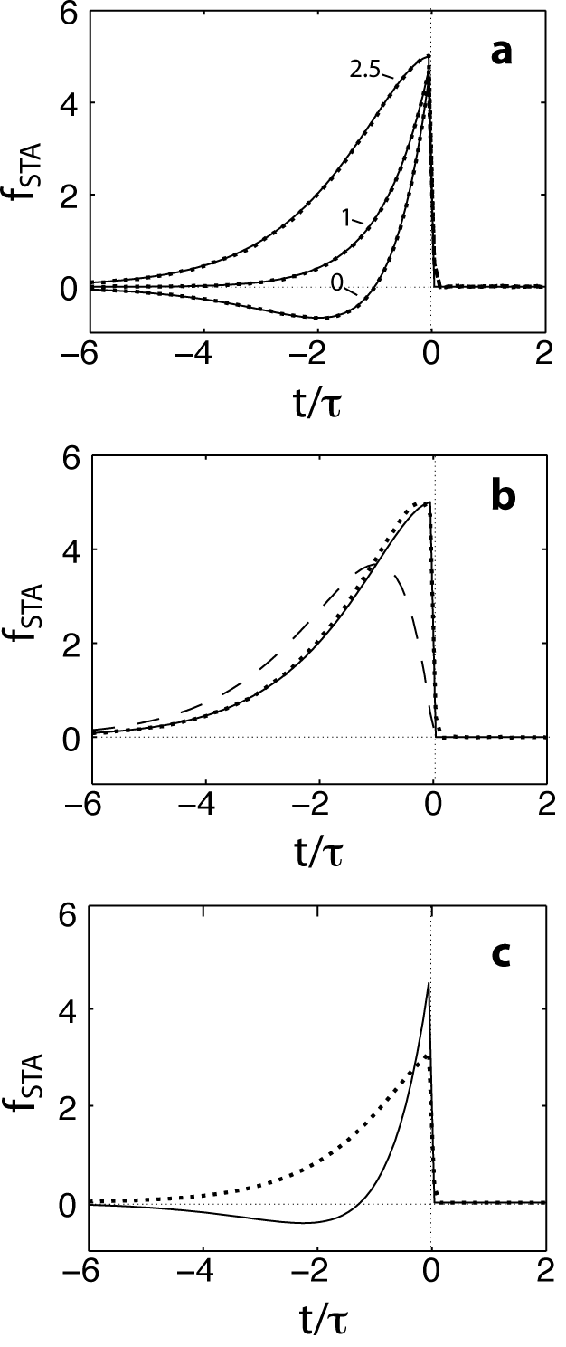
This result is illustrated in Fig. 1a, for the generating potential of Eqs. (11) and (12). With the threshold varying from 0 to , the shape of varies significantly. The dotted lines in the figure (overlapping with the solid line) were obtained from a discrete simulation, using a time step and averaging over a simulation run for and , and for .
It is interesting to compare these results with what is expected from a leaky integrate-and-fire model neuron Tuckwell ((1988)); Gerstner & Kistler ((2002)). For this case there is no known analytic form for the STA (see, however, Kanev et al., (2003); L. et al., (2006); Paninski, (2006)), but we can evaluate the STA numerically. We assume that the membrane potential of the model neuron is related to the input current via
| (25) |
with a reset of the membrane potential to whenever reaches the threshold , whereas the input current is related to the stimulus by
| (26) |
The sub-threshold dynamics of depends on the stimulus in the same way as the generating potential depends on stimulus in the threshold-crossing model. The difference between the two models lies in the existence of a reset. For simplicity, we set and for the rest of this section (see also Sec. 6 and Appendix D).
Figure 1b shows a comparison between in the integrate-and-fire model (simulation, dotted line: and ) and in the threshold-crossing spiking model [Eq. (24), solid line.] The parameters are as in panel a, with a threshold . The two models agree very well in their prediction and differ, significantly, from that of a LN model, where (dashed line).
For a lower threshold, , the threshold-crossing spiking model and the integrate-and-fire model no longer yield similar predictions for (solid and dashed lines, Fig. 1c). The difference between the cases of high and low threshold is possibly related to the typical inter-spike interval which, in the case of a high threshold, is longer, allowing the input to decorrelate between subsequent spikes. The statistics of the input before a spike are thus less influenced, in the case of high threshold, by whether a reset has occurred following the previous spike.
Finally, we note that the threshold-crossing model is similar to a two-dimensional LN model involving two filters, equal to and . In the analogous LN model the nonlinear transfer function must be chosen to be narrowly peaked at values of the generating potential close to the threshold, and an appropriate dependence on the derivative must be included as well33 3 There is a difference between the two models, however, in that the two-dimensional LN model produces a variable number of spikes within the narrow spiking event.. The result that the STA is a linear combination of the filter and its derivative thus agrees with the general property of multi-dimensional LN models, that the STA lies within the subspace spanned by the linear kernels determining the spiking rate Paninski ((2003)); Schwartz ((2006)). Similarly, we may expect the spike-triggered covariance R. de Ruyter van Steveninck & Bialek ((1988)); Schwartz ((2006)) to reveal the linear filter and its derivative as spanning this sub-space. This is indeed the case (Appendix A.)
5 Spike correlations
We next consider correlations in the spike timing of two neurons, assuming that they receive identical inputs, but possibly differ in their thresholds . Because the generating potential is assumed to be stationary, the spike correlation function depends only on the time difference between spikes:
| (27) |
From the definition of , Eq. (1), the quantity inside the brackets depends on the generating potential and its derivative at and at .
The detailed form of is derived in appendix B, and here we present the main results. The spike correlation function can be written as
| (28) | |||||
where is the joint probability distribution for and [see Eq. (66)], and . The quantity in the second line of the equation is the conditional probability distribution function for and , given that and . This conditional distribution is Gaussian and is characterized by its mean and the covariance matrix , whose values are derived in the appendix [Eqs. (64) and (65)].
The spike auto-correlation function
We briefly discuss the spike auto-correlation function, corresponding to the case , and focusing on the behavior at small . Because the spike train is a point process, its auto-correlation function necessarily includes a contribution
| (29) |
The discussion here concerns nonzero values of , i.e., the occurrence of spikes in addition to the one at . The behavior for small is remarkably different for the two classes of generating-potential statistics discussed in Sec. II: If , as in the example of Eq. (13), the spike auto-correlation function tends to a finite value when :
| (30) |
It is interesting to look at this quantity divided by , which represents the firing rate at time after the occurrence of a spike at :
| (31) |
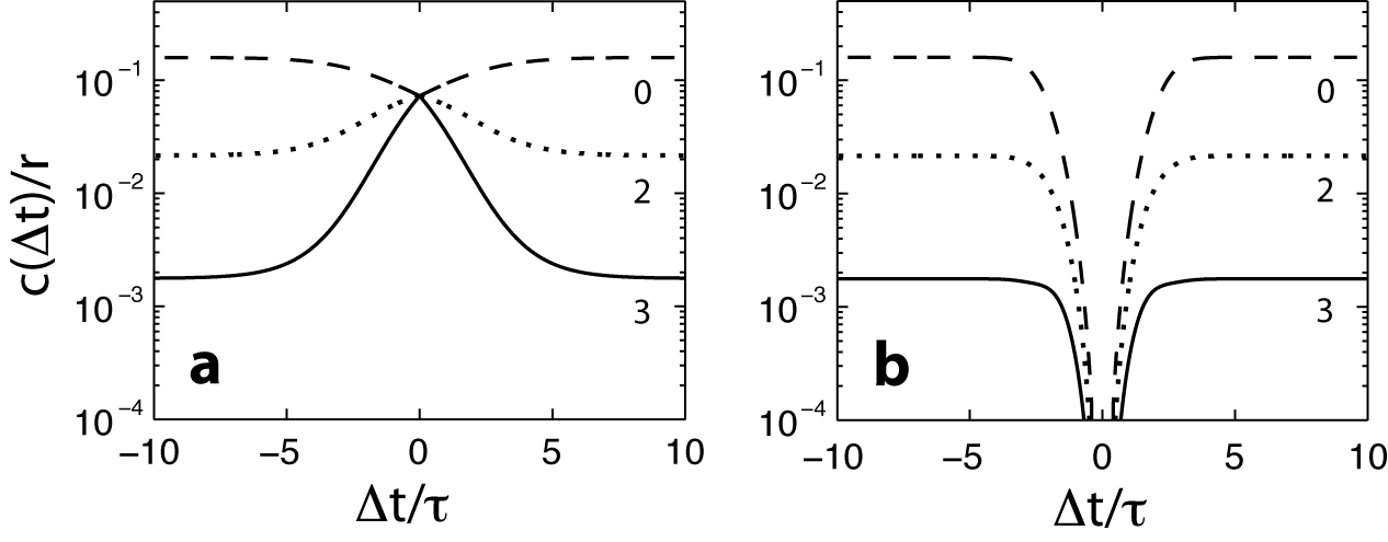
This ratio does not depend on . By comparing with itself we see that, if the threshold is high, the spike-conditioned firing rate is much higher than the average firing rate. In other words, once the neuron has fired, it is likely to soon fire again, compared to its baseline firing rate. When the threshold is zero, the spike-conditioned firing rate can be larger or smaller than , depending on the expansion coefficients and . This result is illustrated in Fig. 2a, where is given by Eq. (12)44 4 Note that the conditional firing rate diverges if or if , which can be seen from Eq. (13). This is consistent with the divergence of the average firing rate in this limit, and the existence of finite time intervals in which the number of spikes is infinite..
We note that when as above, the second derivative of the generating potential is an unbounded random process, and the first derivative of is not smooth. This facilitates the generation of successive spikes at short intervals, since the derivative of is required to be positive at the interval’s edges, and negative somewhere in between.
In contrast, when the first derivative of is a smooth process, we may expect the occurrence of spikes at vanishingly small intervals to be considerably less likely. Indeed, if has no irregularities at , so that all with odd indices vanish, the occurrence of spikes separated by short intervals is strongly suppressed, [Appendix C, Eqs. (84) and (87)]. This is illustrated in Fig. 2b for a generating potential with a Gaussian correlation function, . Note that and are the same in the two parts of Fig. 2; consequently, the mean firing rates are identical in these two cases.
Spike cross-correlation
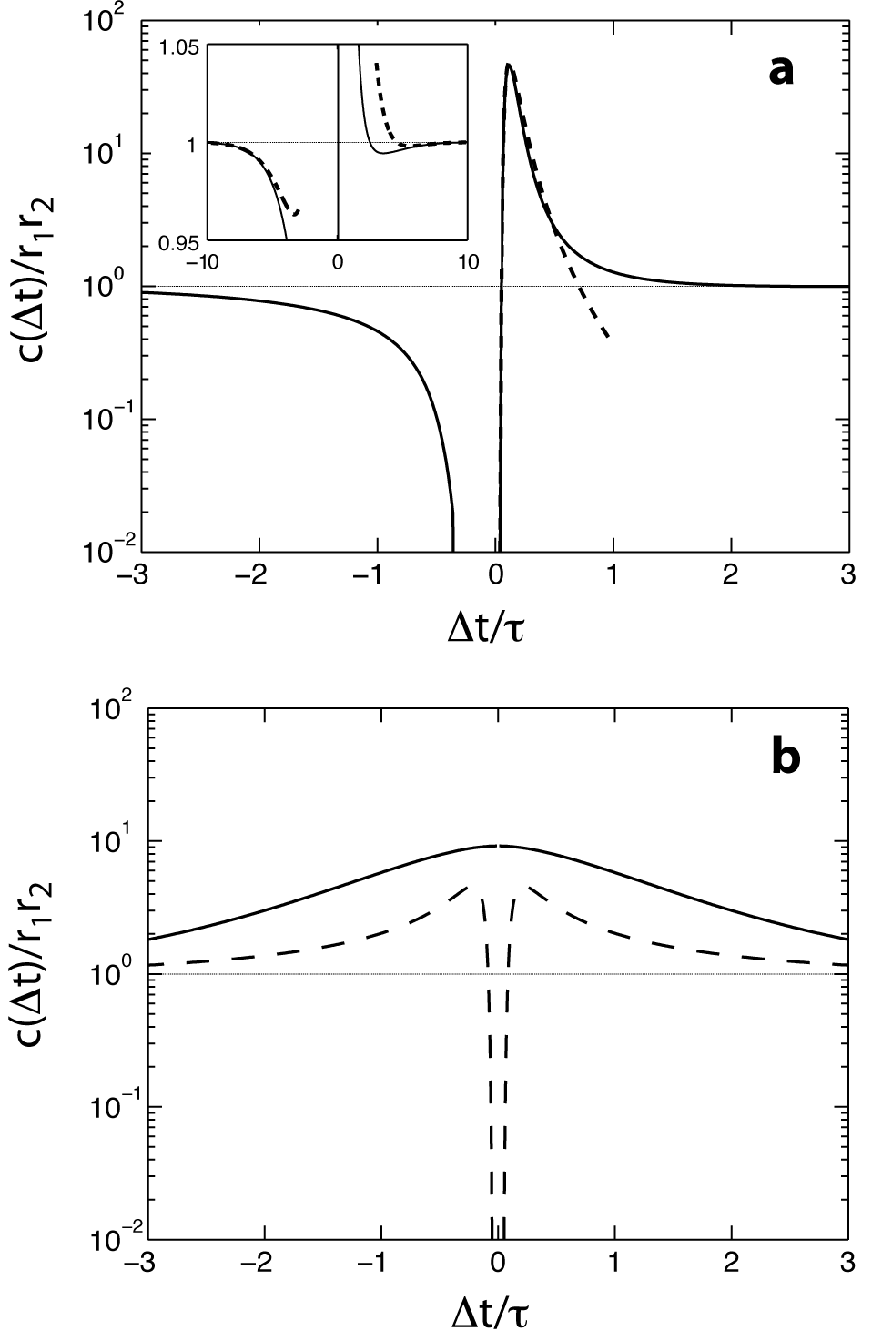
We next consider the spike cross-correlation function of two neurons with different thresholds, firing in response to the same stimulus. We note, first, that unless the correlation function is not symmetric with respect to replacement of by or, equivalently, with respect to exchange of the two neurons (). The generating potential is required to have a positive derivative at and at , and therefore we may expect a higher probability for joint spiking if the higher of the two thresholds is set at the later time (see Fig. 3). This is indeed the case – as demonstrated in Fig. 4a for the generating potential described by Eq. (12), and with thresholds set as and . The preference for one neuron to fire after the other neuron is particularly prominent at short time scales of order , but it also has a signature at large time scales (Appendix B).
It is instructive to compare the threshold-crossing model with the prediction of a one-dimensional linear-nonlinear (LN) model E. Chichilnisky ((2001)). For this comparison, we assume that the linear filter of the LN model is the same as the filter in the threshold-crossing model, and that in both models the stimulus is uncorrelated Gaussian noise. In the LN model the spike correlation function depends also on the choice of the non-linear function applied to the outcome of the linear filter. Two particular choices are made in the examples shown in Fig. 4b: The first is linear rectification, where for and for , with thresholds chosen as in Fig. 1a (solid line).
The second example (dashed line) is the case where is non-zero only in a narrow range around , . Mathematically, this example compares more directly with the threshold-crossing model, because the LN model produces spikes only at the threshold crossings. The correspondence can be seen in the spike cross-correlation function obtained from the LN model in this case, which is calculated in Appendix E [Eq. (100).] In the limit of large , in the LN model [Eq. (104)] is equal to the first term in the large expansion for the threshold-crossing model, Eq. (74).
We note two important qualitative differences between the LN model and the threshold-crossing spiking model: First, in the LN model, the spike correlation function is symmetric under time reversal: 55 5 This property arises for the following reason. The spike cross-correlation at any two times depends on the joint probability distribution of the generating potential values at these times. Assuming that the generating potential is Gaussian, this joint distribution function is necessarily symmetric.. A second qualitative difference between the two models, seen in Fig. 4, is that the firing of the two neurons is less correlated in the LN model, compared to the threshold crossing spiking model, at short time scales.
The limit
In the limit of small the behavior of is substantially different if the neuron with the higher threshold fires before or after the neuron with the lower threshold66 6 A weak asymmetry between positive and negative exists also in the limit . This limit is considered in Appendix B.. To simplify notation we assume here that .
: For small the spike correlation function scales with as
| (32) |
where
| (33) |
This approximation, with the appropriate prefactors taken from Eqs. (60), (76), and (78) is plotted in Fig. 4a (dashed line) for the particular input considered in this figure.
As , the exponential decay in Eq. (32) wins over the divergence for sufficiently small . At larger values of the spike correlation function peaks, and then decays algebraically. Hence the neuron with the larger threshold tends to fire after the neuron with the lower threshold, with a typical latency given by the position of the peak. If we ignore the term , which is legitimate when the difference in thresholds is sufficiently small, the maximum is at where
| (34) |
For the generating potential of Eqs. (8) and (9),
| (35) |
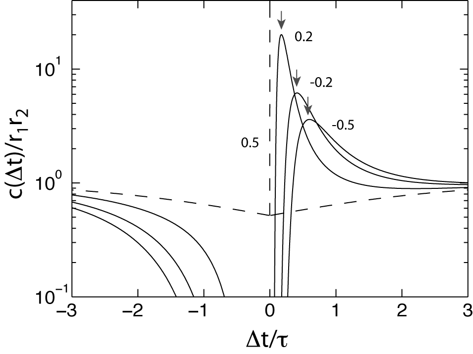
Equation (34) indicates that the most likely latency increases linearly with . An illustration of this result is shown in Fig. 5, where and are as defined by Eqs. (11) and (12), , and is plotted for three values of : , , and (solid lines). With increase in the peak of the spike correlation function becomes wider, and occurs at larger latencies. The arrows indicate the prediction for the position of the peak, Eq. (35), which matches the actual position very well even when is relatively large.
: In this case the process is required to have a positive derivative at , a negative derivative within the interval and, again, a positive derivative at . Such a trajectory becomes increasingly unlikely when , and the spike correlation function decays to zero. The leading contribution is of the form
| (36) |
if . If the decay is even stronger, (Appendix C.) Equation (36) introduces a characteristic time scale for the inhibition, scaling as
| (37) |
where the expression on the right hand side holds if is given by Eq. (9).
Partly overlapping inputs
We next generalize the analysis to the more realistic case where the inputs to different neurons are only partially overlapping:
| (38) |
The noise inputs are assumed to be zero-mean, jointly Gaussian processes that are uncorrelated with and with each other:
| (39) |
Here is the ratio between the standard deviation of the noise and that of the common stimulus. The covariance of the generating potentials is then
| (40) |
The spike auto- and cross-correlation functions can be evaluated in a similar manner as for the noise-free case (Appendix B).
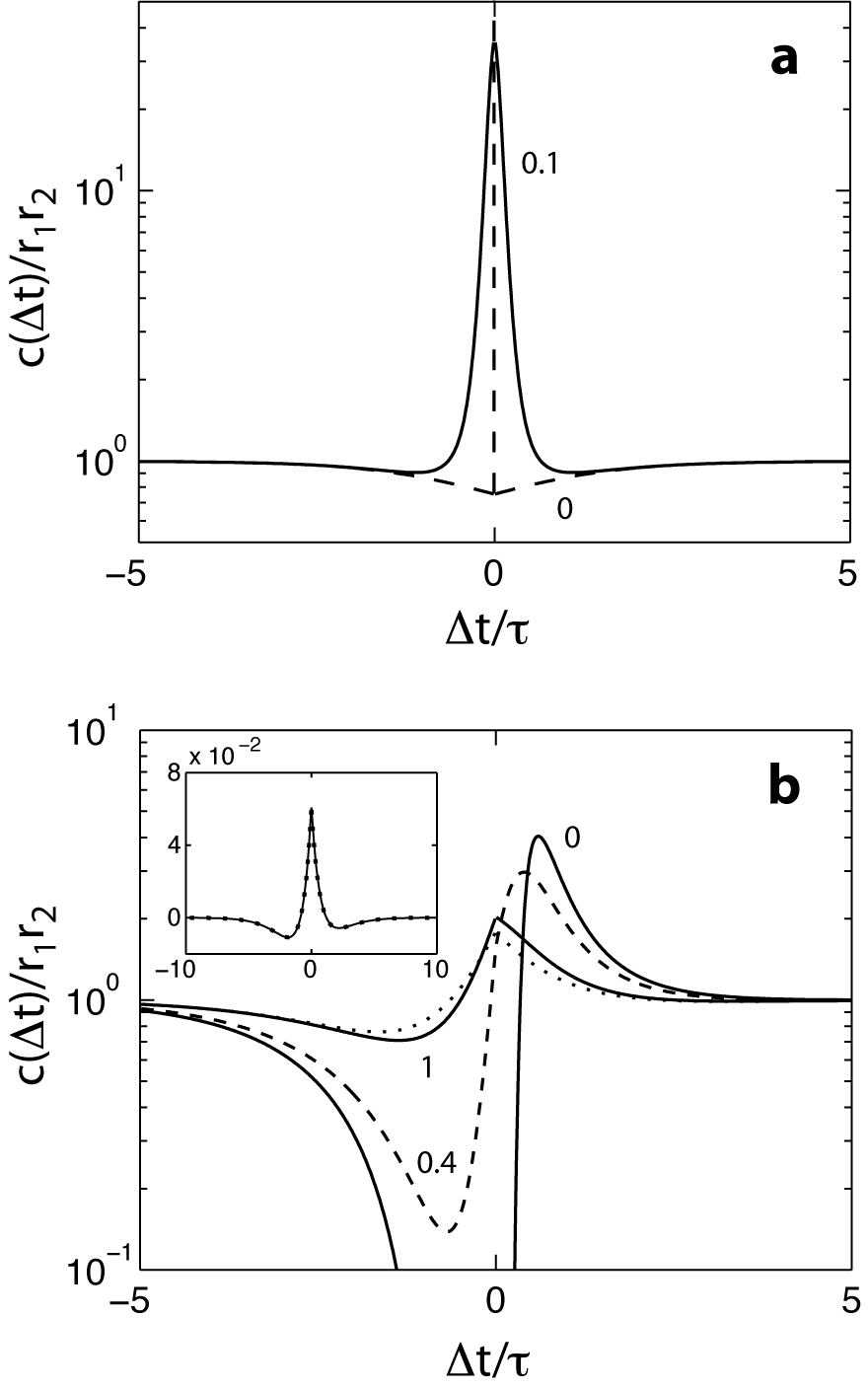
As an example, we consider the ‘alpha’ filter, Eq. (11). In Fig. 6 the standard deviation of the common stimulus is kept fixed, while is varied. Figure 6a shows the spike correlation function of two model neurons with the same threshold and with weak independent noise, . The existence of noise increases the correlation in neural firing at non-zero latencies, compared to the noise-free case (dashed line). To understand this seemingly counter-intuitive result, note that the spike correlation function in the noise-free case is identical to the spike auto-correlation function of a single neuron, and includes a delta-function contribution at . When the two neurons receive independent noise, they no longer fire precisely a the same time, leading to a broadening of the delta function into a peak of finite width.
Panel b of the figure shows the spike correlation function of two neurons with different thresholds, and , for several values of : 0 (no noise), 0.4, and 1. Increasing reduces the correlation between the two neurons. Note, however, that the preference of neuron to fire after neuron 1 is clearly evident at time scales comparable to , even when the noise and signal have the same standard deviation.
The inset shows in a case where the noise is much larger than the signal, . Here is very well approximated using a linearization with respect to the cross-correlation function (dotted line), as described in Appendix B, Eq. (63). This approximation works quite well even if is of order unity, as can be seen in the main plot (Fig. 6b, dotted line.)
6 Comparison with integrate-and-fire neurons
Having characterized the spike correlation statistics of the threshold crossing model, we may ask whether the results carry over to other models of neural firing. In even the most simple leaky integrate-and-fire (LIF) model an analytical form is not known for the spike correlation functions. Hence the discussion in this section is based on numerical simulation of model neurons, using several variations of the LIF model. We focus on the relative timing of spikes elicited by neurons that receive the same stimulus but differ in their thresholds.
In the following examples, where we consider pairs of neurons that differ in , we suppose that the neurons are identical, but differ in the mean value of their fluctuating input currents. Hence, after shifting the membrane potential to compensate for the different baseline currents, the reset potentials in the two neurons differ, but the difference is fixed.
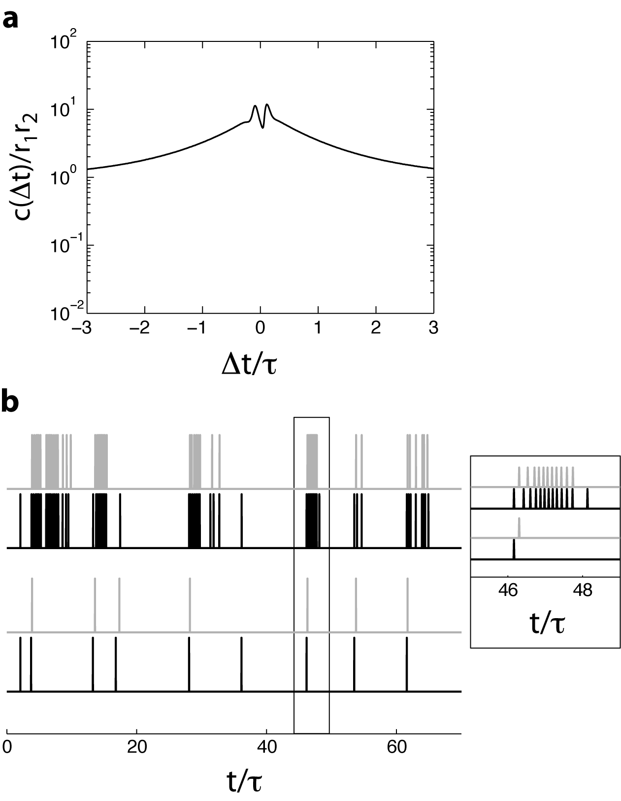
Figure 7 a shows the spike correlation function of two such neurons, evaluated from simulation of model neurons according to the LIF model of Eqs. (25)–(26), with , , and . The only difference between the LIF model and the threshold-crossing model is the existence of a reset in the membrane potential following each spike. Nevertheless, comparing Fig. 7 a with Fig. 4 a reveals that there is very little resemblance between the spike correlation functions obtained from the two models. Most notably, in the LIF model there is almost no preference for one of the neurons to fire later than the other one.
To better understand this discrepancy, Fig. 7 b shows an example of spike trains generated by the two neurons in the LIF model (top two traces), and in the threshold crossing model (bottom two traces). Compared to the LIF model, which tends to produce bursts of spikes, the threshold crossing model tends to generate much more isolated spikes.
The inset in Fig. 7 b shows an example of bursts of spikes, generated by the LIF neurons after a relatively long silent period (top two traces). The first spike generated by the neuron with the smaller threshold (black) precedes the first spike generated by the neuron with the higher threshold (gray), preserving the tendency that is observed in the threshold crossing model. This tendency is typically observed also in other isolated bursts.
Within the bursts, however, there is no clear relative timing of spikes of the two LIF neurons, because a spike in one neuron can be paired with a spike in the other neuron that either precedes it or comes after it. This suggests that the existence of bursts masks the tendency of the neurons to fire in a particular order. Motivated by these observations, we consider several situations in which the LIF model can exhibit a characteristic order of spike timing, in similarity to the prediction of the threshold-crossing model.
Sparse firing
In situations where the LIF neurons fire isolated spikes, we may expect a clear order of spike timing to emerge, and to be reflected in the spike correlation function.
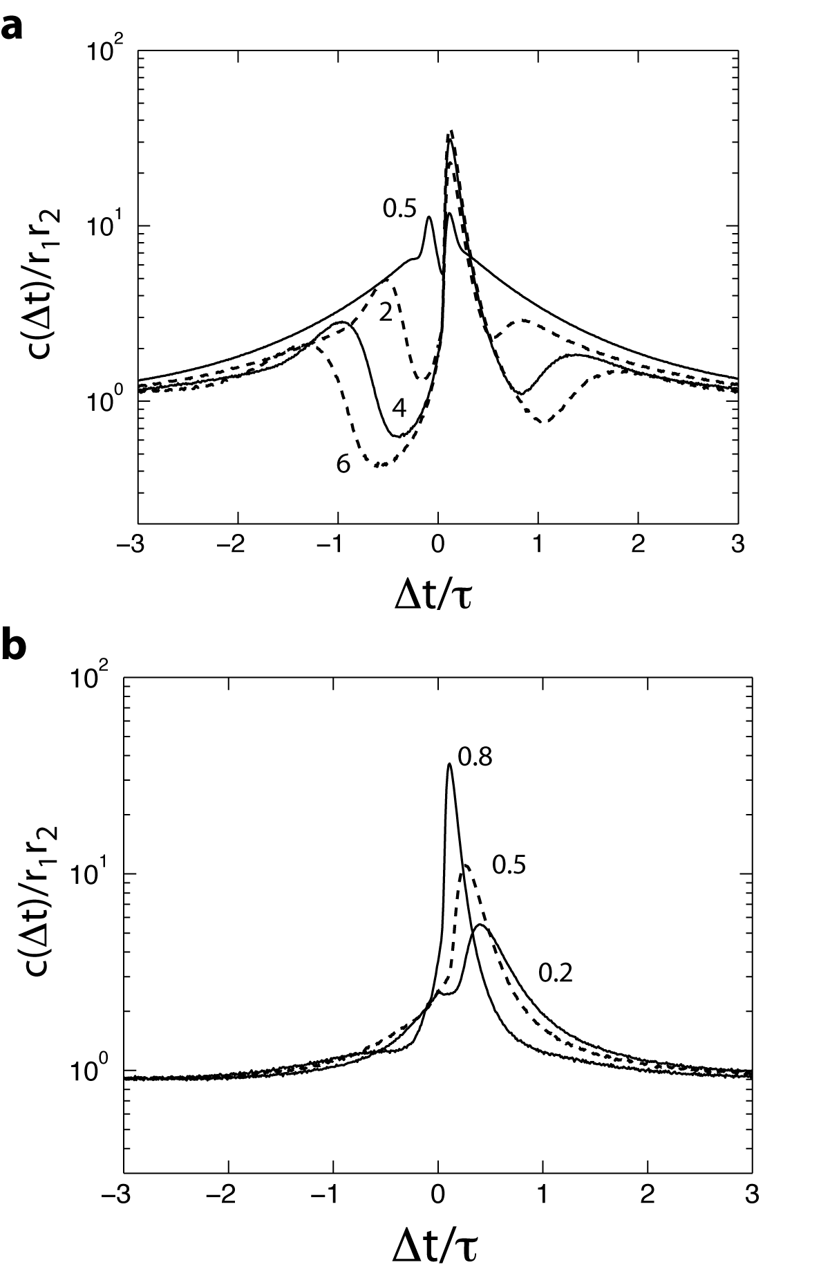
Sparse firing due to a large potential reset, compared to the input variance. With increase of , compared to , spikes tend to become more isolated. With fixed biophysical parameters of the cell, an increase in corresponds to a decrease in the standard deviation of the fluctuating input current (see, also, Appendix D). Figure 8 a shows that, as increases in both neurons, a pronounced asymmetry develops in their spike cross-correlation function.
Sparse firing due to refractoriness. Sparse firing may result, alternatively, from the existence of an additional refractory mechanism. There are many possible ways to model refractoriness in a LIF model Gerstner & Kistler ((2002)), and here we consider one such possibility. After each spike, the membrane potential is kept fixed at during a waiting period whose length varies randomly from spike to spike. After the waiting period the membrane potential continues to evolve according to Eq. (25), and the distribution function of waiting times decays exponentially with a time constant . Spike correlation functions, obtained from simulations of this model with , are shown in Fig. 8 b for several pairs of thresholds, exhibiting a clear asymmetry in firing order. Note that in this example, the membrane time constant is shorter than the typical refractory time .
Bursting events
Neurons often generate distinct bursts of spikes, sometimes referred to as events, when presented with stimuli possessing rapid temporal fluctuations Berry et al. ((1997)); Berry & Meister ((1998)); Berry & Meister ((1998)). It has been argued that the timing of events, as marked by their first spike, can convey significant information about the stimulus Hopfield ((1995)); Gollisch & Meister ((2008)). Hence it is of interest to understand the factors influencing the relative timing of these spikes. In the following, we consider a model where bursting events are more clearly separated from each other than in the simple LIF model. We then interpret the predictions of the threshold-crossing model in relation to the timing of burst onsets.
To reproduce well-separated spiking bursts in a neural model, we consider a generalization of the LIF model, introduced by Keat et al. ((2001)). This model was shown to reliably predict the structure of spike trains generated by retinal ganglion cells from several different species, in response to rapidly flickering stimuli. In a version of this model without noise, a generating potential is related to the stimulus by Eq. (5), as in the threshold crossing model. Spiking occurs when crosses a time-dependent threshold that increases following each spike,
| (41) |
We refer to this model as the variable-threshold (VT) model.
We may interpret as the neuron’s membrane potential: with this interpretation the discrete increase in following a spike corresponds to a reset of the membrane potential from to . The VT model is precisely equivalent to the LIF model of equations (25)–(26) if is a double exponential filter, as in Eq. (8), and if . For simplicity we take to be an ‘alpha’ filter, Eq. (11). However, we choose the time scale of threshold recovery to be larger than the neuron’s membrane time constant, . This ratio roughly matches the relation between and the shape of filters that were found in Keat et al. ((2001)) to provide a good description of spike trains from retinal ganglion cells.
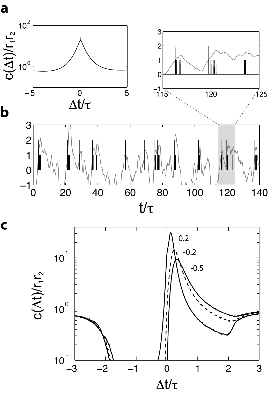
A spike train generated by this model is shown in Fig. 9b, and consists of clearly separated events. The red lines in Fig. 9 b represent spikes generated by a threshold-crossing model with the same generating potential and threshold as in the VT model. These spikes roughly match the onset of busting events in the VT model. The threshold-crossing model thus provides a coarse-grained description of events generated by the VT model.
We next isolate the first spikes of events in the VT model by discarding any spike that occurred within a time delay from a previous spike77 7 Because the events are clearly separated clearly from each other, the results are insensitive to the precise choice of .. Fig 9 c shows the cross-correlation function of these specifically selected spikes in several neurons with thresholds , , , and , that were all presented with the same stimulus. These cross-correlation functions display a strong asymmetry between positive and negative , and are qualitatively very similar to the spike cross correlations in the threshold crossing model, shown in Fig. 5. In contrast the spike cross correlation functions calculated directly from all the spikes, Fig. 9 a, are very different from the prediction of the threshold-crossing model.
These results suggest that the onsets of bursting events in neurons that receive the same stimulus, but differ in their threshold, can exhibit strong asymmetry in their relative timing, and that the correlation functions of these event onsets can be qualitatively described by the simplified threshold-crossing model.
7 Summary
We considered in this work a relatively simple deterministic process that produces a discrete spike train from an analog, continuous signal. The timing of spikes in this model is more precisely controlled by the stimulus than typically predicted by rate-based models. This aspect of the model is motivated by observations of precisely timed spiking in neural assays, particularly in response to stimuli that possess strong temporal modulations Mainen & Sejnowski ((1995)); Berry et al. ((1997)); R.R. de Ruyter van Steveninck et al. ((1997)); Meister & Berry ((1999)); Uzzell & Chichilnisky ((2004)). Some of the salient properties of spike correlation functions in this model are summarized below.
Most notably, two neurons receiving identical inputs can show a preference for one neuron to fire later than the other, although there is no monosynaptic connectivity between them (Figs. 4a and 5.) This preference is prominent even if the thresholds of the two neurons are similar (but not equal), and if there is only partial overlap in their input (Fig. 6.)
Comparison with the leaky integrate-and-fire model shows that bursting in LIF neurons often masks the preference of neurons to fire in a particular order (Fig. 7). However, there are several situations in which such a preference may be observed in LIF neurons. First, LIF neurons can display a preference to fire in a particular order if they produce sparse spiking, e.g., due to a large hyperpolarizing step in the membrane potential after each spike, compared to the standard deviation of the stimulus, or due to other sources of refractoriness (Fig. 8). Second, when the neurons generate clearly separated bursting events, the first spikes of these events have cross-correlation functions that are similar to those predicted by the threshold crossing model (Fig. 9).
The spike cross-correlation function of neurons that differ only in their thresholds may be probed experimentally by repeatedly presenting the same stimulus to a single neuron, while injecting varying amounts of current into the neuron from trial to trial. Correlations between different trials can then effectively measure the spike correlation function of two identical neurons with different thresholds. This approach was recently taken in Markowitz et al. ((2008)), where a Gaussian stimulus, mimicking the spectral properties of Gamma oscillations, was injected into rat pyramidal neurons from the somatosensory cortex. While spike cross-correlation functions are not shown in Markowitz et al. ((2008)), spike trains from different trials exhibit a clear modulation of spike timing by the varying injected current, suggesting that a strong asymmetry exists in the spike-correlation function of neurons with different thresholds. Furthermore, the characteristic latency between the firing of two neurons appears to increase linearly as a function of the difference in injected currents. This roughly linear dependence persists over a wide range of current differences, in similarity to our results from the threshold-crossing model.
We also considered in this work the spike-triggered average stimulus (STA). The STA in our model is a linear combination of the filter and its derivative. A simple geometrical argument shows that this result extends to a larger class of models: it should hold whenever the stimulus is passed through a linear kernel, if spike decisions are then based strictly on the output of the kernel and its derivative. Varying the threshold modifies the relative weight of the filter and its derivative (Fig 1). It will be interesting to probe for such a dependence of the STA on threshold in real neurons.
Acknowledgements
We acknowledge helpful discussion with Robert Gütig and with Markus Meister, and thank Uri Rokni for useful comments on the manuscript. We thank Markus Meister for sharing with us his unpublished notes on threshold crossing processes. YB acknowledges support from the Swartz foundation. HS is partially supported by a grant from the ISF and from the Israeli ministry of defense (MAFAT).
Note added in proof
Tchumatchenko et al. have recently considered a threshold-crossing model, similar to the one presented in this work. A preprint of their work has been made available on the arXiv.org e-Print archive while our manuscript was in review Tchumatchenko et al. ((2008)).
Appendix A Spike triggered average stimulus and covariance
To avoid infinities in the calculation we assume first that is a correlated Gaussian process with a correlation function . At the end of the calculation we take the limit
| (42) |
The correlation function of is
| (43) |
To evaluate we need the joint probability distribution function for , , and , in terms of which is given by
| (44) |
The joint probability distribution of is given by
| (45) |
where , , and
| (46) |
Evaluating the integral (44) yields
| (47) |
In the limit where is uncorrelated, Eq. (42), we get Eq. (24).
The spike-triggered covariance is defined as
| (48) |
A calculation similar to that outlined for the STA yields
| (49) |
The eigenfunctions of the covariance operator and their corresponding eigenvalues are determined by the equation
| (50) |
From Eq. (49) we see that there are only two eigenfunctions with eigenvalues that differ from . (The significance of these eigenfunctions is that the variance of the stimulus’s projection on , when conditioned on the occurrence of a spike at , is different from its nominal value of .) The first eigenfunction is proportional to . Because the generating potential must be equal to the threshold at , when a spike is produced, the variance of the stimulus’s projection on must be zero: Indeed, . The second eigenfunction , and .
Appendix B Spike correlations
We consider two model neurons that may differ in their generating potentials and in their thresholds . The generating potentials are assumed to be jointly Gaussian and stationary, characterized by correlation functions:
| (51) |
The stationary nature of implies that and that, similarly, . For the cross-correlation functions it only implies that . In the rest of this appendix we assume that, in addition,
| (52) |
which is correct throughout Sec. V. In this case the expressions for the joint probability distribution and for the spike correlation function simplify considerably.
We first need to evaluate the joint probability distribution for , , , and . This is given by
| (53) |
where , , and
| (54) |
Since, in calculating the spike correlation function, and are kept fixed, it is useful to re-express this quantity as a quadratic function of and alone. We know that
| (55) |
where is the joint probability distribution of , ,
| (56) |
and
| (57) |
Hence we can rewrite as
The matrix and are found by collecting the quadratic and linear terms in , in Eq. (53),
| (58) |
and
| (59) |
Finally, we can write the spike correlation function as
| (60) |
where
| (61) |
Nearly independent inputs
When the cross-correlation is small compared to the auto-correlations , , and can be expanded in powers of and its derivatives. If the matrix is diagonal, , and . To first order in ,
| (62) |
where . By similarly expanding we find that
| (63) | |||||
Identical inputs
Equation (61) can be further simplified in the case where and are identical. In this case . The spike correlation function involves five parameters: and its second derivative at zero, , its derivative, and its second derivative at . In Eq. (61), and , Eqs. (58)–(59), are then
| (64) |
| (65) |
and
| (66) |
Note that from symmetry under time reversal we must have
| (67) |
This symmetry is reflected in the fact that .
Because , the eigenvectors of are
| (68) |
and the corresponding eigenvalues are
| (69) |
It is useful to rewrite in the coordinates in which is diagonal
| (70) |
in terms of which
| (71) | |||||
where
| (72) |
The inner integral can be expressed using the Gauss error function, yielding an expression for that involves a single integral,
| (73) | |||||
The limit
Assuming that and all its derivatives at tend to zero when , the probability distributions at and at decouple, and to leading order .
To evaluate the deviation from independent spiking, we can use equation (63) in the case where :
| (74) | |||||
The third term in this equation is antisymmetric in and in . Because is typically negative for positive , this term represents a small preference for the neuron with the higher threshold to spike after the neuron with the lower threshold.
Appendix C The limit
We consider here the limit in the case of identical inputs. In this limit the matrix becomes singular, requiring particular analysis in order to evaluate the correlation matrix.
The argument of the exponential in Eq. (28) is maximal when [Eq. (65)] which approaches, when ,
| (75) |
This is the derivative of if it follows a linear trajectory from to . However, this maximum is within the integration range in Eq. (28) only if is positive, i.e., only if the neuron with the higher threshold spikes after the neuron with the lower threshold. Accordingly, the behavior of is substantially different for positive and negative .
For simplicity of the notation in this appendix, we assume that and that may be either positive, negative, or zero. To relate this to the presentation in Sec. V, where we assumed that is positive, recall that is the same as with the two thresholds exchanged.
To evaluate the behavior of the integral at small we need to expand the expressions for , , , and in this limit, where we use the representation of in Eqs. (71)–(72). The leading terms in these expansions are shown in Table 1 in two cases: (i) . (ii) All with odd index vanish.
The case
This case is most simply treated in the original (q) coordinates. As whereas the standard deviation of the Gaussian in Eq. (28) tends to zero as in both of the principal directions (or faster if ). We can therefore replace the lower integration limits by with an exponentially small error. Furthermore, the integral in Eq. (28) becomes dominated by the peak of the Gaussian, as it becomes sharper with the decrease of .
To leading order in the integral is thus simply
| (76) |
To evaluate we note that, in Eq. (66),
| (77) |
and by expanding the argument of the exponential we obtain
| (78) |
where
| (79) |
and
| (80) |
The leading contribution in Eq. (78) is proportional to the probability density to have a derivative equal to . Combining Eqs. (76) and (78) we obtain the small behavior of , Eq. (32).
When the peak in the spike correlation function gradually becomes the delta-function contribution to the spike auto-correlation function, Eq. (29): For sufficiently small , and for , the spike correlation function is approximately
| (81) |
The integral of this function from to infinity is equal to , whereas the width of the peak and its position both tend to zero when . Hence the small behavior of the spike correlation function approaches, when ,
| (82) |
The case
The maximum of the Gaussian in Eq. (71) is at and (where ,) which lies outside the range of integration [The (+,+) quadrant in the q coordinates.] However, if the distance from the (+,+) quadrant is small compared to the standard deviation of the Gaussian (). As a result, the integral in (71) can be treated as if . The situation is different if , in which case the distance of from the origin and the standard deviation in the direction are of the same order of magnitude.
(i) . In this case we have, to leading order in ,
| (83) | |||||
For small
| (84) |
Hence the spike correlation function tends to a finite value when , Eq. (30).
(ii) . To treat this case we rescale by the leading dependence on in the expansion of (this procedure can also be applied in the case , in order to derive Eq. (83) in a more formal manner). We use the following notation,
| (85) |
where
| (86) |
and obtain
| (87) | |||||
Using Eq. (84) we see that, in contrast to the case , the spike correlation function tends to zero when ,
| (88) |
The case
In this case, as in the case , , but now is outside the integration region, far from it on the scale of the Gaussian’s standard deviation. We denote
| (89) |
where . It is then seen from Eq. (71) that decays to zero exponentially, with a leading contribution of the form
| (90) |
which corresponds, if to
| (91) |
and, if , to
| (92) |
In contrast to in the case , which diverges when , in the case strongly decays to zero. A more precise treatment of this integral requires evaluation of additional terms in the expansion shown in Table 1.
The probability is the same as in the case . Like , decays exponentially when , but the leading power of inside the exponential is smaller, so it becomes relevant only if is expanded beyond the leading order.
Appendix D Parameterization of the LIF model
The notation in equations (25)–(26) was chosen for mathematical simplicity. To see how the parameters in these equations are related to biophysical properties of the neuron, we start with a standard equation for the membrane potential dynamics of a LIF neuron Dayan & Abbott ((2001)),
| (93) |
where is the resting potential of the cell, is the membrane resistance, and is the input current. Further, the potential resets to whenever it reaches a threshold .
To reparametrize this equation as in Eq. (25), we first define
| (94) |
where is the mean (baseline) value of the fluctuating current . Due to the multiplication by , has the same units as the potential . Second, we shift the potential by defining:
| (95) |
With these definitions we obtain Eq. (25), repeated here,
| (96) |
where has zero mean, and .
The properties of the spike train depend on the ratio between and the standard deviation . The following example demonstrates what is a reasonable range of values for this ratio. The standard deviation of is equal to (assuming that ). Suppose that the standard deviation of the current is nA. Assuming that M (which corresponds to a neuron with surface area cm2 and membrane time constant ms), and that the difference between the threshold membrane potential and the reset potential is 10 mV we get, using Eq. (94), .
The ratio can vary considerably depending on the biophysical parameters of the cell and, more importantly, depending on the standard deviation of the fluctuating current. A smaller standard deviation of the fluctuating current corresponds to a larger value of .
Appendix E Correlations in the LN model
In the LN model the spike times are an inhomogeneous Poisson process, with a rate given by
| (97) |
where may be regarded as the transfer function of the neuron, if we think of as a direct input to the neuron (more generally, we may think of Eq. (97) as a phenomenological relation between stimulus and firing rate.)
If there was no nonlinearity [] we would have , where is the auto-correlation function of . More generally, we need to take into account the particular form of . We focus here on the case where two neurons, labeled and , receive the same input and have the same filter, but possibly differ in the nonlinear function . As in previous sections we assume that the stimulus is Gaussian (and so is ). We then have,
| (98) |
where is given by Eq. (66). The spike correlation function thus depends on and on : in comparison, in the threshold crossing model it depends also on the first and second derivatives of at these two points.
For example, if
| (99) |
the spike correlation function is
| (100) |
Note that the spike correlation function in the LN model is symmetric in despite the different offsets for the two neurons.
In the special case where , the spike (auto-)correlation function can be written in a relatively simple form,
| (101) |
For any two thresholds, the behavior for large can be found from the expansion of , from which we obtain
| (102) |
where
| (103) |
are the firing rates of the two neurons and erfc is the complementary error function.
For a more direct comparison with the threshold crossing model it is instructive to consider a transfer function that is concentrated at a particular value : . We then find that for large ,
| (104) |
which is the same as the first term in Eq. (74). The firing rate in the LN model, appearing in the left hand side of Eq. (104), is given by
| (105) |
References
- Baccus & Meister ((2002)) Baccus, S.A. & Meister, M. (2002). Fast and slow contrast adaptation in retinal circuitry. Neuron 36 909–919.
- Berry & Meister ((1998)) Berry, M.J. & Meister, M. (19981). Refractoriness and neural precision. Journal of Neuroscience 18 2200–2211.
- Berry & Meister ((1998)) Berry, M.J. & Meister, M. (19982). Refractoriness and neural prediction. Journal of Neuroscience 18 2200–2211.
- Berry et al. ((1997)) Berry, M.J., Warland, D.K. & M., M. (1997). The structure and precision of retinal spike trains. Proceedings of the National Academy of Sciences of the USA 94 5411–5416.
- Brunel & Sergi ((1998)) Brunel, N. & Sergi, S. (1998). Firing frequency of leaky integrate-and-firing neurons with synaptic current dynamics. Journal of Theoretical Biology 195 87–95.
- Burkitt ((2006)) Burkitt, A.N. (2006). A review of the integrate-and-fire neuron model: I. homogeneous synaptic input. Biological Cybernetics 95 1–19.
- E. Chichilnisky ((2001)) Chichilnisky, E. (2001). A simple white noise analysis of neuronal light responses. Network: Computation in Neural Systems 12 199–213.
- E.J. Chichilnisky & Kalmar ((2002)) Chichilnisky, E.J. & Kalmar, R.S. (2002). Functional asymmetries in on and off ganglion cells of primate retina. Journal of Neuroscience 22 2737–2747.
- Dayan & Abbott ((2001)) Dayan, P. & Abbott, L. (2001). Theoretical neuroscience. Cambridge, MA, USA: The MIT Press.
- Gerstner & Kistler ((2002)) Gerstner, W. & Kistler, W.M. (2002). Spiking neuron models. Cambridge, UK: Cambridge University Press.
- Ginzburg & Sompolinsky ((1994)) Ginzburg, I. & Sompolinsky, H. (1994). Theory of correlations in stochastic neural networks. Physical Review E 50 3171–3191.
- Gollisch & Meister ((2008)) Gollisch, T. & Meister, M. (2008). Rapid neural coding in the retina with relative spike latencies. Science 319 1108–1111.
- Hopfield ((1995)) Hopfield, J.J. (1995). Pattern recognition computation using action potential timing for stimulus representation. Nature 376 33–36.
- Hosoya et al. ((2005)) Hosoya, T., Baccus, S.A. & Meister, M. (2005). Nature 436 71–77.
- Jung ((1994)) Jung, P. (1994). Threshold devices: Fractal noise and neural talk. Physical Review E 50 2513–2522.
- Kanev et al. ((2003)) Kanev, J., Wenning, G. & Obermayer, K. (2003). Approximating the response stimulus correlation for the integrate-and-fire neuron. Neurocomputing 58 47–52.
- Keat et al. ((2001)) Keat, J., Reinagel, P., Reid, R.C. & Meister, M. (2001). Predicting every spike: A model for the responses of visual neurons. Neuron 30 803–817.
- Korenberg & Hunter ((1986)) Korenberg, M.J. & Hunter, I.W. (1986). The identification of nonlinear biological systems: Lnl cascade models. Biological Cybernetics 55 125–134.
- Kuhn et al. ((2003)) Kuhn, A., Aertsen, A. & Rotter, S. (2003). Higher-order statistics of input ensembles and the response of simple model neurons. Neural Computation 15 67–101.
- L. et al. ((2006)) L., B., Gerstner, W. & Richardson, M.J. (2006). Dependence of the spike-triggered average voltage on membrane response properties. Neurocomputing 69 1062–1065.
- Mainen & Sejnowski ((1995)) Mainen, Z.F. & Sejnowski, T.J. (1995). Reliability of spike timing in neocortical neurons. Science 268 1503–1506.
- Markowitz et al. ((2008)) Markowitz, D.A., Collman, F., Brody, C.D. & Hopfield, D.W., J. J. andTank. (2008). Rate-specific synchrony: Using noisy oscillations to detect equally active neurons. Proceedings of the National Academy of Sciences of the USA 105 8422–8427.
- Meister & Berry ((1999)) Meister, M. & Berry, M.J. (1999). The neural code of the retina. Neuron 22 435–450.
- Moreno et al. ((2002)) Moreno, R., Rocha, J. de la, Renart, A. & Parga, N. (2002). Response of spiking neurons to correlated inputs. Physical Review Letters 89 288101.
- Moreno-Bote & Parga ((2006)) Moreno-Bote, R. & Parga, N. (2006). Auto- and crosscorrelograms for the spike response of leaky integrate-and-fire neurons with slow synapses. Physical Review Letters 96 028101.
- Paninski ((2003)) Paninski, L. (2003). Convergence properties of three spike-triggered analysis techniques. Network: Computing in Neural Systems 14 437–464.
- Paninski ((2006)) Paninski, L. (2006). The spike-triggered average of the integrate-and-fire cell driven by gaussian white noise. Neural Computation 18 2592–2616.
- Rice ((1954)) Rice, S.O. (1954). Mathematical analysis of random noise. In N. Wax (Ed.), Selected papers on noise and stochastic processes ( 133–294). New York: Dover.
- Rieke ((2001)) Rieke, F. (2001). Temporal contrast adaptation in salamander bipolar cells. Journal of Neuroscience 21 9445–9454.
- Rieke et al. ((1996)) Rieke, F., Warland, D., Stevennick, R. van & Bialek, W. (1996). Spikes: Exploring the neural code. Cambridge, USA: MIT Press.
- Rust et al. ((2005)) Rust, N.C., Scwartz, O., Movshon, J.A. & Simoncelli, E.P. (2005). Spatiotemporal elements of macaque v1 receptive fields. Neuron 46 945–956.
- Salinas & Sejnowski ((2002)) Salinas, E. & Sejnowski, T. (2002). Integrate-and-fire neurons driven by correlated stochastic input. Neural Computation 14 2111–2155.
- Salinas & Sejnowski ((2000)) Salinas, E. & Sejnowski, T.J. (2000). Impact of correlated synaptic input on output firing rate and variability in simple neuronal models. Journal of Neuroscience 20 6193–6209.
- Schwalger & Schimansky-Geier ((2008)) Schwalger, T. & Schimansky-Geier, L. (2008). Interspike interval statistics of a leaky integrate-and-fire neuron driven by gaussian noise with large correlation times. Physical Review E 77 031914.
- Schwartz ((2006)) Schwartz, O. (2006). Spike-triggered neural characterization. Journal of Vision 6 484–507.
- R. de Ruyter van Steveninck & Bialek ((1988)) Steveninck, R. de Ruyter van & Bialek, W. (1988). Coding and information transfer in short spike sequences. Proceedings of the Royal Society of London B 234 379–414.
- R.R. de Ruyter van Steveninck et al. ((1997)) Steveninck, R.R. de Ruyter van, Lewen, G.D., Strong, S.P., Koberle, R. & Bialek, W. (1997). Reproducibility and variability in neural spike trains. Science 275 1805–1808.
- Stroeve & Gielen ((2001)) Stroeve, S. & Gielen, S. (2001). Correlation between uncoupled conductance based integrate-and-fire neurons due to common and syncrhonous presynaptic firing. Neural Computation 13 2005–2029.
- Tchumatchenko et al. ((2008)) Tchumatchenko, T., Malyshev, A., Geisel, T., Volgushev, M. & Wolf, F. (2008). Correlations and synchrony in threshold neuron models. Available online at http://arxiv.org/abs/0810.2901v2.
- Tuckwell ((1988)) Tuckwell, H. (19881). Introduction to theoretical neurobiology: Vol. 1, linear cable theory and dendritic structure. Cambridge, UK: Cambridge University Press.
- Tuckwell ((1988)) Tuckwell, H. (19882). Introduction to theoretical neurobiology: Vol. 2, nonlinear and stochastic theories. Cambridge, UK: Cambridge University Press.
- Uzzell & Chichilnisky ((2004)) Uzzell, V. & Chichilnisky, E. (2004). Precision of spike trains in primate retinal ganglion cells. Journal of Neurophysiology 92 780–789.