Consistency among distance measurements: transparency, BAO scale and accelerated expansion
Abstract
We explore consistency among different distance measures, including Supernovae Type Ia data, measurements of the Hubble parameter, and determination of the Baryon acoustic oscillation scale. We present new constraints on the cosmic transparency combining data together with the latest Supernovae Type Ia data compilation. This combination, in the context of a flat CDM model, improves current constraints by nearly an order of magnitude although the constraints presented here are parametric rather than non-parametric. We re-examine the recently reported tension between the Baryon acoustic oscillation scale and Supernovae data in light of possible deviations from transparency, concluding that the source of the discrepancy may most likely be found among systematic effects of the modelling of the low redshift data or a simple - statistical fluke, rather than in exotic physics. Finally, we attempt to draw model-independent conclusions about the recent accelerated expansion, determining the acceleration redshift to be (1-).
1 Institute of Space Sciences (IEEC-CSIC), Faculty of Sciences, Campus UAB, Bellaterra, Spain–tasos@ecm.ub.es
2 Department of Structure and Constituents of Matter, Physics, University of Barcelona, Spain
3 Institucio Catalana de Recerca i Estudis Avancats (ICREA), 23 Passeig Lluis Companys, Barcelona, Spain–verde,raul@ieec.uab.es
1 Introduction
In the -extremely successful- standard LCDM model there are well-defined relationships between different distance measures such as luminosity distance, angular diameter distance, BAO scale, etc. While combining these measurements helps breaking parameter degeneracies and constraining cosmological parameters, comparing them helps constraining possible deviations from the assumptions underlying the standard cosmological model or exotic physics. This is what we set out to do here.
We will first consider cosmic “transparency”. The Etherington relation [11] provides a distance duality which holds for general metric theories of gravity in any background: conservation of phase-space photon density and Lorentz-invariance implies that the luminosity distance is times the angular diameter distance, where denotes the redshift. This duality can be a powerful test of exotic physics as well as simpler astrophysical effects. For example, it depends crucially on photon conservation which can be violated by any source of attenuation. There are several known sources of attenuation, which are expected to be clustered e.g., interstellar dust, gas and plasma around galaxies. More speculatively, if dark matter is axion or axion-like it can have interactions with photons and produce effective absorption. The effect of clustered sources of attenuation, which are then expected to be clustered with the large-scale structures, can be constrained with “angular difference” measurements and/or with cross correlation with large-scale structures [19, 4] and are at the 0.1% level. In principle, there could also be an unclustered component of attenuation, which, however, is much more difficult to constrain. For example, there have been several attempts to explain the observed dimming of Type Ia Supernovae without resorting to cosmic acceleration, but invoking unclustered sources of attenuation such as photon-axion mixing [7, 8, 20, 5] or gray dust [1]. Both of these effects would have to have little frequency dependence above microwave frequencies to evade detection through reddening while still contributing to overall opacity[22, 23].
Radial and angular distance measures can be combined to constrain this opacity [21, 2, 3]. In particular, [21] combine Baryon Acoustic Oscillations (BAO) and Supernovae type Ia data to constrain the difference in opacity between two different redshifts using present data and forecast constraints from forthcoming BAO measurements. Here we build upon [21]: we combine Supernovae data with independent determinations of the cosmic expansion history [30] to improve constraints on possible deviations from transparency.
Within the CDM model, this data set combination, even allowing for opacity, yields predictions for the observed BAO scale. We next compare these predictions with the measured values at and [10, 25]. [25] has hinted at a 2.4- discrepancy between distance measures derived from Supernovae and BAO within the CDM model. We revisit here this issue comparing distance measures derived from CMB [16], from BAO [10, 25], and from our own transparency analysis.
Finally, after exploring the complementarity and consistency of different distance measures, we attempt to draw some model-independent conclusions about the recent accelerated expansion by combining independent data-sets that are highly consistent with each other. In particular, combining expansion history [15, 30], SNIa [24] and HST key [13] data, we find evidence for recent acceleration at and indications of past deceleration at . We determine the transition redshift from deceleration to acceleration to be at the - level.
2 Transparency
Luminosity distance and angular diameter distance are related by the “Etherington relation” [11]:
| (1) |
This relation holds for general metric theories of gravity in any background; it depends only on conservation of phase-space density of photons (transparency) and Lorentz invariance. Models that violate Lorentz invariance have non-trivial dispersion relations in the vacuum. This effect however generally becomes larger with increasing energy and is expected to be immeasurably small at low-energy (visible bands). Transparency, however, could be violated by any source of photon attenuation. While angular difference measurements [19, 4] have imposed strong constraints on clustered opacity (i.e. strong upper limits on differences in opacity along different lines of sight), there could still be an unclustered source of attenuation, which is much harder to constrain. Examples of effects that appear as uniform attenuation include, gray dust [1], replenishing dust [27] (used to try to explain Supernovae results without resorting to cosmic acceleration, or to relax the constraints on cosmic acceleration) or more exotic physics such as axion-photon mixing [7, 8]. [2] propose to combine Supernovae measurements of with various estimates of to constrain exotic physics violating Etherington’s distance duality. [21] propose to combine BAO and SN Ia data and constrain the difference in opacity between two different redshifts ( and ) from current data.
In this section we develop this approach further and use data [15, 30] in combination with Supernovae data [17] to constrain possible deviations from the “Etherington relation”. If there was a source of “photon absorption” affecting the universe transparency, the distance modulus derived from Supernovae would be systematically affected, in particular any effect that reduce the number of photons would dim the Supernovae brightness and increase . Let denote the opacity between an observer at and a source at due to e.g. extinction. The flux received from the source would be attenuated by a factor and thus for the luminosity distance11 1 If one wanted to interpret the optical depth in terms of the comoving number density of absorbers and their cross section it will be (2)
| (3) |
Therefore, the inferred (“observed”) distance modulus would be:
| (4) |
Measurements of are taken from the Supernovae Union compilation [17]. We shall compare this with the -unabsorbed- luminosity distance inferred from the measurements of [30]. This measurement is obtained from ages of old passively evolving galaxies: it relies on the detailed shape of the galaxy spectra but not on the galaxy luminosity. It will therefore not be affected by a non-zero since is assumed (and constrained by independent observations [22, 23]) not to be strongly wavelength dependent in the optical band.
In particular, for a general FLRW cosmology:
| (5) |
where stands for , , or depending on being positive, zero or negative respectively, and
| (6) |
To be able to use the full redshift range of the available data, we consider the following simple parameterization of a deviation from the Etherington relation , with parameterizing departures from transparency. To understand the physical meaning of a constraint on we note that for small and this is equivalent to assuming an optical depth parameterization or with the correspondence . While this identification is based on a Taylor expansion we have verified that the expansion is good to better than for the entire range of and the redshift range considered and, as explained below, to better than 1% in the allowed rage. We consider a flat CDM underlying model: and thus depends only on , , while and thus depends on , and . We fit the two data sets [30] and [17] both separately and jointly, imposing a Hubble constant prior from the HST key project [13]. In effect, the HST key project introduces one extra data point at low redshift.
Figure 1 shows the constraints in the , plane after marginalization22 2 This should not be confused with maximization: we do not choose the values of that maximize the likelihood but actually integrate the likelihood over the . over . The dark blue regions are the and - joint (2-parameters) confidence levels for the Supernovae data. The dark blue contours in the background show the constraints considering only Supernovae at while the dark blue contours in the foreground correspond to all redshifts . With the extra degree of freedom of opacity, Supernovae data can only impose an upper limit to even if the universe is assumed to be spatially flat. Note that negative values of would correspond to Supernovae being brighter than expected, which is unphysical if interpreted in terms of transparency, but it can still be interpreted in terms of departures from the Etherington relation. The supernova-only constraints do not extend to arbitrarily large values of . This is due to the presence of high redshift data breaking the degeneracy: the high redhsift supernova data show that the Supernovae dimming is evident at low redshift but not at high redshift [17, 26]. The lighter blue regions show the corresponding constraints from data. As the measurement is not affected by transparency, this data set yields no constraints on . The dotted and solid black lines show the combined constraints for the case of Supernovae data only at and for all redshifts respectively.

Figure 2 shows the constraints on after marginalization over the other parameters. We obtain for Supernovae data alone (all redshifts) and when adding data at 95% confidence.
If we make the identification of , this represents an improvement of almost a factor 7 on the constraints obtained in [21] of at 95% confidence: we obtain . This can be understood because they used only data at two redshifts to constrain in a parameterization-independent way, while we use a range of redshifts to obtain a parameter-dependent constraint on . In both analyses one parameter is effectively measured, in the case of [21] the parameter is , while in our case it is .


Since our constraints are parametric, we should examine the extend to which our results depend on the chosen parameterization. Opacity should increase monotonically with redshift, while the explanation of the observed behaviour of supernovae brightness as function of redshift in terms of imperfect transparency would require a change of monotonicity at (supernovae get dimmer at and brighter at higher redshifts). Thus, for generic parameterizations respecting the above monotonicity one expects to obtain strong constraints on cosmic transparency, even though the quantitative details will depend on the particular parameterization. Further, since the data are not sensitive to opacity, the combined data-set constraints will be even less sensitive.
For example for we find that mimics to better than 4% the replenishing dust model shown by [27] to explain Supernovae results without resorting to cosmic acceleration. Still, Fig. 1 shows that the combined supernovae+ constraints do not degrade significantly. To demonstrate this further we consider an alternative parametrization, which is linear in cosmic time rather than redshift, and which attempts to model supernova evolution. In this model the apparent Supernovae dimming is given by [12]:
| (7) |
Here , is cosmic time at , respectively, while is the “opacity” parameter to be constrained. In this case we find the constraints to be similar to the dark background contours of Fig. 1: empirically we find that there is a linear correpondance between and given by that produces the same contours in Fig 1. One thus obtains from the joint analysis with data .
Further, one may worry that the Taylor expansion we used to connect our constraints on to constraints on may break down. We have verified that the expansion is good to for the entire range of and the redshift range considered. The maximum deviation occurs for at large redshifts , while at (constraint obtained from SN data only), and (constraint from the combined SN and H(z) data), the only parameter regions where we have interpreted in terms of opacity , the expansion is accurate to better than and respectively, even at the maximum redshift considered.
3 Consistency with the measured BAO scale
Having allowed the Supernovae data the extra degree of freedom of violating photon conservation, we can check the cosmological constraints one can obtain in combination with data. This is shown in figure 3, where the dark blue regions are the Supernovae constraints, the light blue ones are for and the black contours are the joint constraints. Note that as seen before the Supernovae data only give an upper limit to and, by construction, supernovae data do not constrain . These constraints are in good agreement with the WMAP5-determined parameters [16].

A hint of a discrepancy at the - level between Supernovae and BAO data at redshifts and was indicated in [25]. On the other hand, [10] find agreement for BAO data at . To investigate whether this discrepancy can be explained by a non-zero , we set out to compare these measurements of the BAO scale with our distance measurements of §1.
BAO surveys in principle could measure independently and , or, more precisely, and from transversal and radial clustering respectively. Here denotes the sound horizon at radiation drag. Current surveys, however, can only measure an angle-averaged distance measure in combination with .
| (8) |
The sound horizon is determined exquisitely by CMB data so it is possible to translate constraints on into constraints on and vice versa without degrading the error-bars. In particular, [10] reports constraints on obtained from SDSS Luminous red galaxies, while [25] reports joint constraints on and from a combination of the SDSS and 2dFGRS surveys. On the CMB side, WMAP 5-year data analysis [16] reports constraints on , , . Finally, our joint analysis of Supernovae and (Fig.3) also yield joint constraints on and .
In figure 4 we show constraints from these data sets separately in the , plane (top panel) and , (bottom panel). As before, the underlying model is assumed to be a flat CDM. In this figure the transparent contours are the constraints obtained from Supernovae and data allowing for non-zero (corresponding to the solid black lines of Fig. 3). The thin filled contours are the WMAP5-years constraints. The light blue region corresponds to the - constraint from [10] (note that [10] constrains only at ), and the dark blue confidence regions correspond to the and - joint constraints from [25].


Figure 4 shows that imperfect transparency cannot explain the tension between BAO and Supernovae distances. When allowing for imperfect transparency, our joint SN-H(z) constraints give rise to much broader contours than the corresponding WMAP constraints, but the reported tension remains even with this different data set. Supernovae distances are consistent with both CMB data and high-redshift BAO constraints, and only the constraints of [25] show some tension. In interpreting this figure one should keep in mind that the data of [25] and [10] are not fully independent: the data at are largely common to the two analyses while the error-bars include statistical errors. In agreement with [25] we see that the discrepancy from the CDM model comes mainly from the low redshift BAO distance measure. The value of appears to be too low by 5 to 10%. Even considering only the Supernovae and BAO data of [25], an imperfect transparency () would make the discrepancy worse, as Supernovae would favor less acceleration while the low redshift BAO data require stronger acceleration. An would achieve this, however, it cannot be interpreted in terms of reduced transparency, and the addition of data puts a strong lower limit on , excluding this possibility. It is well known that non linearities, (increasingly more important at low redshift), may shift the observed position of the BAO as traced by galaxies (e.g., [29] and references therein) and it does so in the direction of reducing the inferred . However, this effect is bound to be at, or below, the 1% level for the robust technique to recover the signal used by [25]; it cannot therefore be solely responsible for the shift in the measured . Figure 4 and these considerations seem to indicate that the source of the discrepancy may most likely be found among systematic effects of the modelling of the low redshift data or a simple - statistical fluke, rather than in exotic physics.
4 Model-independent constraints on acceleration


Having explored the complementarity and consistency of different distance measures and having found that Supernovae and data are consistent, we now attempt to draw some model-independent conclusions about the recent accelerated expansion by combining them. There is evidence for recent acceleration at high-statistical significance, but most analyses in the literature are done in a model-dependent, parametric way, where the acceleration is due to a dark energy component with properties specified by few parameters (e.g., , or , , ). A fully non-parametric analysis is probably impossible, but we can attempt a model-independent approach.
To do so we follow [24, 31, 28] and introduce the function : has positive slope if the universe is accelerating and negative if it is decelerating. In fact the deceleration parameter is related to by .
While the data of [30] and [13] for yield directly, Supernovae-determined does not, and can be inferred only taking a derivative [28, 31, 9]. [24] presented such a model-independent analysis and in particular provided estimates for from the same Supernovae data set used here, which we now combine with HST-key [13] and determinations of [30]. The details of obtaining the expansion history by differentiating Supernovae data can be found in Refs. [31, 24], the method assumes a spatially flat universe so we will only consider the zero-curvature case.
The resulting data points are shown in the top panel of Fig. 5, where two CDM models are also shown for comparison. A visual inspection of Fig. 5 may indicate that the data points follow the expected trend (acceleration at low and deceleration at large ), but that given the large errors in , the data may also be consistent with a constant function of (no acceleration/deceleration).
To investigate the statistical significance of a possible deviation from a constant , we consider three different analyses, namely: i) weighted fits with linear, quadratic, cubic and quartic polynomials, ii) weighted linear fits up to different upper redshifts, and iii) piecewise linear fits. These should be seen as model-independent parameterizations of the behavior of . We use more than one parameterization to assess the robustness of our findings:
Weighted fits with quadratic, cubic and quartic polynomials yield curves that are increasing –corresponding to acceleration– up to redshift respectively and decreasing –corresponding to deceleration– at , although at the reconstruction become noisy. This is shown in the bottom panel of Fig. 5. The best fit chisquares are 10.59, 7.22, 7.17 quadratic (3 parameters), cubic (4 parameters) and quartic (5 parameters) polynomials respectively. The linear fit has a best fit chisquare of 13.93. As there are only 14 data points, a simple chisquare analysis indicates that a straight line is a good fit and that there is no evidence for acceleration or deceleration. Nevertheless, one should consider the possibility that the errors may be over-estimated. We thus attempt to treat the linear and polynomial fits as nested models and apply information criteria as model selection tool.
The Akaike information criteria (AIC) for the linear, quadratic, cubic and quartic fits are 17.9, 16.59, 15.22 and 17.17 respectively, while the corresponding Bayesian information criteria (BIC) are 19.2, 18.5, 17.77 and 20.36. Both AIC and BIC favour the cubic fit. In particular, the BIC provides “positive evidence” (in the Jeffreys scale [14]) in favour of the cubic polynomial with respect to the linear model, with a Jeffreys factor of (BIC). We interpret this as slight positive evidence for model-independent detection of recent cosmic acceleration at redshifts smaller than or so, and past deceleration at large redshifts (). It is worth keeping in mind that although both relative measures favour the cubic fit, the reduced chisquared for the linear model is close to unity suggesting that the linear model is also a good fit to the data. We interpret this as indication that the error bars for the used measurements may have been overestimated.
We then try to understand better the result of the linear fit model by considering cases ii) and iii): weighted linear fits up to different upper redshifts, and piecewise linear fits. The weighted linear fits as a function of the maximum redshift considered, , are shown in Fig. 6: lines with between 0.3 and 1, have a positive slope, and lines with higher have flat or slightly negative slopes. Fig. 6 (bottom panel) shows the slopes of the lines (with the corresponding - errors) as a function of .

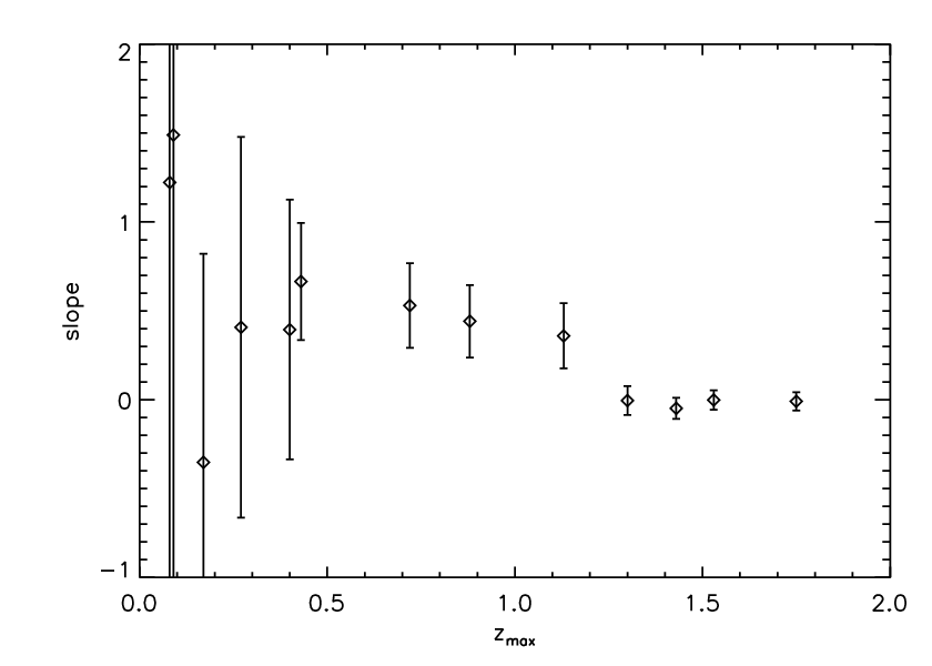
Thus, by fitting a single line from to we see evidence for acceleration at low , but no clear indication of acceleration or deceleration when all redshifts up to are considered. This analysis cannot provide an estimate for the redshift of acceleration onset.
A bilinear fit on the other hand, can give a model-independent estimate of the transition redshift . We perform a continuous piecewise linear fit dividing the data in two redshift intervals: from redshift 0 to and from to . In this way yields an estimate of the acceleration redshift . As before, the reduced chisquares are always : any gives formally an acceptable fit. However, the chisquare changes significantly as a function of the parameters. The top panel of figure 7 shows the best fit (acceleration slope and deceleration slope for the best fit ). The bottom panel shows the chisquare as a function of . Note that while goodness of fit tests considers the absolute value of and all values of pass the goodness of fit test, parameter estimation procedure only considers differences from the minimum. The bottom panel of Fig. 7 clearly shows that when looking at , the data constrain ; in particular, at 1- level. This may indicate that the error-bars may be over-estimated or highly correlated.


The above analysis has been carried out without reference to any specific model of the energy content of the universe, nor to any specific theory of gravity. We have assumed, however, homogeneity and isotropy at large scales, so that the FLRW geometry can be considered a good approximation. In addition, the method used to obtain four out of the fourteen data-points used in this section (those coming from differentiating Supernovae data) assumes spatial flatness.
5 Conclusions
Combining different distance measurements is a powerful tool to constrain cosmological parameters. Comparing them instead helps constrain possible deviations from the assumptions underlying the standard cosmological model or exotic physics. We have considered Supernovae data [17], direct meauserments of cosmic expansion [30, 13] and determinations of the BAO scale [25, 10].
We have explored the possibility of uniform deviations from “cosmic transparency” through its effects on distance duality, by parameterizing possible deviations from the Etherington relation (1). Such deviations from the Etherington relation might arise from any uniform and “gray” source of attenuation, from astrophysical processes such as gray [1] or replenishing dust [27] (used to try to explain Supernovae results without resorting to cosmic acceleration, or relaxing the constraints on cosmic acceleration), to more exotic physics such as photon-axion mixing [7, 8, 2, 5].
Combining direct meauserments of cosmic expansion [30] and SN data [17], and assuming an underlying flat CDM model, we have placed strong constraints on such deviations, in particular improving the existing constraint [21] by nearly an order of magnitude.
While allowing for such deviations from transparency, we have revisited the reported tension [25] between distance measures obtained from SN and BAO within the CDM model. We have found no discrepancy among Supernova data –even allowing for deviations from transparency– , determinations and high-redshift BAO, indicating that the source of the discrepancy may likely be found among systematic effects in the modelling of low redshift BAO data (or be attributed to a - statistical fluctuation), rather than in exotic physics.
Finally, since Supernovae data and data appear to be highly consistent with each other, we have combined them and attempted to draw some model-independent conclusions about the recent accelerated expansion. We determine the transition redshift between deceleration and recent acceleration to be .
To conclude, we remark that the comparison among distance measurements along the lines of the analysis presented here can also be used to place bounds on possible departures from homogeneity and isotropy. There has been significant activity recently in trying to use comparisons among distance measurements as a powerful tool for probing fundamental assumptions behind cosmological models. For example, Clarkson et al [6] suggest to test the Copernican Principle by examining the consistency condition: where and a prime stands for differentiation with respect to redshift . This condition arises by solving for the curvature energy density parameter from the definition of the luminosity distance in a FLRW universe, and then demanding that its derivative vanishes. In general, deviations form the Copernican Principle may appear as inconsistency between distance measures. The condition above relies on the same consistency relation we used here, that is on the consistency relation that exists within the homogeneous and isotropic FLRW models between luminosity or area distance and the Hubble rate, both as a function of redshift. In particular the Clarkson et al condition is not satisfied for radially inhomogeneous models in general.
While our data are too noisy to perform the test in the form stated above (note that involves first and second derivatives of the data), here, in the language of [6], we have effectively looked at radial deviations from the Copernican Principle by testing consistency between different distance measurements ( and ). We have found no indication of inconsistency among the different datasets/distance measures. In general, radial inhomogeneities would lead to anisotropic clustering, so, for example, the BAO feature in the two-point correlation function would not be isotropic [6], yielding inconsistency between the inferred and . A similar effect is expected in a large class of Bianchi models. We expect that future data will impose interesting constraints on these models.
Acknowledgements
AA would like to thank B. Reid, C. Carbone, J. Miralda-Escudé and J. Garriga for useful discussions. AA is supported by the Institute of Space Sciences (IEEC-CSIC). LV is supported by FP7-PEOPLE-2007-4-3 IRG n 202182, RJ is supported by FP7-PEOPLE-2007-4-3 IRG. LV and RJ are supported by MICINN grant AYA2008-03531. We thank the University of Barcelona and in particular the Institute of Cosmos Sciences for hospitality. We also thank the Galileo Galilei Institute for Theoretical Physics for hospitality and INFN for partial support during the completion of this work. We acknowledge the use of the Supernova Cosmology Project (SCP) “Union” Cosmology Tables and of the Legacy Archive for Microwave Background Data Analysis (LAMBDA). Support for LAMBDA is provided by the NASA Office of Space Science.
References
References
- [1] Aguirre, A. N. 1999, ApJL, 512, L19
- [2] Bassett, B. A., & Kunz, M. 2004, ApJ, 607, 661
- [3] Bassett, B. A., & Kunz, M. 2004, PRD, 69, 101305
- [4] Bovy, J., Hogg, D. W., & Moustakas, J. 2008, ApJ, 688, 198
- [5] Burrage, C. 2008, PRD, 77, 043009
- [6] Claskson, C., Bassett, B., & Hui-Ching Lu, T. 2008, Physical Review Letters, 101, 011301
- [7] Csáki, C., Kaloper, N., & Terning, J. 2002, Physics Letters B, 535, 33
- [8] Csáki, C., Kaloper, N., & Terning, J. 2002, Physical Review Letters, 88, 161302
- [9] Daly, R. A., & Djorgovski, S. G. 2003, ApJ, 597, 9
- [10] Eisenstein, D. J., et al. 2005, ApJ, 633, 560
- [11] Etherington, J. M. H. 1933, Phil. Mag., 15, 761
- [12] Ferramacho, L. D., Blanchard, A., & Zolnierowski, Y. 2008, arXiv:0807.4608
- [13] Freedman, W. L., et al. 2001, ApJ, 553, 47
- [14] Jeffreys, H. 1961, Theory of Probability, 3rd ed., Oxford University Press
- [15] Jimenez, R., Verde, L., Treu, T., & Stern, D. 2003, ApJ, 593, 622
- [16] Komatsu E., et al., 2008, arXiv:0803.0547
- [17] Kowalski et al. 2008, ApJ, 686, 749
- [18] Lazkoz, R., Nesseris, S. & Perivolaropoulos, L. 2008, JCAP 0807 012 [arXiv:0712.1232 [astro-ph]].
- [19] Ménard, B., Nestor, D., Turnshek, D., Quider, A., Richards, G., Chelouche, D., & Rao, S. 2008, MNRAS, 385, 1053
- [20] Mirizzi, A., Raffelt, G. G. & Serpico, P. D. 2005, Phys. Rev. D 72 023501 [arXiv:astro-ph/0506078].
- [21] More, S., Bovy, J., & Hogg, D. W. 2008, arXiv:0810.5553
- [22] Mörtsell, E., & Goobar, A. 2003, Journal of Cosmology and Astro-Particle Physics, 9, 9
- [23] Mörtsell, E., & Goobar, A. 2003, Journal of Cosmology and Astro-Particle Physics, 4, 3
- [24] Mörtsell, E., & Clarkson, C. 2009, Journal of Cosmology and Astro-Particle Physics, 1, 44
- [25] Percival, W. J., Cole, S., Eisenstein, D. J., Nichol, R. C., Peacock, J. A., Pope, A. C., & Szalay, A. S. 2007, MNRAS, 381, 1053
- [26] Perivolaropoulos, L. & Shafieloo, A., arXiv:0811.2802 [astro-ph].
- [27] Riess, A. G., et al. 2004, ApJ, 607, 665
- [28] Riess, A. G., et al. 2007, ApJ, 659, 98
- [29] Seo, H.-J., Siegel, E. R., Eisenstein, D. J., & White, M. 2008, ApJ, 686, 13
- [30] Simon J., et al., 2005, PhRvD, 71, 123001
- [31] Wang, Y., & Tegmark, M. 2005, PRD, 71, 103513