DESY 09-150
, , ,
Planck-scale Lorentz violation constrained by Ultra-High-Energy Cosmic Rays
Abstract
We investigate the consequences of higher dimension Lorentz violating, CPT even kinetic operators that couple standard model fields to a non-zero vector field in an Effective Field Theory framework. Comparing the ultra-high energy cosmic ray spectrum reconstructed in the presence of such terms with data from the Pierre Auger observatory allows us to establish two sided bounds on the coefficients of the mass dimension five and six operators for the proton and pion. Our bounds imply that for both protons and pions, the energy scale of Lorentz symmetry breaking must be well above the Planck scale. In particular, the dimension five operators are constrained at the level of . The magnitude of the dimension six proton coefficient is bounded at the level of except in a narrow range where the pion and proton coefficients are both negative and nearly equal. In this small area, the magnitude of the dimension six proton coefficient must only be below . Constraints on the dimension six pion coefficient are found to be much weaker, but still below .
1 Introduction
Over the last decade there has been consistent theoretical interest in possible high energy violations of local Lorentz Invariance (LI) as well as a flourishing of observational tests. The theoretical interest is driven primarily by hints from Quantum Gravity (QG) ideas that local Lorentz invariance may not be an exact symmetry of the vacuum. The possibility of outright Lorentz symmetry violation (LV) or a different realization of the symmetry than in special relativity has arisen in string theory [1, 2, 3], Loop QG [4, 5, 6], non-commutative geometry [7, 8, 9, 10], space-time foam [11], some brane-world backgrounds [12] and condensed matter analogues of “emergent gravity” [13].
Lorentz symmetry breaking is certainly not a necessary feature of QG, but any Planck-scale induced LV effects could provide an observational window into QG phenomena. Moreover, the absence of LV phenomena provides by itself constraints on viable QG theories and more firmly establishes the validity of special relativity. Unfortunately, it is difficult to directly connect a theory of QG at the Planck scale with low energy, testable physics. To see the difficulty from the traditional standpoint, consider gravity as just an effective field theory (EFT) [14] and simply quantize the spin-2 graviton coupled to the standard model. (This approach is in contrast with large extra dimensions which may have a much lower QG scale [15].) In the EFT approach there must be new quantum gravitational effects to preserve unitarity [16], however the scale of the breakdown of the theory occurs when the center of mass energy in a scattering process nears the Planck scale . This is 15 orders of magnitude higher than what we can directly probe at the LHC with its center of mass beam energy of roughly 10 TeV. Therefore directly or indirectly probing QG with a scattering or other experiment seems out of reach, unless one is in a large extra dimensions scenario. Note however that this scattering argument relies on the Lorentz symmetry of the low energy effective field theory (EFT) - the meaningful Lorentz invariant physical quantity that controls the sensitivity to physics at is the center of mass energy. Quantities that are not LI, such as the energy of a single particle, are irrelevant when asking how QG affects our LI observables, in this case the scattering amplitudes.
On the other hand, if we are specifically testing LI, the situation changes. Here, new quantities must be introduced to describe the physically meaningful LV physics. In particular, not only LI quantities such as particle mass or center of mass energy are considered in defining an observable, but also perhaps LV quantities such as the energy of a particle in some frame, a cosmological propagation distance, etc. These quantities can be enormous, offsetting the tiny Planck scale in a physical observable, thereby magnifying very small corrections (see e.g. [17, 18, 19]). These LV quantities provide leverage and have been referred to as “windows on QG”.
Placing these windows in a well defined framework is vital. The standard approach is to construct a Lagrangian containing the standard model operators and all LV operators of interest11 1 There are other approaches to either violate or modify Lorentz invariance, that do not yield a low energy EFT (see [20] and ref.s therein). However, these models do not easily lend themselves to UHECR constraints as the dynamics of particles is less well understood and hence we do not consider them here.. All renormalizable LV operators that can be added to the standard model are known as the (minimal) Standard Model Extension (mSME) [21]. These operators all have mass dimension three or four and can be further classified by their behavior under CPT. The CPT odd dimension five kinetic terms for QED were written down in [22] while the full set of dimension five operators were analyzed in [23]. The dimension five and six CPT even kinetic terms for QED for particles coupled to a non-zero background vector, which we are primarily interested in here, were partially analyzed in [24]. It is notable that SUSY forbids renormalizable operators for matter coupled to non-zero vectors [25] but permits certain nonrenormalizable operators at mass dimension five and six.
Many of the operators in these various EFT parameterizations of LV have been very tightly constrained via direct observations (see [17] for a review). The exceptions are the dimension five and six CPT even operators, where the LV modifications to the free particle equations of motion are suppressed by small ratios such as or , where and are the particle mass and energy, respectively. All operators can be tightly, albeit indirectly, constrained by EFT arguments [26] as higher dimension LV operators induce large renormalizable ones if we assume no other relevant physics enters between the TeV and energies. This is a very powerful argument and should not be arbitrarily discounted. However, since it is generically expected that new physics may come into play above the TeV scale, this assumption may fail, hence the hierarchy of terms can change. Therefore, it would be nice, if possible, to constrain the dimension five and six LV CPT even kinetic terms directly via observation. This is the purpose of the present work.
How might one do this? As mentioned, the LV corrections for these operators are suppressed by or relative to the LI operators. Hence one would need a very high energy particle or very sensitive experiment to minimize this suppression. The highest energy particles presently observed are ultra high energy cosmic rays (UHECRs). The construction and successful operation of the Pierre Auger Observatory (PAO) has brought UHECRs to the interest of a wide community of scientists. Indeed, this instrument will allow, in the near future, to assess several problems of UHECR physics and also to test fundamental physics with unprecedented precision [27, 28, 29]. As we shall show, it also currently provides an extremely accurate test of Lorentz symmetry following the introduction of these unconstrained operators.
In the past, there have been attempts to use UHECRs as a tool to test scenarios of QG. In particular, the consequences of some realizations of Loop QG were considered in [6], while a pure phenomenological and simplified approach was taken by [30, 31, 32]. Recent studies analyze one of the CPT even dimension four operators (that yield a limiting speed difference between protons and pions) in terms of the UHECR spectrum [33, 34]. In this work we study the consequences of LV induced by the inclusion of CPT even dimension five and six terms in the QED Lagrangian on the UHECR spectrum with energies . By comparing the theoretical reconstructed spectrum with the PAO observed spectrum we derive constraints on the pion and proton dimension six LV coefficients.
This paper is structured as follows. In section 2 we outline the LV theoretical framework we adopt and the assumptions we make in this study. In section 3 we describe the present observational and theoretical status of Cosmic Ray physics. Furthermore, we describe in section 4 the effects of LV on the main processes involved in the propagation of UHECRs, while in section 5 we show the UHECR spectra resulting from our MonteCarlo simulations. Section 6 is devoted to the presentation of the constraints we obtain on the considered LV parameters. Finally, we draw our conclusions.
2 Theoretical framework
In order to study the phenomenological consequences of LV induced by QG, the existence of a dynamical framework in which to compute reactions and reaction rates is essential. We assume that the low energy effects of LV induced by QG can be parameterized in terms of a local EFT22 2 In effect we assume that QG effects decouple and that at low energies they are a perturbation to the standard model + general relativity.. Furthermore, we assume that only boost invariance is broken, while rotations are preserved (see [17] for further comments on rotation breaking in this context). Therefore we introduce LV by coupling standard model fields to a non-zero vector.
We focus on the CPT even mass dimension five and six operators involving a vector field (which we assume to describe the preferred reference frame in which the CMB is seen as isotropic), fermions (whose mass we label ) and photons, that are quadratic in matter fields and hence modify the free field equations. The Lagrangian for a particular species of Dirac fermion is then the usual Dirac term plus
| (1) | |||
where is a timelike unit vector describing the preferred frame, and are the usual right and left projection operators, , and is the gauge covariant derivative. The coefficients are dimensionless. The additional photon operator is
| (2) |
For fermions, at the helicity eigenstates are almost chiral, with mixing due to the particle mass and the dimension five operators. Since we will be interested in high energy states, we re-label the coefficients by helicity, i.e. . The resulting high energy dispersion relation for positive and negative helicity particles can easily be seen from (1) to involve only the appropriate or terms. For compactness, we denote the helicity based dispersion by . Therefore at high energies we have the dispersion relation (see also [35])
| (3) |
where and . We have dropped the terms as the operator present in these terms makes the correction to the equations of motion proportional to and hence tiny.
In Lorentz gauge the photon dispersion relation is
| (4) |
Before we continue, we make a simplifying assumption - that parity is a symmetry in our framework. In particular, this implies that our helicity coefficients are equal. There is no underlying motivation from QG as to why parity should be approximately valid if LI is broken, however it is reasonable to assume this for the first attempt at constraints. The parity violating case, which involves helicity decay reactions in addition to the ones considered here, we leave for future work.
The dimension five fermion operators induce two corrections, one proportional to and one corresponding to a change in the limiting speed of the fermion away from . Constraints on a different limiting speed for pions and protons in the context of UHECR have been derived in [33], if . Complementing this constraint, if then the necessary absence of a vacuum Čerenkov (VC) effect for high energy protons [36] (see section 4.2 for a more detailed discussion of the VC effect) limits . In our parameterization with the parity assumption, the coefficients are therefore immediately constrained at the level. Hence we will drop them for the rest of this paper and concentrate on the dimension six terms.
Since parity is conserved, . We define and , and drop the superscript from . Hence, the dispersion relations we assume in this work for protons, pions, and photons respectively, are
| (5) | |||
Although there are indications that these operators may be strongly constrained [27, 28, 24], nothing conclusive has been claimed yet, as high energy particles are needed to probe the effects of these operators. A fairly accurate general estimate of the energy range in which LV corrections in equations (5) are relevant is obtained by comparing the largest mass of the particles entering in the LV reaction with the magnitude of the LV correction in these equations [36]. In our case, assuming , the typical energy at which LV contributions start to be relevant is of order , a fairly reachable energy for UHECR experiments. Note that if one considers neutrinos, then the typical energy (assuming, as a worst case scenario, ) is , well within reach of neutrino telescopes such as ICECUBE or Km3NeT. However, we will neglect them here, as even the confirmed detection of high energy astrophysical neutrinos has not yet been achieved [37]. Hence, at present, only observations in the field of UHECR physics, with energy of order , can provide significant information on such type of LV.
UHECR’s are, in general, assumed to be composite objects, being either protons or nuclei. In our EFT approach, the fermionic operators apply to the quark constituents, there are other LV operators for gluons, and the proton LV is a combination of all the LV for the constituents. This is the approach taken in [38], where a parton model is assumed for protons and the net proton LV is determined by the LV terms for the partons along with the parton fraction at UHECR energies. If we really want to establish constraints on the bare parameters in the action, we would need to do the same type of analysis. Our goal is not so ambitious - we will treat protons, photons, and pions as individual particles with their own independent dispersion relations and constrain the coefficients. This approach is phenomenologically valid since we are using energy-momentum conservation and the initial and final state particles are separated composite fermions with well-defined energy, momenta, and dispersion relations. These composite dispersion relations are therefore what must appear in the energy-momentum conserving -functions in the scattering amplitude.
It is possible, of course, that one could have LV for quarks and none for hadrons if LV was possible only for particles with color charge. In this case our results would be very misleading. However, since we assume that LV comes from QG and not a modification of QCD we do not give this possibility much credence and so will ignore it. Hence, underlying our treatment is the assumption that CPT even dimension six operators for the fundamental partons generate net CPT even dimension six operators for the composite particles of the same order. Results derived by treating every particle as independent in this way are weaker than what one might get using a parton approach, where many different particles are made of only a few constituents.
Now that we have our theoretical background, we turn to the UHECR spectrum.
3 Cosmic Ray spectrum
The Cosmic Ray spectrum spans more than ten decades in energy (from to ) with a power-law shape of impressive regularity
| (6) |
The spectral slope has been measured as for , followed by a softening (the “knee”) to for , a further steepening to (the “second knee”) up to and a subsequent hardening (the “ankle”) to again at [39, 40].
One of the most puzzling problems in CR physics concerns their origin. Being charged particles, their paths are deflected in both Galactic and extragalactic magnetic fields during propagation, erasing the information about their source direction, resulting in their observed arrival directions being almost isotropically distributed. Only CRs with sufficient energy, , are capable of remaining predominantly undeflected by nG extragalactic magnetic fields [41], leading to the expectation of some anisotropy, as was found experimentally [42]. In fact, the expected angle of deflection due to, e.g., galactic magnetic fields (GMFs), is (we assume as the typical coherence length of the GMFs and a mean field strength of ) [42]
| (7) |
decreasing as the proton energy increases due to the reduced fraction of the proton’s energy in the field.
A second CR puzzle regards the “cross-over” energy at which the sources of the cosmic rays detected at Earth change from being predominantly Galactic to extragalactic. Interestingly, lower limit constraints have been placed on this transition energy using the ultra-high energy neutrino flux observation limits set by AMANDA observations [43, 44], with too low a transition energy requiring too large an energy budget for extragalactic sources, resulting in the possibility of the expected ultra-high energy neutrino fluxes being in conflict with the observational limits (under certain assumptions about the source acceleration efficiency, evolution with redshift, and UHECR spectral index). However, the energy of the transition to a dominance of extragalactic cosmic ray sources continues to remain unclear. It is natural to expect a flattening of the energy spectrum at the transition energy, with the harder subdominant extragalactic component taking over from the softer Galactic component. In this respect, associating the “ankle” feature with the cross-over energy certainly provides a coherent picture for the transition. At this energy the (proton) Larmor radius in the Galaxy’s G field begins to exceed the thickness of the Milky Way disk and one expects the Galactic component of the spectrum to die out. Subsequently, the end-point of the Galactic flux ought to be dominated by heavy nuclei, as these have a smaller Larmor radius for a given energy, and some data is indeed consistent with a transition from heavy nuclei to a lighter composition at the ankle [45, 46, 47].
A third puzzle regarding CRs is at what energy the end-point to the CR spectrum occurs. A suppression to the spectrum is naturally expected theoretically due to the interactions of UHECR protons with the Cosmic Microwave Background (CMB). This interaction leads to the production of charged and neutral pions, eventually dumping the energy of the UHECR protons into neutrinos and -rays. At the present epoch, significant photo-pion production in a LI theory occurs only if the energy of the interacting proton is above , with a rapid decrease in their mean-free-path above this energy. Hence, it has long been thought to be responsible for a cut-off in the UHECR spectrum, the Greisen-Zatsepin-Kuzmin (GZK) cut-off [48]. Moreover, trans-GZK particles arriving at Earth must be accelerated within the so called GZK sphere, whose radius is expected to be of the order of 100 Mpc at and to shrink down at larger energies. A simple analytic description of the GZK sphere can be given (see A),
| (8) |
with and . Experimentally, the presence of a suppression of the UHECR spectrum has been confirmed only recently with the observations by the HiRes detector [49] and the PAO [50]. Although the cut-off could be also due to the finite acceleration power of the UHECR sources, the fact that it occurs at roughly the expected energy favors a GZK explanation. The correlation results shown in [42] further strengthen this hypothesis. It is this last puzzle where possible LV effects come into play.
4 UHECR Proton Interactions and LV
As they propagate from their source to Earth, UHECRs lose their energy in several ways. Besides adiabatic losses due to the expansion of the Universe, whose LV modifications will be neglected in the following, the most relevant energy loss mechanisms for protons are pair production through interactions with the CMB (dominant in the present epoch for ) and photo-pion production through interactions with the CMB (dominant in the present epoch for ). The typical loss time-scales for these processes are shown in Fig. 1.

The effect of LV on UHECR propagation is twofold: it modifies standard reactions and allows new, normally forbidden reactions. In particular, in the following subsection we will consider
- •
, which is modified by LV.
- •
and , which correspond respectively to photon and pion emission in vacuum and would be forbidden if LI were exact.
Before moving to a detailed description of these processes in a LV framework, it is worth discussing the role played by the possible presence of nuclei in UHECRs, as supported by increasing experimental evidence [47]. Let us consider here how our proton LV terms also affect UHECR nuclei propagation. At Earth, a given cosmic ray heavy nuclei has a certain total momentum . Assuming the total momentum is equally distributed amongst the constituent nucleons, each nucleon possesses a momentum , where is the mass number of the nucleus. A iron nuclei () at eV then has nucleons with momenta only at eV. This is much lower than the individual protons we are considering at momenta eV, and since our LV scales heavily with momenta the propagation of heavy nuclei is largely unaffected by LV. We assume therefore the interactions of heavy nuclei may be treated as if LI was still exact.
Since nuclei propagation remains unaffected by the LV terms discussed in this paper, the results from previous work on nuclei propagation such as [41, 51, 52] remain applicable here. The general conclusion from this work is that a variety of source compositions, from protons to iron nuclei, can be consistently assumed to be the sole injection composition at each CR source, without being in conflict with either the CR spectrum or elongation rate data.
However, in order to get clear constraints and in agreement with the evidence on the anisotropic distribution for UHECR recently reported by AUGER [42], we shall assume here a purely protonic flux at the energies of our interests.
4.1 Modified GZK
In a LI theory, photo-pion production is the highest energy-loss process that occurs during the propagation of UHECR protons. It is therefore crucial to carefully investigate how LV affects its characteristics. The most important quantities needed to compute the UHECR spectrum are the mean-free-path of protons and the fraction of initial proton momentum transferred to the outgoing pion, the so called inelasticity .
4.1.1 LV mean-free-path
We want to calculate the mean-free-path for a proton undergoing GZK interactions with the CMB. We assume here that LV does not strongly affect the dynamics of the photo-pion production, hence that the LV cross section is roughly equal to the LI one, apart from small corrections that we neglect. We discuss below the potential effects of LV on the cross-section. Assuming the LV dispersion relations outlined in Eq. (5), with , the mean-free-path can be calculated as
| (9) |
where is the energy of the incoming photon, is the number density of the target photons (which are isotropically distributed in space), the photon threshold energy depends in general on , and , is the total cross-section, dependent on the “square center of mass energy” , is the velocity of the proton with energy and is the angle between the direction of the incoming photon and that of the incoming proton.
4.1.2 Comments on phase space effects
In the computation above we neglected direct contributions to the total cross-section coming from LV. The total cross-section is calculated as
| (13) |
where and is the angle between the incoming and the outgoing proton. This quantity is related to the LI Mandelstam variable .
In order to evaluate LV corrections to the total cross-section we have to consider different possible contributions from both kinematics and dynamics. While we do not expect dynamical contributions (i.e. from ) to be relevant, because, by analogy with findings in LV QED [56], they are Planck-suppressed with respect to ordinary ones, corrections to the kinematics could in principle play an important rôle. However, in the LI case the differential cross-section is known to be strongly peaked at , i.e. in the forward direction, with an exponential suppression of high-transverse momentum production [53], which is usually modeled, for small values of , as
| (14) |
where as determined experimentally (notice that by construction33 3 The careful reader might be worried by the fact that this is no longer ensured in LV physics, hence one could have at some energy for some combination of the LV parameters. However, we notice that the condition sets the onset of the process of Čerenkov emission in vacuum (which we discuss in section 4.2). Since for each combination of LV parameters we consider the GZK reaction only at energies below the VC threshold, the condition is guaranteed.).
We expect then that only LV corrections affecting the behavior of near are important for our estimate of the total cross section , being other corrections exponentially suppressed. In order to estimate how is affected by LV physics, we numerically compare the expectation values of in both LI and LV cases for various configurations of the interacting particles. We find that LV contributions are indeed relevant in the region . However, we notice that neglecting LV effects in the cross-section is a conservative approach. In fact, it is possible to show that the way LV affects the cross-section is such that it enhances distortions from the LI GZK process. Indeed, when the threshold energy is lowered (hence, protons are able to interact with more photons) the cross-section is increased (hence, the probability of interaction is enhanced as well), while when the threshold energy is increased the cross-section is lowered. Therefore, neglecting LV effects in the cross-section amounts to underestimating LV effects in UHECR proton propagation, thereby implying conservative limits.
4.1.3 LV inelasticity
The other important quantity entering in the computation of the UHECR spectrum is the proton attenuation length for photo-pion production onto the radiation background. The attenuation length expresses the mean distance over which a proton must travel to reduce its energy to of its initial one and is usually defined as [55]
| (15) |
where
| (16) |
is the inelasticity of the process as computed in the LI case for the single pion emission process. At threshold, , giving, . At energies well above threshold, the multiplicity of the photo-pion production process grows and the above equation for the inelasticity no longer holds.
The computation of is an issue, since we need to compute the energy-momentum conservation also in off-threshold configurations. However, since LV corrections to are relevant only near threshold (in the LV case as increases as well) we assume that Eq. (16) is valid for .
The problem is then reduced to what to assume for around , where the LV corrections are in principle important. As for the total cross-section, we assume that the analytic expression (16) is not modified provided is computed taking into account LV. In order to check our assumption, we notice that we are able to compute easily the expected value of at threshold, because the solution for of the energy-momentum conservation (12), together with the requirement that is minimum, provides us with the pair , or equivalently . We find that, as long as , this procedure is valid, as the values obtained by extrapolating Eq. (16) down to are well in agreement, within , with . If instead , then the numerically evaluated inelasticity may differ significantly from the extrapolated one. However, in this case the inelasticity is dramatically reduced (or dramatically increased, to , when ), compared to the LI one, reaching values of . When this happens, protons do not lose their energy effectively (or they do lose most of it in just one interaction) during propagation, which leads to clear inconsistencies with experimental observations, as will be shown below.
4.2 Vacuum Čerenkov emission
LV allows two more processes competing with the photo-pion-production to be active: photon and pion VC emission. In fact, due to LV a proton can spontaneously emit photons (or neutral pions) without violating energy-momentum conservation.
It has been shown in other contexts (LV QED [36, 56]) that the reaction rate for such processes is of the order of a nanosecond, acting then as a sharp effective cut-off on the particle spectrum. We follow the same analysis as in [56], for pion as well as photon emission, but considering our operators. For the case of pion emission we use the Yukawa nucleon-pion matrix element. A straightforward calculation shows that the VC rates for both photons and pions become extremely fast very quickly above threshold. Hence computing the threshold energies of both processes and cutting off the spectrum at those energies is sufficient for our aims, the typical VC time scales being many orders of magnitude shorter than the time scales of the other processes involved in UHECR propagation. We implement the cut-off by setting the attenuation length for particles above VC threshold to the value .
Let us first discuss VC with emitted photons, as it will be the simpler case. The threshold energy depends, in general, on both and . Our goal, however is to constrain and , not . Hence we need a simplification such that becomes irrelevant, which will allow us to place a constraint only on . We can achieve such a simplification by considering only low energy photon emission. Since the dispersion correction scales as , LV is irrelevant for low energy photons unless is unnaturally large. Hence we can ignore for soft photon emission. The photon VC effect then becomes very similar to the ordinary Čerenkov effect, where there is Čerenkov emission when the group velocity of a particle exceeds the low energy speed of light. This happens at some UHECR momenta provided .
One might be concerned that considering only low energy photon emission, which is a small part of the outgoing phase space, would give a rate that is too low to give our sharp cut-off. This can be shown explicitly to not be the case. For example, if we assume of O(1) and , which is unnaturally large, then we can neglect for photon energies up to one-hundredth the initial proton energy. This provides easily enough phase space to yield a high rate directly above threshold, justifying the cut-off implementation mentioned above. We therefore impose a cut-off to the UHECR spectrum in the half-plane at momentum
| (17) |
On the other hand, we treat pion VC differently. We want to limit both and , hence we will consider both hard and soft pion emission. This means that we use the whole outgoing phase space. However, we lose the ability to analytically solve the threshold equations. Instead, the pion VC threshold energy has to be computed numerically as
| (18) |
where, as usual, is the fraction of initial momentum going to the pion. Note that where this equation has no real solution, pion VC does not occur.
5 Results
5.1 Monte Carlo simulation to obtain GZK feature
During UHE proton propagation, the dominant energy-loss process leading to attenuation at the highest energies occurs via photo-pion production, (note the pion multiplicity is 1 for interactions close to threshold), as shown in Fig. 1. This process has a typical inelasticity of the order of 20% (see Eq. 16), meaning that each time it interacts, a proton loses roughly of its total energy. Moreover, the attenuation length of a UHECR proton is roughly a few Mpc, as highlighted by Eq. (25) and seen in Fig. 5. UHECRs then undergo between 1 and 10 photo-pion production interactions during their journey from source to Earth, but not substantially more. Therefore, it is not justified to think of this energy-loss process as if it was happening continuously. Rather, a MonteCarlo approach should be adopted, to take into account the stochastic nature of the GZK process.
In order to understand the main effects of LV on the UHECR spectrum we present the results of pure proton composition of UHECRs under the assumption of a continuous distribution of sources, distributed as
| (19) | |||||
where describes the number of sources in a comoving volume element and is the redshift at which the source density is being considered. The free parameter is varied to investigate the effects of the closest source, which might be non-trivial. Indeed, if LI were exact, UHECR protons in the cut-off region would only travel distances , hence only local () sources can actually contribute to the arriving flux at these energies. Therefore, LI spectrum reconstruction is mildly affected by the actual value of as we shall see later. However, if LI is violated this conclusion could be changed, as protons may travel substantially longer distances without losing energy. Along with this, the spectrum of CRs injected by each source was assumed to be of the form,
| (20) | |||||
Throughout this paper, and will be used unless stated otherwise. In what follows we investigate both the effect on the arriving CR flux introduced by our LV terms as well as the effect of introducing a mimimum distance to the first source. Such a minimum distance consideration is introduced to enable the reader to differentiate the effect this has on the GZK feature from the effects introduced by the LV terms.
5.2 LV effects on the cut-off feature
By employing a Monte Carlo description for the propagation of UHECR protons, including the effects introduced through the consideration of the LV terms discussed, we obtain the expected fluxes arriving at Earth following the injection of protons with spectra of the form shown in Eq. (20) at their sources, whose spatial distribution is given in Eq. (19), with .
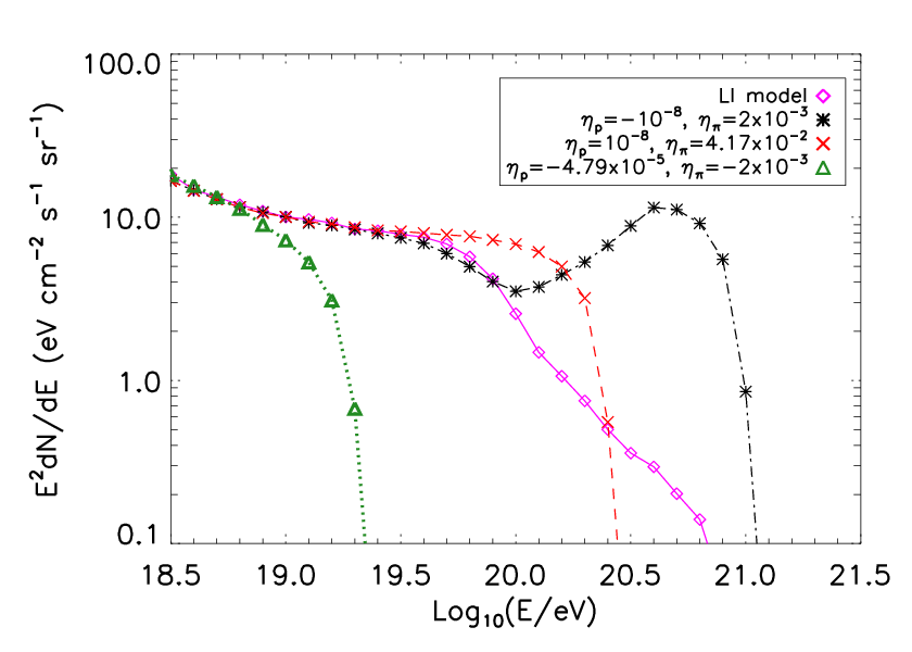
In Fig. 2 we show the almost complete range of results obtainable from Monte Carlo simulations for the propagation of UHECR protons including our LV effects, for different LV parameters and . The LV term effects vary from a simple complete GZK-like cut-off (with or without recovery as in the case of a GZK-suppression) of the proton flux, to a early (or delayed) onset of the cut-off to higher energies followed by a stronger cut-off when it occurs.
We now describe the main features in more detail. Firstly, the effect of VC emission is clearly evident, as seen in the green dotted curve. The VC emission acts as a sharp cut off on the UHECR spectrum. Note that since this cut-off is at the source there is not only the effect of the hard cutoff in the spectrum at , but also a suppression of the UHECR flux at lower energies due to the absence of the higher energy source protons that would have wound up with eV at Earth due to GZK losses.
Secondly, for the case of and , corresponding to the red dashed curve, the GZK cut-off feature is seen to be delayed compared to the LI case, turning on very quickly at around . Interestingly, this is a general effect seen in all cases for “large” (compared to ). In all such cases, the cut-off feature exhibited is both initially () delayed and very hard after turning on. Note that to understand this second effect of delay plus strong cut off considering only the effects of VC emission is not sufficient, since VC depends only on in the first quadrant, whereas we see that changes in affect the UHECR spectrum. The delay is easily understood, though, as positive increases the effective mass of the pion, thereby delaying the GZK cutoff. The cutoff is sharper since, for any given background photon energy, once the reaction occurs the phase space opens up more rapidly than in the LI case due to the scaling of the LV dispersion corrections with energy.
The black solid curve shows another important effect. In this case, , while . While for the chosen combination of parameters the GZK feature turns on at nearly the LI energy (compare the black and the magenta curve), the spectrum exhibits a strong enhancement of the flux above . The reason is that if then the effective pion mass is increased at high energy, hence the GZK process can be effectively inhibited. We have thus that high energy ( in the case of Fig. 2) protons are no longer absorbed by the photon radiation fields. A similar feature of flux recovery has been found also in [33].
5.3 Effects of distance to the closest source on the cut-off feature
In order to distinguish the effects that LV terms may introduce to the GZK cut-off feature, we here consider the effects on this cut-off feature introduced by non-zero values of on a LI spectrum model. In Fig. 3 we show the results for the spectra obtained using different . By increasing the distance between the first UHECR source and Earth, the high energy GZK feature is seen to become much steeper as has been demonstrated previously in [57]. With the effects introduced by the existence of a non-zero in mind, the differences this introduces into the shape of the cut-off feature compared to that introduced by LV terms are demonstrated to be quite distinct, with LV terms typically leading to a harder cut-off in the energy spectrum than usually expected from LI calculations.

6 Constraints from UHECR observations
UHECR observations indeed provide strong constraints on the available LV parameter space.
We consider first of all the fact that protons with energy have been observed. A straightforward constraint is then implied by the fact that these protons do not lose a significant amount of their energy through VC emission during propagation. In order to be able to reproduce the highest energy point of AUGER data (whose energy is about ), we are forced to demand
| (21) |
Photon VC emission does not depend on the pion LV coefficient, but it may happen only if , according to Eq. (17), hence it places a limit only on . On the other hand, for some combinations of pion VC emission may become the dominant energy loss channel for UHECR protons. The portion of parameter space allowed by Eq. 21 is the red region in Fig. 4. However, this constraint is not as robust as it would seem at first sight, as the measured flux at this energy is compatible with 0 at Confidence Level (CL). From this point of view, it is safer to place a VC constraint at a slightly lower energy than the maximum one. We decide then to consider as our reference energy , which corresponds to the highest energy AUGER observation which is not compatible with 0 at . The constraint obtained in this way is shown as the blue region in Fig. 4.

Further tightening of this region might be achieved by considering modifications of the GZK reaction. We will neglect in the following the region , which is strongly constrained by VC, and we run MonteCarlo simulations in the region
We also consider the lines and .
A strategy would seem most suitable in order to check different (,) LV models against experimental data. Data are taken from [50]. It is interesting to notice that there are values of the pair that provide a better fit of data than the LI model. In particular, the minimum of the () occurs for , while the associated to the LI propagation model is of the order of 6.8. However, since we have more parameters available one would expect such a lowering of the value. Only major progress in both theoretical and experimental understanding of the UHECR spectrum could lead to better discrimination between LI and LV best-fit models.
Using the best fit value of the , constraints at 95% and 99% CL can be placed, respectively, at and (see [58] for further details). The green circles and black crosses in Fig. 4 represent points in the parameter space allowed at 95% and 99% CL respectively. We notice that there is no allowed point in the quadrant . In fact, the recovery feature we found in this region of the parameter space is so strong that even the smallest values of the LV parameters we considered produce UHECR spectra incompatible with data.
Summarizing, the final constraints implied by UHECR physics are (at 99% CL)
| (22) | |||||
As it can be noticed, the constraint is placed at one of the edges of our simulation field. This is due to the fact that for protons of energy above lose energy dramatically in pion production, while below this energy they do not effectively interact with the radiation backgrounds. The combination of these two effects yields a GZK-like feature, in statistical agreement with data44 4 It is interesting to note that the situation in which both coefficients are negative and equal is envisaged in other frameworks of LV, such as [2]. However, due to renormalization group flow this equality, even if realized at the QG scale, would not generically hold for UHECR energy scales without an ad hoc symmetry or other mechanism to protect it.. We checked, however, that for more negative values of the LV parameters this effect happens at too low energy to be compatible with data. Hence, this constraint is robust.
7 Conclusions
In this work we have investigated the consequences of relaxing the assumption of Lorentz invariance in the physics of UHECRs. Motivated by naturalness arguments we focused on a particular realisation of LV in which it is described by the addition, in an EFT context, of mass dimension five and six CPT even operators to the Standard Model Lagrangian.
A careful analysis of the physics intervening in the propagation of protons with energy allowed us to identify how LV would modify the arriving spectrum of UHECRs at Earth. Due to photo-hadronic interactions with CMB photons, the spectrum of UHECRs is expected to be suppressed above a certain energy, corresponding to the threshold energy at which the GZK process becomes effective. The strength of the suppression depends upon physical uncertainties about the UHECR sources, such as the distance of the closest source from Earth (because the mean-free-path of protons for such a process is of the order of few Mpc). However, we found that the effect of LV is not degenerate with this uncertainty, and can give rise to a very distinct signature entirely unexpected in the LI case. A detailed observation of the GZK cut-off may therefore, in principle, be used to probe the presence of LV effects at these energies, e.g. through the observation of a recovery of the spectrum at high energies.
Moreover, we are able to generalize and to strengthen the constraints on and compared to previous works. On the one hand we considered the full parameter space, with only one simplifying assumption, parity, on the LV coefficients. On the other hand, we placed robust constraints, through a careful statistical analysis of the agreement between model expectations and observational data, strengthening by more than four orders of magnitude previous limits in some regions of the parameter space.
However, this analysis also shows that significant improvements on constraints of LV obtained using this method will be possible only when better data becomes available. Improvements on both statistics and energy resolution of data at energies are definitely needed to achieve this.
Acknowledgements
LM acknowledges support from SISSA during the early stages of preparation of this work.
Appendix A Simple Analytic Form for UHECR Proton Attenuation
Assuming that the interaction occurs predominantly at the onset of the -resonance (), whose width is assumed to be , we can write the interaction rate given in Eq. (11) as
| (23) |
where is the photon threshold energy in the proton rest frame corresponding to the resonance, is the width of the -resonance, is the photon number energy distribution and mb is the interaction cross section. Assuming that corresponds to the CMB spectrum, at a temperature K, Eq. (23) can be re-written as,
| (24) |
where , , , and eV. Since at threshold eV, at threshold the integral probes the region. With the inelasticity of these collisions being roughly 20%, the corresponding attenuation lengths are
| (25) |
where Mpc, and eV. Equation (25) is represented in Fig. 5, where it is compared to the results of a full numerical computation of the GZK horizon.

References
References
- [1] V. A. Kostelecky and S. Samuel, Phys. Rev. D 39, 683 (1989).
- [2] J. R. Ellis, N. E. Mavromatos and D. V. Nanopoulos, Phys. Lett. B 665, 412 (2008) [arXiv:0804.3566 [hep-th]].
- [3] P. Horava, arXiv:0901.3775 [hep-th].
- [4] R. Gambini and J. Pullin, Phys. Rev. D 59, 124021 (1999).
- [5] C. Rovelli and S. Speziale, Phys. Rev. D 67, 064019 (2003) [arXiv:gr-qc/0205108].
- [6] J. Alfaro and G. Palma, Phys. Rev. D 67 (2003) 083003 [arXiv:hep-th/0208193].
- [7] S. M. Carroll, J. A. Harvey, V. A. Kostelecky, C. D. Lane and T. Okamoto, Phys. Rev. Lett. 87, 141601 (2001).
- [8] J. Lukierski, H. Ruegg and W. J. Zakrzewski, Annals Phys. 243 (1995) 90 [arXiv:hep-th/9312153].
- [9] G. Amelino-Camelia and S. Majid, Int. J. Mod. Phys. A 15 (2000) 4301 [arXiv:hep-th/9907110].
- [10] M. Chaichian, P. P. Kulish, K. Nishijima and A. Tureanu, Phys. Lett. B 604, 98 (2004) [arXiv:hep-th/0408069].
- [11] G. Amelino-Camelia, J. R. Ellis, N. E. Mavromatos, D. V. Nanopoulos and S. Sarkar, Nature 393, 763 (1998).
- [12] C. P. Burgess, J. Cline, E. Filotas, J. Matias and G. D. Moore, JHEP 0203, 043 (2002).
- [13] C. Barcelo, S. Liberati and M. Visser, “Analogue gravity,” Living Rev. Rel. 8, 12 (2005). [arXiv:gr-qc/0505065].
- [14] C. P. Burgess, Living Rev. Rel. 7, 5 (2004) [arXiv:gr-qc/0311082].
- [15] N. Arkani-Hamed, S. Dimopoulos and G. Dvali, Phys. Lett. B 429 (1998) 263; L. Randall and R. Sundrum, Phys. Rev. Lett. 83 (1999) 3370; Phys. Rev. Lett. 83 (1999) 4690.
- [16] T. Han and S. Willenbrock, Phys. Lett. B 616, 215 (2005) [arXiv:hep-ph/0404182].
- [17] D. Mattingly, Living Rev. Rel. 8, 5 (2005)
- [18] G. Amelino-Camelia, New J. Phys. 6 (2004) 188 [arXiv:gr-qc/0212002].
- [19] O. Bertolami, Gen. Rel. Grav. 34 (2002) 707 [arXiv:astro-ph/0012462].
- [20] G. Amelino-Camelia, arXiv:0806.0339 [gr-qc].
- [21] D. Colladay and V. A. Kostelecky, Phys. Rev. D 58, 116002 (1998) [arXiv:hep-ph/9809521].
- [22] R. C. Myers and M. Pospelov, Phys. Rev. Lett. 90 (2003) 211601 [arXiv:hep-ph/0301124].
- [23] P. A. Bolokhov and M. Pospelov, Phys. Rev. D 77, 025022 (2008) [arXiv:hep-ph/0703291].
- [24] D. Mattingly, arXiv:0802.1561 [gr-qc].
- [25] S. Groot Nibbelink and M. Pospelov, Phys. Rev. Lett. 94, 081601 (2005) [arXiv:hep-ph/0404271].
- [26] J. Collins, A. Perez, D. Sudarsky, L. Urrutia and H. Vucetich, Phys. Rev. Lett. 93, 191301 (2004) [arXiv:gr-qc/0403053].
- [27] M. Galaverni and G. Sigl, Phys. Rev. Lett., 100, 021102 (2008). arXiv:0708.1737 [astro-ph].
- [28] L. Maccione and S. Liberati, arXiv:0805.2548 [astro-ph].
- [29] M. Galaverni and G. Sigl, Phys. Rev. D 78 (2008) 063003 [arXiv:0807.1210 [astro-ph]].
- [30] R. Aloisio, P. Blasi, P. L. Ghia and A. F. Grillo, Phys. Rev. D 62 (2000) 053010 [arXiv:astro-ph/0001258].
- [31] F. W. Stecker and S. T. Scully, Astropart. Phys. 23 (2005) 203 [arXiv:astro-ph/0412495].
- [32] L. Gonzalez-Mestres, arXiv:0902.0994 [astro-ph.HE].
- [33] S. T. Scully and F. W. Stecker, arXiv:0811.2230 [astro-ph].
- [34] X. J. Bi, Z. Cao, Y. Li and Q. Yuan, arXiv:0812.0121 [astro-ph].
- [35] L. A. Glinka, arXiv:0812.0551 [hep-th].
- [36] T. Jacobson, S. Liberati and D. Mattingly, Phys. Rev. D 67 (2003) 124011 [arXiv:hep-ph/0209264].
- [37] T. I. Collaboration, arXiv:0809.1646 [astro-ph].
- [38] O. Gagnon and G. D. Moore, Phys. Rev. D 70 (2004) 065002 [arXiv:hep-ph/0404196].
- [39] T. K. Gaisser and T. Stanev, Nucl. Phys. A 777 (2006) 98.
- [40] D. R. Bergman and J. W. Belz, J. Phys. G 34, R359 (2007) [arXiv:0704.3721 [astro-ph]].
- [41] D. Hooper, S. Sarkar and A. M. Taylor, Astropart. Phys. 27 (2007) 199 [arXiv:astro-ph/0608085].
- [42] J. Abraham et al. [Pierre Auger Collaboration], Science 318 (2007) 938 [arXiv:0711.2256 [astro-ph]].
- [43] M. Ahlers, L. A. Anchordoqui, H. Goldberg, F. Halzen, A. Ringwald and T. J. Weiler, Phys. Rev. D 72 (2005) 023001 [arXiv:astro-ph/0503229].
- [44] M. Ahlers, L. A. Anchordoqui and S. Sarkar, arXiv:0902.3993 [astro-ph.HE].
- [45] D. Allard, E. Parizot and A. V. Olinto, Astropart. Phys. 27, 61 (2007) [arXiv:astro-ph/0512345].
- [46] V. Berezinsky, arXiv:0710.2750 [astro-ph].
- [47] M. Unger [The Pierre Auger Collaboration], arXiv:0706.1495 [astro-ph].
- [48] K. Greisen, Phys. Rev. Lett. 16 (1966) 748; Zatsepin, Kuzmin, Sov.Phys.JETP 4, 78.
- [49] R. Abbasi et al. [HiRes Collaboration], arXiv:astro-ph/0703099.
- [50] M. Roth [Pierre Auger Collaboration], arXiv:0706.2096 [astro-ph].
- [51] D. Hooper, S. Sarkar and A. M. Taylor, Phys. Rev. D 77 (2008) 103007 [arXiv:0802.1538 [astro-ph]].
- [52] D. Allard, N. G. Busca, G. Decerprit, A. V. Olinto and E. Parizot, JCAP 0810 (2008) 033 [arXiv:0805.4779 [astro-ph]].
- [53] A. Mucke, R. Engel, J. P. Rachen, R. J. Protheroe and T. Stanev, Comput. Phys. Commun. 124 (2000) 290 [arXiv:astro-ph/9903478].
- [54] D. Mattingly, T. Jacobson and S. Liberati, Phys. Rev. D 67 (2003) 124012 [arXiv:hep-ph/0211466].
- [55] F. W. Stecker, Phys. Rev. Lett. 21 (1968) 1016.
- [56] T. Jacobson, S. Liberati and D. Mattingly, Annals Phys. 321 (2006) 150 [arXiv:astro-ph/0505267].
- [57] V. Berezinsky, A. Z. Gazizov and S. I. Grigorieva, Phys. Rev. D 74 (2006) 043005 [arXiv:hep-ph/0204357].
- [58] W.-M. Yao W M et al. [The Particle Data Group] 2006 J. Phys. G 33 1