Dynamic Transitions in a Two Dimensional Associating Lattice Gas Model
Abstract
Using Monte Carlo simulations we investigate some new aspects of the phase diagram and the behavior of the diffusion coefficient in an associating lattice gas (ALG) model on different regions of the phase diagram. The ALG model combines a two dimensional lattice gas where particles interact through a soft core potential and orientational degrees of freedom. The competition between soft core potential and directional attractive forces results in a high density liquid phase, a low density liquid phase, and a gas phase. Besides anomalies in the behavior of the density with the temperature at constant pressure and of the diffusion coefficient with density at constant temperature are also found. The two liquid phases are separated by a coexistence line that ends in a bicritical point. The low density liquid phase is separated from the gas phase by a coexistence line that ends in tricritical point. The bicritical and tricritical points are linked by a critical -line. The high density liquid phase and the fluid phases are separated by a second critical line. We then investigate how the diffusion coefficient behaves on different regions of the chemical potential-temperature phase diagram. We find that diffusivity undergoes two types of dynamic transitions: a fragile-to-strong transition when the critical -line is crossed by decreasing the temperature at a constant chemical potential; and a strong-to-strong transition when the -critical line is crossed by decreasing the temperature at a constant chemical potential.
pacs
64.70.Pf, 82.70.Dd, 83.10.Rs, 61.20.JaI Introduction
The study of the properties of supercooled water is motivated by its well known anomalous thermodynamic behavior. Besides the density anomaly, the response functions for water appear to diverge at a singular temperature [1]. This apparent divergence of the response functions led to the hypotheses of the existence of liquid polimorphism and of a second critical point, at [2]. In spite of the enormous attention given to this possible singularity, as well as to the many other anomalies, no unique explanation has yet been established. The hypothetical singular point is hidden below the homogeneous nucleation temperature [3] in an experimentally inaccessible temperature range for bulk supercooled water. This rules out direct experimental investigation of this region in order to confirm the existence of liquid-liquid coexistence. In order to circumvent this difficulty, it has been proposed, recently, that a dynamic crossover of the transport properties such as the self-diffusion constant, , and the viscosity, , at temperatures above , would indicate the presence of a critical point [4][5]. The dynamic crossover has also been associated with liquid-liquid transitions in silicon [6] and in non-tetrahedral liquids [7].
The basic surmise behind the link between the dynamic crossover and the presence of a second critical point goes as follows. The liquid-liquid coexistence line that separates two liquid phases terminates at a critical point. Beyond this point, at which the response functions diverge, one finds lines of maxima of these functions which assymptotically approach the critical point. This extension of the first-order phase boundary into the one-phase region is the Widom line at . Even though this line does not exhibit any thermodynamic transition, experiments on water show that the specific heat, shear viscosity and thermal diffusivity [8] exhibit a peak when crossing the Widom line. In particular, Maruyama et. al [9] conducted experiments in nanopores (to avoid homogeneous nucleation) at ambient pressure that present a peak at the constant pressure specific heat at . This temperature coincides (within the experimental error bar) with that one temperature obtained by Xu et. al [10], for the location of the dynamic crossover suggesting that this crossover occurs at the Widom line, confirming the presence of the second critical point.
Unfortunately, the presence of a peak in the specific heat in a certain region of the pressure-temperature phase-diagram is not exclusivity of Widom lines. For instance, in glassformers an abrupt heat capacity drop is observed when ergodicity is broken. This change can happen very sharply in the case of fragile liquids or it may take tens of degrees in the case of strong liquids. Examples of fragile liquids are toluene and metallic systems, while covalent and network forming systems are strong liquids [11]. In the last case, the increase in the specific heat can be simply a smeared peak, located above the melting temperature,, like in the case of and of [12][13][14][15][16] [17]. In the case of strong liquids, it is also possible to observe a weak transition at a temperature between the glass transition temperature, , and the melting temperature, . This peak in the specific heat curve occurs in the tail of a thermodynamic transition where there is a little heat capacity to loose [18]. Example of such strong liquids are the tetrahedral bonded liquids such as water, Si and Ge. This implies that observing a fragile-to-strong crossover in a region where the specific heat grows does not univocally imply the presence of a critical point. An interesting question, however, would be: does the presence of criticality result in a fragile-to-strong crossover?
In order to address this point, in this paper we analyze a model that exhibits two different critical lines and we explore what happens with the dynamics close to these line, in order to test if a fragil-to-strong transition would be a signature for criticality. The present model is an Associating Lattice Gas (Henriques and Barbosa) that corresponds to a lattice gas with hydrogen bonds representede through ice variables. A competition between the filling up of the lattice and the formation of an open four-bonded orientational structure is naturally introduced in terms of the ice bonding variables, and no ad hoc addition of density or bond strength variations is needed. Besides the gas phase and as a result of this competition, the model exhibits two liquid phases that bare resemblance to the two liquid phases predicted for water, corresponding to a low density liquid phase and a high density liquid phase. Moreover, it has both the diffusion and the density anomalies present in water [19].
Here, the model phase diagram is reviewed and analyzed for the presence of dynamic transitions. Two new critical lines were found beyond the liquid-liquid coexsitence line. We searched for fragile to strong transitions in the proximity of these two lines. Comparison between the behaviors of the specific heat and of the diffusion constant in these regions may help in understanding if the type of dynamic transition observed in confined water necessarily means the presence of criticality.
The remaining of this article goes as follows. In sec. II, the lattice model is reviewed, for clarity. In sec. III, results for the chemical potential-temperature phase-diagram are shown and discussed. Our investigation of diffusion is presented in sec. IV. Sec V is a final section of conclusions.
II The Model
We consider a two-dimensional lattice gas model of size on a triangular lattice as introduced by Henriques and Barbosa [20]. In this model, particles are represented by an occupational variable, , which assumes the value , if the site is empty, or , if the site is full, and six orientational variables, , that represent the different orientations that the particle might exhibit. If two neighboring sites have complementary orientations, a hydrogen bond is formed. Four bonding variables are the ice bonding arms: two donors, with , and two acceptors, with . The other two arms, with , do not form bonds, and are taken always opposite to each other, as illustrated in Fig.(1). There is no restriction for donor/acceptor arms positions, thus there are eighteen possible states for each occupied site.
The Hamiltonian includes two contributions: an isotropic, van der Waals like interaction, while the second interaction depends on the orientational degrees of freedom. Two neighboring sites, and , with pointing arms and , form a hydrogen bond if the product between their orientational variables is given by , yielding an energy per site . For a non-bonding pair of occupied sites, the energy per site is , for . In spite of the fact that each molecule may have six neighbors, only four hydrogen bonds per particle are allowed. The overall energy of the system is given by
| (1) |
where are occupation variables, represent the arm state variables, the summation is over neighboring sites.

Comparing the energies of the model at zero temperature two liquid phases, a low density (LDL) and high density (HDL) liquid phase are found, besides the gas phase. Fig.(2) illustrates the HDL and LDL phases. For high values of the chemical potential the lattice is fully occupied ( density ) and the energy per site is . At lower values of the chemical potential, , the soft core repulsion becomes dominant, and the lattice becomes filled, with density and energy per site . Like every other lattice gas, the model exhibits a gas phase, at very low chemical potentials.
At zero temperature, the grand potential per site, , is given by
| (2) |
By equating the grand potential of different phases, we find that the high density phase (HDL) coexists with the low density phase (LDL) at the reduced chemical potential . The coexistence between the LDL and the gas phases occurs at .

The properties of the system at finite temperatures were obtained from Monte Carlo simulations in the grand canonical ensemble, through the Metropolis algorithm. We present a detailed study of the model system, for . Some finite size scaling analysis was also undertaken, when necessary. Interaction parameters were fixed at , which corresponds to ”repulsive” van der Waals interaction. Reduced parameters are defined by
| (3) | |||||
Equilibrium transitions were investigated through analysis of the system specific heat. First-order transitions point were located from hysteresis. The constant volume specific heat was calculated from simulation data obtained at constant chemical potential through the expression
| (5) |
adapted from [21] to the lattice. is the density, is the volume and with .
III The Phase Diagram
The chemical potential-temperature phase diagram of the model was partially analyzed in previous work [20], which focused on the coexistence lines between the low and high density liquids. In this paper the phase-diagram is complemented by the analysis of the region beyond the coexistence line.
The complete phase-diagram is illustrated in Fig.(3) and goes as follows. At low reduced chemical potentials, , for all reduced temperatures, only the gas phase is present. As the reduced chemical potential increases a low density liquid phase appears. This phase coexists with the gas phase along a first-order transition line at . For even higher reduced chemical potentials a high density liquid phase emerges. This phase coexists with the low density liquid phase at the first-order line . But what happens at the end of the two first-order lines?
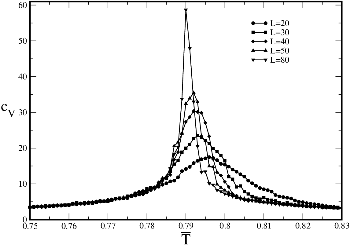
In order to answer the question, we have examined the specific heat at constant volume, , as a function of temperature, for fixed values of , in two regions of the phase diagram: between the two coexistence lines and above the LDL-HDL coexistence line. Fig.(4) illustrates our results. For , between the two coexistence lines, has a peak at a reduced temperature , suggesting the presence of criticality. Similar behavior was observed for every investigated chemical potential between the two coexistence lines, indicating the presence of a critical line. We called this line and represented it in Fig.(3) through a dotted line and square symbols. Above the liquid-liquid coexistence line, for , the specific heat, , displays also a peak at . We have examined a range of chemical potentials above the LDL-HDL coexistence line. A line of maxima of these peaks, named was added to the phase diagram, as shown in in Fig.(3) (dashed line and circles).
In order to check the nature of the two lines, and , in Fig. (3), the specific heat within these regions was computed for different lattice sizes (L=10, 20, 30, 40, 50, 80 and 100). Fig.(5) illustrates the behavior of for for various lattice sizes, showing a diverging peak, as . Fig.(6) shows for , for various lattice sizes. In this case, however, the peak increases mildly with .
The criticality of and was investigated by calculating the energy cumulant given by
| (6) |
Fig.(7) illustrates the energy cumulant for , showing the signature for criticality. Fig.(8) illustrates the energy cumulant for that also indicates the presence of criticality.
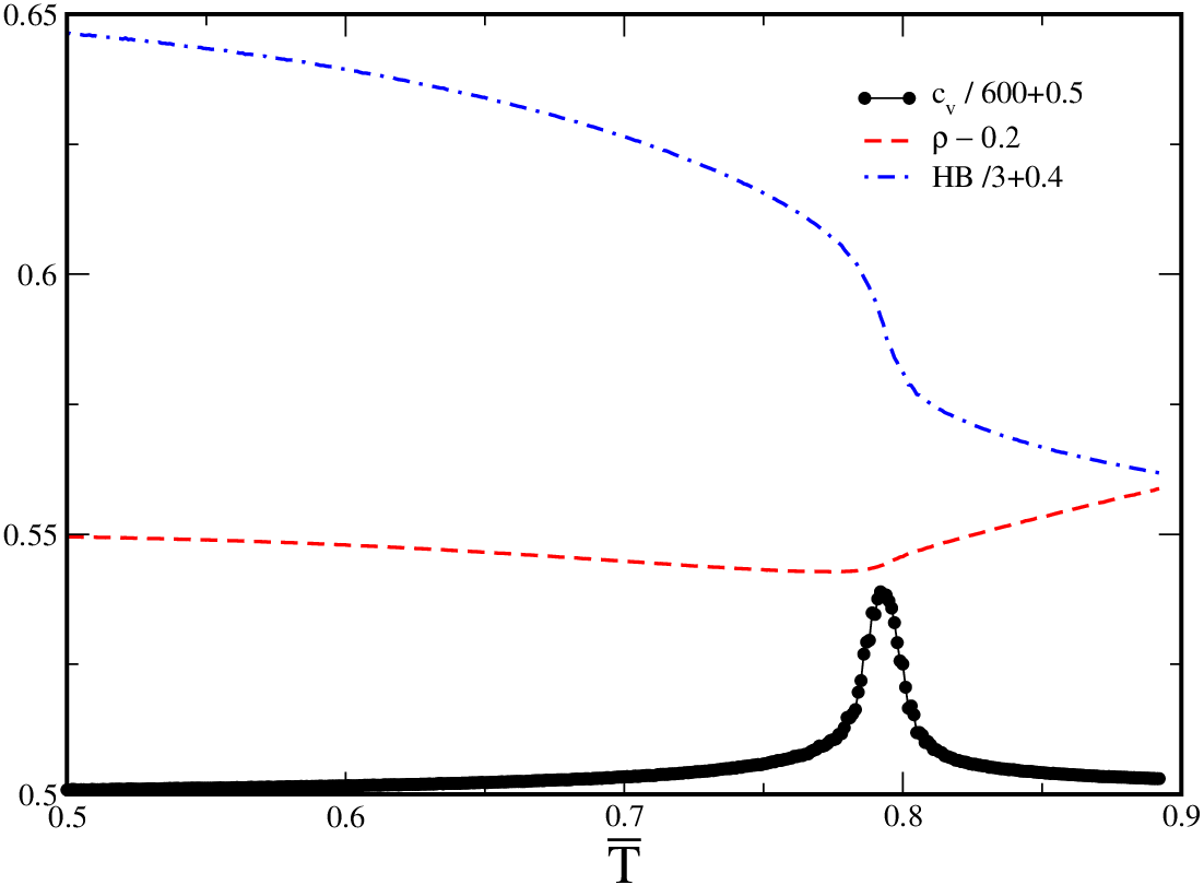
In the attempt to understand the differences between the two transitions, it is important to stablish what is the structural difference between the LDL, HDL, the high and the low densities fluid phases. To answer this question it is necessary to establish a measure of how structured is the liquid. We adopt the number of hydrogen bonds per particle, , and its correlation with particle density as such a measure. Fig.(9) shows that, as temperature is decreased towards the specific heat peak position, hydrogen bond density increases, while particle density decreases. This is indicative that bonding is accompanied by particles abandoning the lattice. On the other hand, in the case of the line, both density and number of bonding particles increase as the temperature decrease towards the peak temperature, as shown in Fig.(10). Thus, in this case, bonding and lattice filling occur simultaneously. Fig.(11) compares the behavior of bond density over the two transitions, while Figs. (12) and (13) illustrate the difference in density behavior. In the case of the transition, as temperature decreases towards the LDL phase, the density, shown in Fig.(12), decreases drastically . At the transition, the system orders itself by forming hydrogen bonds and by releasing nonbonded particles. For temperatures below the transition, the density increases. As for the line, density , shown in Fig.(13),increases smoothly as temperature is lowered.






A closer look of this idea is possible if one examines the behavior of the two densities on different sublattices. Inspection of Fig.(2) suggests dividing the lattice into four sublattices, as illustrated in Fig.(14). Figs.(15) and (18) display sublattice density variations and how the number of hydrogen bonds changes with temperature, in the critical region, for . A clear critical transition is seen, in which one sublattice becomes empty, while the other three get ordered. Figs.(17) and (18) illustrate density variations and the number of hydrogen bonds of the four sublattices with temperature, in the transition region, . In this case, both densities of the four sublattices change smoothly.
Analysis of the sublattice data shows that is an order-disorder transition in which, as the temperature is decreased from the disordered fluid phase, bonds are formed, while nonbonded sites become empty. This critical line joins the two coexistence lines at a tricritical point, , and a bicritical point, .
IV Dynamics
In order to quantify mobility in supercooled liquids, the concept of fragility was introduced by Angell [22]. Analyzing relaxation as a function of temperature, liquids are classified as strong, when relaxation follows an Arrhenius law, or fragile, when the relaxation follows a non-Arrhenius law. Strong liquids present structure that is preserved when temperature is increased, whereas in fragile liquids this structure is easily broken, as temperature increases.
Within the framework of the Adam-Gibbs theory [23], viscous liquids are described as being made of clusters that rearrange cooperatively in order to pass through the free energy barrier. Consequently, diffusion depends on this cooperative rearrangement of the clusters through equation
| (7) |
for the diffusion constant . Here and are constants, is the free energy barrier which the clusters have to overcome. is the configurational entropy, given by
| (8) |
that describes how the structure of the liquid changes with temperature. In Eq.(8) is the Kauzmann temperature [22](for which ) and is the difference in specific heat between the crystal and the liquid configurations, at temperature . If , is temperature independent, the diffusion follows an Arrhenius law, the liquid is very structured and the system is a strong liquid. If the configurational entropy depends on temperature, , Eq.(7) becomes a Vogel-Fulcher equation, the liquid is not structured and is classified as a fragile liquid.
Now we investigate the dynamic properties on crossing the and the lines, at constant chemical potential (see Fig. (3)), by analysing behavior of model diffusivity. In order to compute diffusion coefficient we first equilibrate the system at fixed chemical potential and temperature. In equilibrium this system has particles. Starting from this equilibrium configuration at a time , each one of these particles is allowed to move to an empty neighbor site randomly chosen. The movement is accepted if the total energy of the system is reduced, otherwise it is accepted with a probability where is the difference between the energy of the system after and before the movement. After repeating this procedure times, the mean square displacement per particle at a time is given by
| (9) |
where is the particle position at the initial time and is the particle position at a time . In Eq. (11), the average is taken over all particles and over different initial configurations. The diffusion coefficient is then obtained from Einstein’s relation
| (10) |
Since the time is measured in Monte Carlo time steps and the distance in number of lattice distance, a dimensionless diffusion coefficient is defined as
| (11) |
where and is the distance between two neighbor sites and is the time in Monte Carlo steps.
Figs.(19(a)) - (19(d)) illustrate the behavior of the diffusion constant with the inverse of the reduced temperature , for fixed values of the reduced chemical potentials () At higher temperatures, diffusivity follows a non-Arrhenius trend, namely
| (12) |
indicating that the low density disordered fluid phase is a fragile liquid. At lower temperatures, diffusivity displays Arrhenius behavior, given by
| (13) |
thus characterizing the low density ordered liquid phase as a strong liquid. are fitting parameters in both equations.


This change in dynamics over the critical line occurs because the liquid is structurally different on both sides of the critical line. In the low density disordered fluid phase, interstitial particles weaken the hydrogen bonds and disrupt the network, so particles can rearrange fast and the process of diffusion is not energy activated. In the LDL phase, the network is fully developed, resulting in an ordered liquid, in which particles are ”trapped”, increasing relaxation time and characterizing this phase as a strong liquid, in which an energy activated diffusion process takes place. This is the dynamic transition observed when crossing a Widom line in ramp-like models [10][24], which suggests that the dynamic transition is not linked with the type of line but with the structuring of the system if this happens with or without a thermodynamic phase-transition. The system becomes more organized, as can be seen from the drastic change in the density of the sublattices shown in Fig. (15) with a smooth change in the total density.
Since the HDL is also a structured phase, in principle a fragile-strong transition in the dynamics of diffusion could also be expected on crossing the line. However, this is not the case. Figs.(20(a)) - (20(c)) illustrate the behavior of the diffusion constant as function of inverse temperature, , for fixed chemical potentials and . At higher temperatures and high chemical potentials (or equivalently high densities), the fluid phase has an Arrhenius behavior and so it is a strong liquid. At lower temperatures, the HDL phase also displays an Arrhenius behavior, and therefore is also a strong liquid. The HDL phase and high density fluid phases are both strong liquids that differ in the activation energy. In resume, when the system crosses the line, we have a dynamic transition, and a strong-strong crossover is observed. In this case, the activation energy of the HDL phase is higher than the activation energy of the high density fluid phase, indicating that the HDL phase is more ordered than the high density fluid phase. Diffusion is lowered in the HDL phase because particles spend more time trying to rearrange, in comparison with the high density fluid phase.
How can we explain the existence of a fragile-to-strong crossover on the critical -line and a strong-to-strong transition on the line? The answer is given by the structure of the liquid, described in the previous section. On crossing the -line, the hydrogen-bonded net breaks down abruptly (see Fig. 16), while the -line is accompanied by a much smoother melting of the h-bond network (see Fig.18 ). The difference in the change of structure on crossing one and the other lines is even clearer if one looks at sublattice densities. See Fig.(15) and Fig.(17).
V Conclusions
In this paper we have analyzed equilibrium and dynamic properties of the Associating Lattice Gas Model, a lattice gas with hydrogen bonds represented through ice variables. Competition between the filling up of the lattice and the formation of an open four-bonded orientational structure leads to the presence of two liquid phases and a gas phase. The coexistence lines between the LDL and the gas phases, and between the LDL and HDL phases are connected by a critical -line. Besides the -line, a second one, the -line, also emerges from the LDL-HDL coexistence line. This line is also identified by a peak in the specific heat.
The system undergoes two kinds of dynamic transitions: one fragile-to-strong (crossing the -line) and a strong-to-strong (crossing the -line). Both dynamic transitions are related with structure of the system. In the fragile-to-strong case, the system change its structure drastically when cross -line, from a disordered structure in high temperatures to an ordered one at low temperatures. In the -line region, the change in structure is more subtle, but again the system undergoes a structural change between two ordered phases.
Our results point out in the direction that criticality does not necessarily means fragil-strong transtion. This change is in fact related to the change of structure that in the present case appears in two very different forms.
Acknowledgments
This work was supported by the Brazilian science agencies CNPq, FINEP, Capes and Fapergs.
References
- [1] R. J. Speedy and C. A. Angell, Journal of Chem. Phys. 65, 851 (1976).
- [2] P.H. Poole, F. Sciortino, U. Essmann and H. E. Stanley, Nature (london) 360, 324 (1992).
- [3] D. H. Rasmussen and A. P. MacKenzie, Interactions in the water-polyvinylpyrrolidone system at low temperatures, Plenum Press, New York, 1972.
- [4] L. Liu, S.-H Chen, A. Faraone, S.-W. Yen and C.-Y. Mou, Phys. Rev. Lett. 95, 117802 (2005).
- [5] S.-H. Chen, F. Mallamace, C.-Y Mou, M. Broccio, C. Corsaro, A. Faraone, A. L. Liu, Proceedings of the National Academy of Science of United States of America, 103 , 12974 (2006).
- [6] S. Sastry and C. A. Angell, Nature Mater,2, 739 (2003).
- [7] L. M. Xu, I. Ehrenberg, S. V. Buldyrev and H. E. Stanley, J. Phys.: Condens. Matter, 18, S2239 (2006).
- [8] M. A. Anisimov, J. V. Sengers and J. M. H. Levelt Sengers, Aqueous Systems at Elevated Temperatures and Pressures: Physical Chemistry in water, Steam and Hydrothermal Solutions, Elsevier Ltd, The Netherlands, 2004.
- [9] S. Maruyama, K. Wakabayashi and M. A. Oguni, Aip Conf. Proceedings, 708, 675 (2004).
- [10] L. Xu, P. Kumar, S. V. Buldyrev, S.-H. Chen, P. Poole, F. Sciortino and H. E. Stanley, Proc. Natl. Acad. Sci. U.S.A., 102, 16558 (2005).
- [11] C. A. Angell, Science, 267 , 1924 (1995).
- [12] P. Richet, Y. Bottinga, L. Denielou, J. P. Petitet and C. Tequi, Geochimica et Cosmochimica Acta, 46, 2639 (1982).
- [13] P. Richet and Y. Bottinga, Comptes Rendus de L. Academie des Sciences Serie II, 295, 1121 (1982).
- [14] S. Tamura, T. Yokokawa and K. J. Niwa, J. Chem. Thermodyn., 7, 633 (1975).
- [15] S. Tamura and T. Yokokawa, Bull. Chem. Soc. Japan, 48, 2542 (1975).
- [16] P. Scheidler, W. Kob, A. Latz, J. Horach and K. Binder, J. Chem. Phys. B, 63, 104204 (2005).
- [17] R. B. Sosman, The properties of silica:American Chem. Soc. Monograph, 27, (1927).
- [18] C. A. Angell, Science, 319 (2008).
- [19] M. M. Szortyka and M. C. Barbosa, Physica A, 380, 27 (2007).
- [20] V. B. Henriques and M. C. Barbosa, Phys. Rev. E, 71, 031504, (2005).
- [21] M. P. Allen and D. J. Tildesley, Computer Simulations of Liquids, Claredon Press, Oxford, 1987.
- [22] C. A. Angell, J. Res. Natl. Stand. Technol., 102, 171 (1997).
- [23] G. Adam and J. H. Gibbs, J. Chem. Phys., 43, 139 (1965).
- [24] L. Xu, S. Buldyrev, C. A. Angell and H. E. Stanley, Phys. Rev. E, 74, 031108 (2006).