Fast Evaluation of Interlace Polynomials on Graphs of Bounded Treewidth

Markus Bläser Christian Hoffmann

Abstract

We consider the multivariate interlace polynomial introduced by Courcelle (2008), which generalizes several interlace polynomials defined by Arratia, Bollobás, and Sorkin (2004) and by Aigner and van der Holst (2004). We present an algorithm to evaluate the multivariate interlace polynomial of a graph with $n$ vertices given a tree decomposition of the graph of width $k$ . The best previously known result (Courcelle 2008) employs a general logical framework and leads to an algorithm with running time $f(k)\cdot n$ , where $f(k)$ is doubly exponential in $k$ . Analyzing the $GF(2)$ -rank of adjacency matrices in the context of tree decompositions, we give a faster and more direct algorithm. Our algorithm uses $2^{3k^{2}+O(k)}\cdot n$ arithmetic operations and can be efficiently implemented in parallel.

1 Introduction

Inspired by some counting problem arising from DNA sequencing [ABCS00], Arratia, Bollobás, and Sorkin defined a graph polynomial which they called interlace polynomial [ABS04a]. It turned out that the interlace polynomial is related [ABS04a, Theorem 24] to the Martin polynomial, which counts the number of edge partitions of a graph into circuits. This polynomial has been defined in Martin’s thesis from 1977 [Mar77] and generalized by Las Vergnas [LV83]. Further work on the Martin polynomial has been pursued [LV81, LV88, Jae88, EM98, EM99, Bol02], including a generalization to isotropic systems [Bou87, Bou88, Bou91, BBD97]. In particular, the Tutte polynomial of a planar graph and the Martin polynomial of its medial graph are related. This implies a connection between the Tutte polynomial and the interlace polynomial (see Ellis-Monaghan and Sarmiento [EMS07] for an explanation).

One way to define the interlace polynomial is by a recursion that uses a graph operation. Arratia et al. used a pivot operation for edges [ABS04a]. This operation is a composition of local complementations to neighbor vertices (see Aigner and van der Holst [AvdH04], where the operations are called switch operations). The orbits of graphs under local complementation are related to error-correcting codes and quantum states, and so is the interlace polynomial as well [DP08].

The interlace polynomial can also be defined by a closed expression using the $GF(2)$ -rank of adjacency matrices [AvdH04, Bou05, EMS06]. This linear algebra approach has been used in several generalizations of the interlace polynomial. In this paper, we consider the multivariate interlace polynomial $C(G)$ defined by Courcelle [Cou08] (see Definition 2.1 below) as it subsumes the two-variable interlace polynomial of Arratia, Bollobás, and Sorkin [ABS04b] and the weighted versions of Traldi [Tra10], as well as the interlace polynomials defined by Aigner and van der Holst [AvdH04]. Furthermore, the interlace polynomials $Q(x,y)$ and $Q_{n}^{HN}$ , which have emerged from a spectral view on the interlace polynomials [RP06], are also special cases of Courcelle’s multivariate interlace polynomial.

1.1 Results and Related Work

Our aim is to present an algorithm that, given a graph $G=(V,E)$ and an evaluation point, i.e. a tuple of numbers $((x_{a})_{a\in V},(y_{a})_{a\in V},u,v)$ , evaluates the multivariate interlace polynomial $C(G)$ at $((x_{a})_{a\in V},(y_{a})_{a\in V},u,v)$ . Whereas this is a $\mathsf{\#P}$ -hard problem in general [BH08], it is fixed parameter tractable with cliquewidth as parameter [Cou08, Theorem 23, Corollary 33]. This is a consequence of the fact that the interlace polynomial is monadic second order logic definable ( $MS_{1}$ definable as defined by Courcelle, Makowsky, and Rotics [CMR01]; see also Courcelle [Cou08, Section 5]).¹¹ 1 Note the following crucial difference with respect to monadic second order logic definability: $MS_{1}$ definable evaluation problems are fixed parameter tractable with cliquewidth as parameter [CMR01, Theorem 31]. $MS_{1}$ is a logic that allows one-sorted structures, the universe of which consists of the vertices of the graph. Set variables range over vertex subsets. On the contrary, $MS_{2}$ is a logic that allows two-sorted structures, the universe of which consists of the vertices and edges of the graph. Set variables range over vertex subsets or edge subsets, which, for instance, enables the definition of the Tutte polynomial in $MS_{2}$ . $MS_{2}$ definable evaluation problems are known to be fixed parameter tractable with treewidth as parameter [CMR01, Theorem 32]. We can not expect that this generalizes to cliquewidth, see Fomin, Golovach, Lokshtanov, and Saurabh [FGLS10]. Such graph polynomials can be evaluated in time $f(k)\cdot n$ , where $n$ is the number of vertices of the graph and $k$ is the cliquewidth. The function $f(k)$ can be very large and is not explicitly stated in most cases. In general, it grows as fast as a tower of exponentials the height of which is proportional to the number of quantifier alternations in the formula describing the graph polynomial [Cou08, Page 34]. In the case of the interlace polynomial, this formula involves two quantifier alternations [Cou08, Lemma 24], [CiO07]. If a graph has tree width $k$ , its cliquewidth is bounded by $2^{k+1}$ [CO00]. Thus, the machinery of monadic second order logic implies the existence of an algorithm that evaluates the interlace polynomial of an $n$ -vertex graph in time $f(k)\cdot n$ , where $k$ is the tree width of the graph and $f(k)$ is at least doubly exponential in $k$ . (In particular, the interlace polynomial of graphs of treewidth 1, that is, of trees, can be evaluated in polynomial time, which also has been observed by Traldi [Tra10].)

The monadic second order logic approach is very general and can be applied not only to the interlace polynomial but to a much wider class of graph polynomials [CMR01]. However, it does not consider characteristic properties of the actual graph polynomial. In this paper, we restrict ourselves to the interlace polynomial so as to exploit its specific properties and to gain a more efficient algorithm (Algorithm 2). Our algorithm performs $2^{3k^{2}+O(k)}n$ arithmetic operations to evaluate Courcelle’s multivariate interlace polynomial (and thus any other version of the interlace polynomial mentioned above) on an $n$ -vertex graph given a tree decomposition of width $k$ (Theorem 6.4). The algorithm can be implemented in parallel using depth polylogarithmic in $n$ (Section 7.2). Apart from evaluating the interlace polynomial, our approach can also be used to compute coefficients of the interlace polynomial, for example so called $d$ -truncations [Cou08, Section 5] (Section 7.3). Our approach is not via logic but via the $GF(2)$ -rank of adjacency matrices, which is specific to the interlace polynomial.

1.2 Obstacles

It has been noticed that the Tutte polynomial and the interlace polynomial are similar in some respect [ABS04b]: Both can be defined by a recursion using a graph operation, both can be defined as closed sums over edge/vertex subsets involving some kind of rank. These similarities suggest that evaluating the interlace polynomial using tree decompositions might work completely analogously to the respective approaches for the Tutte polynomial [And98, Nob98]. This is not the case because of the following problems.

Andrzejak’s algorithm [And98] to evaluate the Tutte polynomial uses the deletion-contraction recursion for the Tutte polynomial (via Negami’s splitting formula [Neg87]). Deletion and contraction of an edge has the nice property that it is compliant with tree decompositions: If we are given the tree decomposition of a graph and we delete (or contract) an edge, the original tree decomposition (or, in the case of edge contraction, a simple modification of it) is a tree decomposition of the modified graph. For the interlace polynomial, on the other hand, the respective graph operation is not compliant with tree decompositions: If we perform the pivot operation from Arratia et al. [ABS04a] on a graph, it is not clear how to obtain a tree decomposition of the modified graph. In particular, a single pivot operation can turn a tree (treewidth 1) into a cycle (treewidth 2), see Fig. 1.

Refer to caption — Figure 1: Edge pivoting, a central graph operation for the interlace polynomial, increases treewidth.

Another problem is that in the Tutte case the recursion formula naturally generalizes from the simplest versions (chromatic polynomial) to the most general ones (it is the defining recursion of the Bollobás-Riordan graph invariant [BR99]; cf. also the recurrence relation of the polynomial of Averbouch, Godlin and Makowsky, which generalizes the Tutte polynomial and the matching polynomial [AGM08]). The interlace polynomial, in contrast, needs more and more complicated recursions when generalizing the vertex-nullity interlace polynomial to the multivariate interlace polynomial²² 2 But note that Traldi reduced a three-term recursion to a two-term recursion [Tra10, Corollary 2.4]. (see Courcelle [Cou08, Proposition 12]).

When we consider Noble’s algorithm [Nob98] and concentrate on the definition of the Tutte / interlace polynomial by sums involving ranks, another problem emerges. In the Tutte case, the rank is an easy to understand graph theoretic value, namely the number of vertices minus the number of connected components. Noble observes that, if a graph is extended by a set of vertices and some edges between the old and the new vertices, the set of all partitions of the new vertices captures all possible types of “behavior” of the rank (i.e. number of connected components) when the new vertices and some or all of the new edges are added. – For the interlace polynomial on the other hand, the rank used in the definition is the rank over $GF(2)$ of the adjacency matrix. Even though there exists a graph theoretic interpretation of this rank [Tra09], it is substantially more involved. Furthermore, an appropriate tool to capture the “rank behavior” when extending a graph (such as vertex partitions in the case of the Tutte polynomial) seems to be missing. The main contribution of this work is to devise such a tool and to prove that it works well with tree decompositions.

1.3 Outline

We compute the interlace polynomial by dynamic programming on the tree decomposition of a graph. To this end, we analyze the behavior of the $GF(2)$ -rank of the adjacency matrix of a graph when the graph is extended by a fixed number of vertices and edges between these new vertices and the existing ones.

Section 2 contains the definition of Courcelle’s multivariate interlace polynomial, which we will consider in this work. We will also fix our notation for tree decompositions there. In Section 3 we present our approach in detail. This includes the motivation and definition of two central terms: extended graphs and scenarios. A scenario captures the behavior of the rank of an adjacency matrix when adding vertices. To define this precisely, we introduce symmetric Gaussian elimination in Section 4. In Section 5, we collect properties of scenarios which enable us to use scenarios with tree decompositions. In Section 6, we describe and analyze our algorithm, which evaluates the interlace polynomial by splitting it into parts according to scenarios. In Section 7 we discuss how our algorithm can be parallelized and used to compute (some of the) coefficients of the interlace polynomial. Finally, in Section 8, we mention directions for further research.

2 Preliminaries

We consider undirected graphs without multiple edges but with self loops allowed. Let $G=(V,E)$ be such a graph and $A\subseteq V$ . By $G[A]$ we denote the subgraph of $G$ induced by $A$ , i.e. $(A,\{e\ |\ e\in E,e\subseteq A\})$ . $G\nabla A$ denotes the graph $G$ with self loops in $A$ toggled, i.e. the graph obtained from $G$ by performing the following operation for each vertex $a\in A$ : if $a$ has a self loop, remove it; if $a$ does not have a self loop, add one.

The adjacency matrix of $G$ is a symmetric square matrix with entries from $\{0,1\}$ . As the matrices that we will consider are adjacency matrices of graphs, we use vertices as column/row indices. Thus, the adjacency matrix of $G$ is a $V\times V$ matrix $M=(m_{uv})$ over $\{0,1\}$ with $m_{uv}=1$ iff $uv\in E$ . Furthermore, we will refer to entries and submatrices by specifying first the rows and then the columns: the $(u,v)$ -entry of $M=(m_{uv})$ is $m_{uv}$ , the $A\times B$ submatrix of $M$ is the submatrix of the entries of $M$ with row index in $A$ and column index in $B$ . All matrix ranks will be ranks over the field with two elements, $\{0,1\}=GF(2)$ , i.e. $+$ is XOR and $\cdot$ is AND. Slightly abusing notation we write $\operatorname{rk}(G)$ for the rank of the adjacency matrix of the graph $G$ . The nullity (or co-rank) of an $n\times n$ matrix $M$ is $\operatorname{n}(M)=n-\operatorname{rk}(M)$ . If $G$ is a graph, we write $\operatorname{n}(G)$ for the nullity of the adjacency matrix of $G$ .

Graph polynomials are, from a formal perspective, mappings of graphs to polynomials that respect graph isomorphism. We will consider a multivariate graph polynomial, the multivariate interlace polynomial. To define such a polynomial, one has to distinguish “ordinary” indeterminates from $G$ -indexed indeterminates. For instance, $x$ being a $G$ -indexed indeterminate means that for each vertex $a$ of $G$ there is a different indeterminate $x_{a}$ . If $A\subseteq V$ , we write $x_{A}$ for $\prod_{a\in A}x_{a}$ .

Definition 2.1 (Courcelle [Cou08]).

Let $G=(V,E)$ be an undirected graph. The multivariate interlace polynomial is defined as

C(G)=\sum_{\begin{subarray}{c}A,B\subseteq V\\ A\cap B=\emptyset\end{subarray}}x_{A}y_{B}u^{\operatorname{rk}((G\nabla B)[A\cup B])}v^{\operatorname{n}((G\nabla B)[A\cup B])},

(1)

where $u,v$ are called ordinary indeterminates and $x,y$ $G$ -indexed indeterminates.

2.1 Tree Decompositions

We borrow most of our notation from Bodlaender and Koster [BK08]. A tree decomposition of a graph $G=(V,E)$ is a pair $(\{X_{i}\ |\ i\in I\},T=(I,F))$ where $T$ is a tree and each node $i\in I$ has a subset of vertices $X_{i}\subseteq V$ associated to it, called the bag of $i$ , such that the following holds:

1.

Each vertex belongs to at least one bag, that is $\bigcup_{i\in I}X_{i}=V$ .
2.

Each edge is represented by at least one bag, i.e. for all $e=vw\in E$ there is an $i\in I$ with $v,w\in X_{i}$ .
3.

For all vertices $v\in V$ , the set of nodes $\{i\in I\ |\ v\in X_{i}\}$ induces a connected subgraph of $T$ .

The width of a tree decomposition $(\{X_{i}\},T)$ is $\max\{|X_{i}|\ |\ i\in I\}-1$ . The treewidth of a graph $G$ , $\operatorname{tw}(G)$ , is the minimum width over all tree decompositions of $G$ .

Computing the treewidth of a graph is $\mathsf{NP}$ -complete. But given a graph with $n$ vertices, we can compute a tree decomposition of width $k$ (or detect that none exists) using Bodlaender’s algorithm in time $2^{O(k^{3})}n$ [Bod96] (cf. also Downey and Fellows [DF99, Section 6.3]).

To evaluate the interlace polynomial we will use nice tree decompositions. Note that our definition slightly deviates from the usual one³³ 3 Usually, there is no special restriction on the bag size of the root node, and the leaf nodes contain exactly one vertex.. This has no substantial influence on the running time of the algorithms discussed in this work, but it simplifies the presentation. In a nice tree decomposition $(\{X_{i}\},T)$ , $T$ is a rooted tree with $|X_{r}|=0$ for the root $r$ of $T$ , and each node $i$ of $T$ is of one of the following types:

•

Leaf: node $i$ is a leaf of $T$ and $|X_{i}|=0$ .
•

Join: node $i$ has exactly two children $j_{1}$ and $j_{2}$ , and $X_{i}=X_{j_{1}}=X_{j_{2}}$ .
•

Introduce: node $i$ has exactly one child $j$ , and there is a vertex $a\in V\setminus X_{j}$ with $X_{i}=X_{j}\cup\{a\}$ .
•

Forget: node $i$ has exactly one child $j$ , and there is a vertex $a\in V\setminus X_{i}$ with $X_{j}=X_{i}\cup\{a\}$ .

A tree decomposition of width $k$ with $n$ nodes can be converted into a nice tree decomposition of width $k$ with $O(n)$ nodes in time $O(n)\cdot\mathsf{poly}(k)$ [Klo94, Lemma 13.1.2, 13.1.3].

For a graph $G$ with a nice tree decomposition $(\{X_{i}\},T)$ , we define

V_{i}=\Bigl(\bigcup\{X_{j}\ |\ \text{$j$ is in the subtree of $T$ with root $i$}\}\Bigr)\setminus X_{i}\quad\text{and}\quad G_{i}=G[V_{i}].

We can think of $G_{i}$ as the subgraph of $G$ induced by all vertices that have already been forgotten below node $i$ .

3 Idea

We will now sketch our idea how to evaluate the interlace polynomial. Our approach is dynamic programming similar to the work of Noble [Nob98]. Let $G$ be a graph for which we want to evaluate the interlace polynomial and $(\{X_{i}\},T)$ a nice tree decomposition of $G$ . For each node $i$ of the tree decomposition, we have defined the graph $G_{i}$ that consists of all vertices in the bags below $i$ that are not in $X_{i}$ . We will compute “parts” of the interlace polynomial of $G_{i}$ . These parts are essentially defined by the answer to the following question: How does the rank of the adjacency matrix of some subgraph of $G_{i}$ increase when we add (some or all) vertices of $X_{i}$ ? For the leaves these parts are trivial. Our algorithm traverses the tree decomposition bottom-up. We will show how to compute the parts of an introduce, forget, or join node from the parts of its child node (children nodes, resp.). At the root node, there is only one part left. This part is the interlace polynomial of $G$ .

Before we go into details, let us remark that the answer to the above question (“How does the rank of the adjacency matrix increase when adding some vertices?”) depends on the internal structure of the graph being extended. Consider the graph on the left hand side in Figure 2. If we extend it by the black vertices, the rank increases by $2$ . But if we use the graph on the left hand side in Figure 3, the same extension causes a rank increase by $4$ .

Let us see how we handle this issue. We start with the following definition.

Definition 3.1 (Extended graph).

Let $G=(V,E)$ be some graph, $V^{\prime},U\subseteq V$ , $V^{\prime}\cap U=\emptyset$ . Then we define ${G}[{{V^{\prime}}},{{U}}]$ to denote $G[V^{\prime}\cup U]$ and call ${G}[{{V^{\prime}}},{{U}}]$ an extended graph, the graph obtained by extending $G[V^{\prime}]$ by $U$ according to $G$ . We call $U$ the extension of ${G}[{{V^{\prime}}},{{U}}]$ .

Let us fix an extension $U$ . We consider all $V^{\prime}\subseteq V(G)$ such that $G[V^{\prime}]$ may be extended by $U$ according to the input graph $G$ . For any such extended graph we ask: “How does the rank of $G[V^{\prime}]$ increase when adding some vertices of $U$ ?”. Our key observation is that the answer to this question can be given without inspecting the actual $G$ if we are provided with a compact description (of size independent of $n=|V(G)|$ ), which we call the scenario of ${G}[{{V^{\prime}}},{{U}}]$ .

The scenario of ${G}[{{V^{\prime}}},{{U}}]$ (Definition 4.4) will be constructed in the following way. Consider $M$ , the adjacency matrix of $G[V^{\prime}\cup U]$ . Perform symmetric Gaussian elimination on $M$ using only the vertices in $V^{\prime}$ (for the details see Section 4). The resulting matrix $M^{\prime}$ is symmetric again and has the same rank as $M$ . Furthermore, $M^{\prime}$ is of a form as in Figure 4: The $V^{\prime}\times V^{\prime}$ submatrix is a symmetric permutation matrix with some additional zero columns/rows. The nonzero entries correspond to edges or self loops (not of the original graph $G$ but of some modified graph that is obtained from $G$ in a well-defined way) “ruling” over their respective columns/rows: The edge between $v_{1}$ and $v_{8}$ rules over columns and rows $v_{1}$ and $v_{8}$ . Here, “to rule” means that the only $1$ s in these columns and rows are the $1$ s at $(v_{1},v_{8})$ and $(v_{8},v_{1})$ . Similarly, the self loop at vertex $v_{5}$ rules over column and row $v_{5}$ . The columns and rows that are ruled by some edge or self loop in $V^{\prime}$ are also empty (i.e. entirely zero) in the $U\times V^{\prime}$ submatrix of $M^{\prime}$ . Some columns/rows are not ruled by any edge or self loop in $V^{\prime}$ , for instance column/row $v_{4}$ . This is because there is neither a self loop at vertex $v_{4}$ nor does it have a neighbor in $V^{\prime}$ . However, $v_{4}$ may have neighbors in $U$ . Thus, column $v_{4}$ of the $U\times V^{\prime}$ submatrix may be any value from $\{0,1\}^{U}$ , which is indicated by the question marks. Also, the contents of the $U\times U$ submatrix is not known to us.

Let us choose a basis of the subspace spanned by the nonzero columns of the $U\times V^{\prime}$ submatrix and call it ${s}^{{U}\times{V^{\prime}}}$ . Let ${s}^{{U}\times{U}}$ be contents of the $U\times U$ submatrix. By this construction, we are able to describe the rank of $M^{\prime}$ as the rank of its $V^{\prime}\times V^{\prime}$ submatrix plus a value that can be computed solely from ${s}^{{U}\times{V^{\prime}}}$ and ${s}^{{U}\times{U}}$ .

This will solve our problem that the rank increase depends on the internal structure of the graph $G[V^{\prime}]$ being extended: all we need to know is the scenario $s=({s}^{{U}\times{V^{\prime}}},{s}^{{U}\times{U}})$ of ${G}[{{V^{\prime}}},{{U}}]$ . From $s$ , without considering $G[V^{\prime}]$ , we can compute in time $\mathsf{poly}(|U|)$ how the rank of the adjacency matrix of $G[V^{\prime}]$ increases when we add some vertices from $U$ . This motivates the following definition.

Definition 3.2 (Scenario).

Let $U$ be an extension, i.e. a finite set of vertices. A scenario of $U$ is a tuple $s=({s}^{{U}\times{V^{\prime}}},{s}^{{U}\times{U}})$ where ${s}^{{U}\times{V^{\prime}}}$ is an ordered set of linearly independent vectors spanning a subspace of $\{0,1\}^{U}$ and ${s}^{{U}\times{U}}$ is a symmetric $(U\times U)$ -matrix with entries from $\{0,1\}$ . A scenario for $k$ vertices is a scenario of some vertex set $U$ with $|U|=k$ .

Let us come back to the evaluation of the interlace polynomial of $G$ using a tree decomposition. Recall that at a node $i$ of the tree decomposition we want to compute “parts” of the interlace polynomial of $G[V_{i}]$ . Essentially every scenario $s$ of $X_{i}$ will define such a part: The interlace polynomial itself is a sum over all induced subgraphs with self loops toggled for some vertices. The part of the interlace polynomial corresponding to scenario $s$ will be the respective sum not over all these graphs but only over the ones such that $s$ is the scenario of ${G}[{{V_{i}}},{{X_{i}}}]$ . This will lead us to (2) in Section 6. To compute the parts of a join, forget and introduce node from the parts of its children nodes (child node, resp.), we will employ Lemma 6.1, 6.2 and 6.3. These are based on the fact that scenarios are compliant with tree decompositions, which we will prove in Section 5 (Lemma 5.1, Lemma 5.3 and Lemma 5.5). An example for the overall procedure of the algorithm is depicted in Figure 5.

The time bound of our algorithm stems from the following observation: The number of parts managed at a node $i$ of the tree decomposition is essentially bounded by the number of scenarios of its bag $X_{i}$ . This number is independent of the size of $G$ and single exponential in the bag size (and thus single exponential in the treewidth of $G$ ):

Lemma 3.3.

Let $U$ be an extension, i.e. a finite set of vertices, $|U|=k$ . There are less than $2^{(3k+1)k/2}$ scenarios of $U$ .

Proof.

The number of symmetric $\{0,1\}$ -matrices of dimension $k\times k$ is $2^{(k+1)k/2}$ , as a symmetric matrix is determined by its left lower half. Thus, there are $2^{(k+1)k/2}$ possibilities for ${s}^{{U}\times{U}}$ .

For ${s}^{{U}\times{V^{\prime}}}$ , there less than $2^{k^{2}}$ possibilities: As there are $2^{k}-1$ non-zero elements of $\{0,1\}^{k}$ , the number of linearly independent subsets of $\{0,1\}^{U}$ with $d$ elements is bounded by $\binom{2^{k}-1}{d}$ . Thus, the number of all linearly independent subsets of $\{0,1\}^{U}$ is at most

\sum_{0\leq d\leq k}\binom{2^{k}-1}{d}\leq(k+1)\binom{2^{k}-1}{k}<2^{k^{2}}.\quad\quad\quad

4 Symmetric Gaussian Elimination

We want to convert adjacency matrices into matrices of a form as in Figure 4 without touching the rank. In order to achieve this, we introduce a special way of performing Gaussian elimination that differs from standard Gaussian elimination in the following way. First, it is symmetric, as in general every column operation is followed by a corresponding row operation. In this way, we maintain the correspondence between rows/columns of the matrix we are manipulating and vertices of a graph. Second, we adhere to a particular order when deciding which entry to use for the next pivot operation. This order is (partially) fixed by the tree decomposition. It is crucial for our proofs of the statements in Sect. 5 that the elimination process proceeds according to this order. Third, we perform symmetric Gaussian elimination using only vertices in a subset $V^{\prime}$ of the vertices: When seeking a pivot entry in a particular row/column, we do not consider all entries of the row/column but only the ones that correspond to edges between vertices in $V^{\prime}$ .

4.1 Elimination with a Single Vertex

Assume we are given a graph $G=(V,E)$ , its adjacency matrix $M$ and a vertex $v$ . We would like to compute the rank of $M$ as the “effect of $v$ on the rank” plus the rank of a submatrix in which we have deleted $v$ . This might not immediately be possible using $M$ itself, but we can achieve it by an appropriate modification of $M$ . Arratia et al. observe that edge pivot and local complementation are such appropriate modifications [ABS04b, Lemma 2, Lemma 5]. For our purposes, we want to control the order of the operations on the adjacency matrix. Thus, we do not use edge pivot and local complementation directly, but define a symmetric Gaussian elimination step on $M$ using $v$ in the following way:

•

If $v$ is an isolated vertex without a self loop, we have situation (1) of Figure 6. Vertex $v$ has no influence on the rank of the adjacency matrix and we can delete the column and row corresponding to $v$ without changing the rank of the adjacency matrix. The result of the elimination step is just $M$ .
•

If $v$ has a self loop, there is a $1$ in the $(v,v)$ -entry of $M$ . The elimination step consists of the following operations. Except for entry $(v,v)$ , we remove all $1$ s in the $v$ -column and $v$ -row using the following pair of operations for each neighbor $u$ of $v$ : First, add the $v$ -column to the $u$ -column. Then, in the modified matrix, add the $v$ -row to the $u$ -row. We denote the result of the whole process by $M\rtimes v$ , which is depicted as (2) in Figure 6. Note that $M\rtimes v$ is symmetric again. The rank of $M$ equals $1$ plus the rank of $M\rtimes v$ with $v$ -column and $v$ -row deleted.

Note that – up to order of the operations – this is local complementation on $v$ : Writing ${G}^{{v}}$ for the local complement of a graph $G$ on vertex $v$ [ABS04b, Definition 4], the adjacency matrix of ${G}^{{v}}$ is $M\rtimes v$ [ABS04b, Proof of Lemma 5].
•

If $v$ is neither isolated nor has a self loop, there is a neighbor $u$ of $v$ . Assume that $u$ does not have a self loop. The $(u,v)$ - and $(v,u)$ -entries of $M$ equal $1$ . The elimination step consists of the following operations. In the first stage, except for $(u,v)$ and $(v,u)$ , we remove all $1$ s in the $v$ -column and $v$ -row. This is accomplished by the following pair of operations for each neighbor $u^{\prime}$ of $v$ , $u^{\prime}\neq u$ : First, add the $u$ -column to the $u^{\prime}$ -column. Then, in the modified matrix, add the $u$ -row to the $u^{\prime}$ -row. Again, performing such a pair of column/row operations keeps a symmetric matrix symmetric. At the end of the first stage the $v$ -column and $v$ -row consist entirely of $0$ s, except for the entry at the $u$ -position, which is $1$ . The second stage proceeds as follows: we add the $v$ -column to every column which has a $1$ in the $u$ -row, and we also add the $v$ -row to every row which has a $1$ in the $u$ -column. At the end of this stage also the $u$ -column and $u$ -row consist only of $0$ s except at the $v$ -position. The result of the second stage is a symmetric matrix again, which we denote by $M\rtimes vu$ . It is depicted as (3) in Figure 6. We do not swap columns/rows, as we must keep the vertices in a particular order, which is determined by the tree decomposition, cf. Section 4.2. The rank of $M$ equals $2$ plus the rank of $M\rtimes vu$ with $u$ - and $v$ -column and $u$ - and $v$ -row deleted. Note that this matrix is also the adjacency matrix of ${G}^{{vu}}[V\setminus\{v,u\}]$ , where ${G}^{{vu}}$ denotes edge pivot of $G$ on vertices $v$ and $u$ [ABS04b, Definition 1, Lemma 2].

If $u$ has a self loop we proceed analogously to obtain a matrix with a structure as (4) in Figure 6. Then we can eliminate the self loop at $u$ by, say, adding column $v$ to column $u$ . (As at this point column $v$ is zero everywhere except at $u$ , only entry $(u,u)$ of the matrix is changed by this operation and the symmetry is not destroyed.) Thus, we obtain a matrix exactly as (3) in Fig. 6.

We can describe the effect of a symmetric elimination step on the entries of the matrix (aside from the entries being set to $0$ ) in the following way.

Lemma 4.1.

Let $M=(m_{ij})$ be an adjacency matrix, let $a$ be a vertex with a self loop, and $m_{yx}$ some entry of $M$ which is not in column or row $a$ , i.e. $a\not\in\{x,y\}$ . Then, after symmetric Gaussian elimination using $a$ , the $(y,x)$ -entry of $M$ will be

(M\rtimes a)_{yx}=m_{yx}+m_{ax}m_{ya}.

Lemma 4.2.

Let $M=(m_{ij})$ be an adjacency matrix, let $a$ be a vertex without a self loop, $ab$ an edge and $m_{yx}$ some entry of $M$ which is not in column or row $a$ or $b$ , i.e. $\{x,y\}\cap\{a,b\}=\emptyset$ . Then, after symmetric Gaussian elimination using $ab$ , the $(y,x)$ -entry of $M$ will be

(M\rtimes ab)_{yx}=m_{yx}+m_{ax}m_{yb}+m_{ya}m_{bx}+m_{ax}m_{ya}m_{bb}.

We prove the statement about edge elimination, the case of self loop elimination is completely analogously.

of Lemma 4.2.

Let us assume that $x\leq y$ (the case $x>y$ is analogous). The situation is depicted in Figure 7. Depending on the $(a,x)$ -entry being $1$ or not, column $b$ is added to column $x$ , which adds the $(y,b)$ -entry to the $(y,x)$ -entry. This gives the term $m_{ax}m_{yb}$ . After that, depending on the $(y,a)$ -entry, row $b$ is added to row $y$ . This adds the actual value of the $(b,x)$ -entry to the $(y,x)$ -entry. By the previous column addition, the actual $(b,x)$ -entry is $m_{bx}+m_{ax}m_{bb}$ . Thus, the row addition contributes a term $m_{ya}(m_{bx}+m_{ax}m_{bb})$ . The second stage has no effect on the $(y,x)$ entry: Column $a$ may be added to some other columns. But at this point of time, column $a$ is entirely zero, except at the $b$ entry. Thus, addition of the $a$ column has no effect on the $(y,x)$ entry. The same is true for addition of the $a$ row. ∎

4.2 Vertex Order, Elimination with Vertex Sets, and the Scenario of an Extended Graph

We want to define symmetric Gaussian elimination using a whole set $V^{\prime}\subseteq V$ of vertices. This means that we perform elimination steps using each vertex from $V^{\prime}$ . The result of this process depends on the order in which we use the vertices for elimination steps. Therefore we introduce an order on the vertices of the graph, which will be computed before the computation of the interlace polynomial starts. We will use this order throughout the rest of the paper. Whenever there could be any ambiguity, we proceed according to this order.

The vertex order we are using must be compliant with the tree decomposition we are using: Whenever a vertex is forgotten, it must be greater than all the vertices which have been forgotten before. Or, equivalently, the vertices in the extension $X_{i}$ must be greater than the vertices in $V_{i}$ for each node $i$ of the tree decomposition. Such an order can be obtained by Algorithm 1.

Algorithm 1 Supplying a vertex order.

1: procedure SupplyVertexOrder

c\leftarrow 1

3: for all nodes

i

, in the order of bottom-up traversal, i.e. each father node is visited after all its children do

4: if

i

is a forget node then

a\leftarrow

vertex being forgotten at node

i

6: give vertex

a

number

c

in the vertex order

c\leftarrow c+1

8: end if

9: end for

10: end procedure

Now we are ready to define elimination using a set of vertices.

Definition 4.3.

Let $V^{\prime}\subseteq V$ be a set of vertices of a graph $G=(V,E)$ with adjacency matrix $M$ . Symmetric Gaussian elimination on $G$ using $V^{\prime}$ is defined as the following process: If $V^{\prime}=\emptyset$ , we are done and $M$ is the output of the symmetric Gaussian elimination process using $V^{\prime}$ . Otherwise, we let $v$ be the minimum vertex in $V^{\prime}$ . If $v$ has a self loop we let $M^{\prime}=M\rtimes v$ . Otherwise, we check whether $v$ has a neighbor $u$ in $V^{\prime}$ . If yes, we let $M^{\prime}=M\rtimes vu$ , where $u$ is the minimum neighbor of $v$ . If no, we let $M^{\prime}=M$ . This concludes the processing of $v$ . To complete the elimination using $V^{\prime}$ , we continue recursively with $V^{\prime}\setminus\{v\}$ in the role of $V^{\prime}$ and $M^{\prime}$ in the role of $M$ .

We also order vertex vectors (i.e. elements from $\{0,1\}^{U}$ , $U$ some vertex set) and sets of vertex vectors according to the vertex order (lexicographically). This induced order is used for choosing a “minimal” basis in the following definition.

Definition 4.4 (Scenario of an extended graph).

Let ${G}[{{V^{\prime}}},{{U}}]$ be an extended graph obtained by extending $G[V^{\prime}]$ by $U$ according to graph $G=(V,E)$ . Let the vertex order be such that $v^{\prime}<u$ for all $v^{\prime}\in V^{\prime}$ and $u\in U$ . Then the scenario $\operatorname{scen}({G}[{{V^{\prime}}},{{U}}])$ of ${G}[{{V^{\prime}}},{{U}}]$ is defined as follows: Let $M$ be the adjacency matrix of $G[V^{\prime}\cup U]$ . Perform symmetric Gaussian elimination on $M$ using $V^{\prime}$ to obtain $M^{\prime}$ . Let $M^{\prime}_{UV^{\prime}}$ be the $U\times V^{\prime}$ submatrix of $M^{\prime}$ . Consider the column space $W$ of $M^{\prime}_{UV^{\prime}}$ . We can choose a basis of $W$ from the column vectors of $M^{\prime}_{UV^{\prime}}$ . Let ${s}^{{U}\times{V^{\prime}}}$ be the minimal such basis. Let ${s}^{{U}\times{U}}$ be the contents of the $U\times U$ submatrix of $M^{\prime}$ . We define $\operatorname{scen}({G}[{{V^{\prime}}},{{U}}])$ to be $({s}^{{U}\times{V^{\prime}}},{s}^{{U}\times{U}})$ .

The minimal basis ${s}^{{U}\times{V^{\prime}}}$ in the preceding definition can by obtained by the following steps: Start with an empty set of columns and then as often as possible take the minimum column of $M^{\prime}_{UV^{\prime}}$ which is not in the span of the so far collected columns.

5 Scenarios and Nice Tree Decompositions

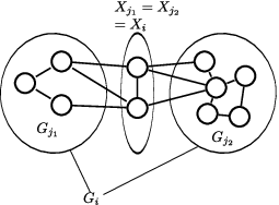
Consider a join node $i$ with children $j_{1}$ and $j_{2}$ in a nice tree decomposition of a graph $G$ the interlace polynomial of which we want to evaluate. By the properties of tree decompositions, this implies a situation as depicted in Figure 8: $G_{j_{1}}=G[V_{j_{1}}]$ and $G_{j_{2}}=G[V_{j_{2}}]$ are disjoint graphs with a common extension $X_{j_{1}}=X_{j_{2}}=X_{i}$ . $G_{i}=G[V_{i}]=G[V_{j_{1}}\cup V_{j_{2}}]$ is the disjoint union of $G_{j_{1}}$ and $G_{j_{2}}$ . Assume that we have computed all parts (see Section 3 and (2)) of the interlace polynomial of $G_{j_{1}}$ and all parts of the interlace polynomial of $G_{j_{2}}$ . From this we want to compute the parts of the interlace polynomial of $G_{i}$ . Consider one such part, say the one corresponding to some scenario $s$ of $X_{i}$ . Somehow we have to find out for which subgraphs⁴⁴ 4 In fact induced subgraphs with self loops toggled at some vertices — but we will ignore this detail for the rest of the section as it is not important to understand the idea. $G[V^{\prime}]$ of $G_{i}$ the scenario of the extended graph ${G}[{{V^{\prime}}},{{X_{i}}}]$ is $s$ . Fortunately, these are exactly the subgraphs $G[V_{1}\cup V_{2}]$ , $V_{1}\subseteq V_{j_{1}}$ , $V_{2}\subseteq V_{j_{2}}$ , with the property that the “join” of the scenario of ${G}[{{V_{1}}},{{X_{j_{1}}}}]$ and the scenario of ${G}[{{V_{2}}},{{X_{j_{2}}}}]$ is $s$ . This is guaranteed by the following lemma.

Lemma 5.1 (Join).

Let $G=(V,E)$ be a graph, $U\subseteq V$ , and $s_{1},s_{2}$ two scenarios of $U$ . Then there is a unique scenario $s_{3}$ of $U$ such that the following holds: If $G[V_{1}]$ and $G[V_{2}]$ are disjoint subgraphs of $G$ that may be extended by $U$ according to $G$ , $\operatorname{scen}({G}[{{V_{1}}},{{U}}])=s_{1}$ , and $\operatorname{scen}({G}[{{V_{2}}},{{U}}])=s_{2}$ , then $\operatorname{scen}({G}[{{V_{1}\cup V_{2}}},{{U}}])=s_{3}$ . Moreover, $s_{3}$ can be computed from $s_{1},s_{2}$ and $G[U]$ within $\mathsf{poly}(|U|)$ steps.

Proof.

We will apply Definition 4.4 to determine $s_{3}$ . We will see that $s_{3}$ is uniquely defined by $s_{1}$ , $s_{2}$ and $G[U]$ , and can be computed from these within the claimed time bound. This will prove the lemma.

Let $G_{1}=G[V_{1}]$ and $G_{2}=G[V_{2}]$ . Let $M$ be the adjacency matrix of $G[V_{1}\cup V_{2}\cup U]$ . As $G_{1}$ and $G_{2}$ are disjoint, $M$ has a form as depicted on the left hand side in Figure 9, the $V_{1}\times V_{2}$ submatrix as well as the $V_{2}\times V_{1}$ submatrix of $M$ consists only of $0$ s.

By Definition 4.4, symmetric Gaussian elimination using $V_{1}\cup V_{2}$ has to be performed on $M$ to obtain $M^{\prime}$ , which is of the form depicted on the right hand side in Figure 9 and from which $s_{3}$ can be read off. Let us analyze a single elimination step occurring during the elimination process in detail, say eliminating with a self loop at a vertex $v\in V_{1}$ . One action in this step is that the $1$ in the $(v,v)$ entry will be used to eliminate another $1$ in the $v$ -row by adding the $v$ -column to the respective column $u$ . Let us argue that this affects neither the $V_{1}\times V_{2}$ submatrix of $M$ nor the $V_{2}\times V_{1}$ submatrix of $M$ . As $v\in V_{1}$ , in the $v$ -row the $V_{2}$ -entries are already $0$ . Thus we know that $u\not\in V_{2}$ , i.e. the $v$ -column will be added to a column from $V_{1}\cup U$ . Thus, the $V_{1}\times V_{2}$ submatrix is not changed. Again as $v\in V_{1}$ , the $V_{2}$ -entries in the $v$ -column are $0$ and addition of the $v$ -column to any other column $u$ does not change the $V_{2}$ -entries of column $u$ . Thus, the $V_{2}\times V_{1}$ submatrix of $M$ is not changed.

Analogous observations can be made for the role of columns and rows reversed (i.e. when adding the $v$ -row to other rows to eliminate $1$ s in the $v$ -column), as well as for elimination steps using an edge between different vertices (instead of self loops). We conclude that symmetric Gaussian elimination steps with $V_{1}$ -vertices affect only the $(V_{1}\cup U)\times(V_{1}\cup U)$ submatrix of $M$ , but not the $V_{1}\times V_{2}$ or $V_{2}\times V_{1}$ submatrix. Analogously, elimination steps with $V_{2}$ -vertices affect only the $(U\cup V_{2})\times(U\cup V_{2})$ submatrix of $M$ . Thus, except for the $U\times U$ submatrix, when performing symmetric Gaussian elimination on $M$ using $V_{1}\cup V_{2}$ , the same things happen as when performing symmetric Gaussian elimination first on $G[V_{1}\cup U]$ using $V_{1}$ and then on $G[V_{2}\cup U]$ using $V_{2}$ . The only difference may be that depending on the vertex order elimination steps with $V_{1}$ -vertices are interlaced with steps using $V_{2}$ vertices. But we argued that $V_{1}$ -elimination steps do not influence parts of $M$ which are relevant for $V_{2}$ -elimination steps and vice versa, so this is not an issue.

As elimination on $M$ using $V_{1}\cup V_{2}$ (yielding $M^{\prime}$ ) on the one hand does the same as elimination on $G[V_{1}\cup U]$ using $V_{1}$ (yielding, say, $M^{(1)}$ ) and elimination on $G[V_{2}\cup U]$ using $V_{2}$ (yielding, say, $M^{(2)}$ ) on the other hand, the $U\times(V_{1}\cup V_{2})$ submatrix of $M^{\prime}$ is just the union of $M^{(1)}_{UV_{1}}$ , the $U\times V_{1}$ submatrix of $M_{1}$ , and $M^{(2)}_{UV_{2}}$ , the $U\times V_{2}$ submatrix of $M_{2}$ . Recall that ${s_{1}}^{{U}\times{V_{1}}}$ and ${s_{2}}^{{U}\times{V_{2}}}$ are minimum bases of the column space of $M^{(1)}_{UV_{1}}$ , $M^{(2)}_{UV_{2}}$ , resp, taken from the columns of these matrices. To compute ${s_{3}}^{{U}\times{(V_{1}\cup V_{2})}}$ , the minimum basis of the column space of the $U\times(V_{1}\cup V_{2})$ submatrix of $M^{\prime}$ taken from the columns of this matrix, we proceed in the following way: Start with the empty set and as long as possible add the minimum vector of ${s_{1}}^{{U}\times{V_{1}}}\cup{s_{2}}^{{U}\times{V_{2}}}$ which is not in the span of the so far collected vectors. This can be done in time polynomial in $|U|$ using standard Gaussian elimination.

The $U\times U$ submatrix is the only part of $M$ which is affected by both, eliminations with $V_{1}$ -vertices and eliminations with $V_{2}$ -vertices. However, the use of the $U\times U$ submatrix is “write-only” during the elimination process: Consider symmetric Gaussian elimination in general, say on some extended graph $G[V^{\prime}\cup U]$ using $V^{\prime}$ . Recall that by Definition 4.3 all the elimination steps will involve only vertices from $V^{\prime}$ in the sense that the step is either $M\rtimes v$ or $M\rtimes vu$ with $u,v\in V^{\prime}$ . Thus, the contents of the $U\times U$ submatrix has no influence on what elimination steps will be performed. All that happens with this submatrix is that column/row vectors are added to it.

Thus, the effect on the $U\times U$ submatrix of all the elimination steps during symmetric Gaussian elimination of $G[V_{1}\cup U]$ using $V_{1}$ can be described as adding a matrix, say $A_{1}$ to the adjacency matrix of $G[U]$ . We can compute $A_{1}$ as $A_{1}={s_{1}}^{{U}\times{U}}-M(G[U])$ , where $M(G[U])$ denotes the adjacency matrix of $G[U]$ . Analogously, we can compute $A_{2}$ which describes the effect of symmetric Gaussian elimination of $G[V_{2}\cup U]$ using $V_{2}$ on the $U\times U$ submatrix. Because of the “write-only” property, the effect of symmetric Gaussian elimination of $M$ using $V_{1}\cup V_{2}$ on the $U\times U$ submatrix of $M$ can be described by $A_{1}+A_{2}$ . Thus we have ${s_{3}}^{{U}\times{U}}=M(G[U])+A_{1}+A_{2}$ , which is the second component of $s_{3}$ . ∎

Definition 5.2.

In the situation of Lemma 5.1 we write $s_{\operatorname{join}}({s_{1}},{s_{2}},{G[U]})$ for $s_{3}$ .

To handle join nodes of the tree decomposition we proved Lemma 5.1: from the scenario of two extended graphs ${G}[{{V_{1}}},{{U}}]$ and ${G}[{{V_{2}}},{{U}}]$ with a common extension $U$ we can compute the scenario of the joined extended graph ${G}[{{V_{1}\cup V_{2}}},{{U}}]$ (cf. Figure 10). To handle also introduce and forget nodes we prove two more lemmas (cf. Figure 11, Figure 12).

Lemma 5.3 (Introduce vertex).

Let $G=(V,E)$ be a graph, $U\subseteq V$ , $s$ a scenario of $U$ , $u\in V\setminus U$ . Then there is a unique scenario $\tilde{s}$ of $\widetilde{U}=U\cup\{u\}$ such that the following holds: If $G[V^{\prime}]$ may be extended by $\widetilde{U}$ according to $G$ , $u$ is not connected to $V^{\prime}$ in $G$ , and $\operatorname{scen}({G}[{{V^{\prime}}},{{U}}])=s$ , then $\operatorname{scen}({G}[{{V^{\prime}}},{{\widetilde{U}}}])=\tilde{s}$ . Moreover, $\tilde{s}$ can be computed from $s$ and $G[\widetilde{U}]$ in $\mathsf{poly}(|U|)$ steps.

Proof.

As $u$ is not connected to $V^{\prime}$ , ${\tilde{s}}^{{\widetilde{U}}\times{V^{\prime}}}$ is ${s}^{{U}\times{V^{\prime}}}$ with a zero component for $u$ added to all the basis vectors. Also, ${\tilde{s}}^{{\widetilde{U}}\times{\widetilde{U}}}$ is just ${s}^{{U}\times{U}}$ with a row and column added representing the neighbors of $u$ in $\widetilde{U}$ . ∎

Definition 5.4.

In the situation of Lemma 5.3 we write $s_{\operatorname{introduce}}({s},{u},{G[\widetilde{U}]})$ for $\tilde{s}$ .

Except for isolated vertices without self loops, every vertex has an effect on the rank of the adjacency matrix [ABS04b, Lemma 2, Lemma 5] (cf. Section 4.1). The following lemma states that this effect can be extracted from the scenario.

Lemma 5.5 (Forget vertex).

Let $G=(V,E)$ be a graph, $u\in U\subseteq V$ , $\widetilde{U}=U\setminus\{u\}$ , $\widetilde{V}=V^{\prime}\cup\{u\}$ , and $s$ a scenario of $U$ . Then there is a unique scenario $\tilde{s}$ of $\widetilde{U}$ and $r\in\{0,1,2\}$ , $n\in\{1,0,-1\}$ such that the following holds: If $G[V^{\prime}]$ is a subgraph of $G$ that may be extended by $U$ according to $G$ , $u>v^{\prime}$ for all $v^{\prime}\in V^{\prime}$ , and $\operatorname{scen}({G}[{{V^{\prime}}},{{U}}])=s$ , then $\operatorname{scen}({G}[{{\widetilde{V}}},{{\widetilde{U}}}])=\tilde{s}$ and the rank (nullity) of the adjacency matrix of $G[\widetilde{V}]$ equals the rank (nullity, resp.) of the adjacency matrix of $G[V^{\prime}]$ plus $r$ ( $n$ , resp.). Moreover, $\tilde{s}$ and $r$ can be computed from $s$ and $G[U]$ in $\mathsf{poly}(|U|)$ steps, and we have $n=1-r$ .

Proof.

Consider the situation after symmetric Gaussian elimination on $G[V^{\prime}\cup U]=G[\widetilde{V}\cup\widetilde{U}]$ using $V^{\prime}$ (Figure 13). We distinguish three cases: (1) there is a basis vector of the $(U\times V^{\prime})$ column space with a $1$ in the $u$ -component, (2) there is no such basis vector, but the $(u,u)$ -entry of the $U\times U$ submatrix equals 1, (3) neither case (1) nor (2).

Let us first consider cases (2) and (3). As all $u$ -components of the vectors in ${s}^{{U}\times{V^{\prime}}}$ are zero, we know that symmetric Gaussian elimination on $G[\widetilde{V}\cup\widetilde{U}]$ using $\widetilde{V}$ will consist of the following two stages: first, exactly the same operations will be performed as in symmetric Gaussian elimination on $G[V^{\prime}\cup U]$ using $V^{\prime}$ (which will end up in the situations depicted in Figure 13 (2), (3)), and then elimination using vertex $u$ will be performed if possible.

Thus, in case (3), $\tilde{s}$ can be obtained from $s$ in the following way: remove the $u$ component of each vector of ${s}^{{U}\times{V^{\prime}}}$ to gain ${\bar{s}}^{{\widetilde{U}}\times{\widetilde{V}}}$ . Let $a$ be the first column of ${s}^{{U}\times{U}}$ . Remove the first component of $a$ . With standard Gaussian elimination, check in time $\mathsf{poly}(|U|)$ if $a$ is in the span of ${\bar{s}}^{{\widetilde{U}}\times{\widetilde{V}}}$ . If it is, let ${\tilde{s}}^{{\widetilde{U}}\times{\widetilde{V}}}={\bar{s}}^{{\widetilde{U}}\times{\widetilde{V}}}$ , otherwise let ${\tilde{s}}^{{\widetilde{U}}\times{\widetilde{V}}}={\bar{s}}^{{\widetilde{U}}\times{\widetilde{V}}}\cup\{a\}$ . Let ${\tilde{s}}^{{\widetilde{U}}\times{\widetilde{U}}}$ be ${s}^{{U}\times{U}}$ with first column and first row deleted. We have $r=0$ and $n=1$ .

In case (2), we first perform an elimination step with the 1 at the $(u,u)$ -entry: let ${\bar{s}}^{{U}\times{U}}={s}^{{U}\times{U}}\rtimes u$ . Then we continue as in case (3) but with ${\bar{s}}^{{U}\times{U}}$ in the role of ${s}^{{U}\times{U}}$ . We have $r=1$ and $n=0$ .

The rest of this proof deals with case (1). Let $w\in V^{\prime}$ be the vertex corresponding to the minimum vector of ${s}^{{U}\times{V^{\prime}}}$ with a $1$ in the $u$ -component (cf. Figure 13 (1)). Compare symmetric Gaussian elimination on $G[V^{\prime}\cup U]$ using $V^{\prime}$ (which is performed to obtain $s$ ) to symmetric Gaussian elimination on $G[\widetilde{V}\cup\widetilde{U}]$ using $\widetilde{V}$ (which is performed to obtain $\tilde{s}$ ). Before these two processes reach $w$ , they are equal, but from $w$ on they will differ: Using $V^{\prime}$ , the edge $uw$ will not be used for elimination and the process will continue with the next vertex in $V^{\prime}$ immediately. Using $\widetilde{V}$ , the edge $uw$ will be used for elimination (which will not affect the $V^{\prime}\times V^{\prime}$ submatrix, but possibly change the contents of the $U\times(V^{\prime}\cup U)$ and the $(V^{\prime}\cup U)\times U$ submatrices). Only after that, the process will continue with the next vertex in $\widetilde{V}$ . However, we will prove in Lemma 5.8 that we can defer the elimination using edge $uw$ until all vertices of $V^{\prime}$ have been proceeded and still obtain $\tilde{s}$ . Thus, $\tilde{s}$ can be computed in the following way: perform the same steps as with symmetric Gaussian elimination on $G[V^{\prime}\cup U]$ using $V^{\prime}$ . Then, simulate the effect of a symmetric Gaussian elimination step using edge $uw$ in a similar way as in cases (2) and (3).

This simulation can be done as follows: Let $\vec{w}$ be the minimum vector of ${s}^{{U}\times{V^{\prime}}}$ with the $u$ -component equal to $1$ . Let ${\bar{s}}^{{U}\times{V^{\prime}}}={s}^{{U}\times{V^{\prime}}}\setminus\{\vec{w}\}$ and ${\bar{s}}^{{U}\times{U}}={s}^{{U}\times{U}}$ . For each row $i$ , $i\neq u$ , with the $\vec{w}_{i}=1$ simulate addition of column/row $u$ to column/row $i$ doing the following:

1.

For each vector $\vec{c}$ of ${\bar{s}}^{{U}\times{V^{\prime}}}$ , add component $u$ of $\vec{c}$ to component $i$ of $\vec{c}$ .
2.

Change ${\bar{s}}^{{U}\times{U}}$ by first adding the $u$ column to the $i$ column and then, in the modified matrix, the $u$ row to the $i$ row.

We have ${\tilde{s}}^{{\widetilde{U}}\times{\widetilde{V}}}={\bar{s}}^{{U}\times{V^{\prime}}}$ , and ${\tilde{s}}^{{\widetilde{U}}\times{\widetilde{U}}}$ is ${\bar{s}}^{{U}\times{U}}$ with first column and first row removed. Note that after an elimination step using edge $wu$ , the $u$ column/row will consist entirely of zeros (except at $(u,w)$ and $(w,u)$ ). Thus, the first column of ${\bar{s}}^{{U}\times{U}}$ will be zero after the elimination with $wu$ and we do not need to incorporate it into ${\tilde{s}}^{{\widetilde{U}}\times{\widetilde{V}}}$ .

Finally note that we have $r=2$ and $n=-1$ in case (1).

∎

Definition 5.6.

In the situation of Lemma 5.5 we write $s_{\operatorname{forget}}({s},{u},{G[U]})$ for $\tilde{s}$ , $\Delta r_{\operatorname{forget}}({s},{u},{G[U]})$ for $r$ , and $\Delta n_{\operatorname{forget}}({s},{u},{G[U]})$ for $n$ .

The operation defined in Definition 5.6 deletes a vertex $u$ from a scenario in the sense that $u$ is deleted from the extension but added to the graph being extended. We also need a notation for deleting a vertex completely from a scenario, i. e. ignoring some vertex of the extension.

Definition 5.7.

Let $s=({s}^{{U}\times{V^{\prime}}},{s}^{{U}\times{U}})$ be a scenario of an extension $U$ and $u\in U$ . Then $s_{\operatorname{ignore}}({s},{u})$ is the scenario obtained from $s$ in the following way: Delete the $u$ -components from the elements of ${s}^{{U}\times{V^{\prime}}}$ to obtain $s_{1}$ . Choose the minimum (according to the vertex order) basis $s_{1}^{\prime}$ for the span of $s_{1}$ from the elements of $s_{1}$ using standard Gaussian elimination. Delete the $u$ -column and $u$ -row from ${s}^{{U}\times{U}}$ to obtain $s_{2}$ . We define $s_{\operatorname{ignore}}({s},{u})=(s_{1}^{\prime},s_{2})$ .

The following lemma is used in the proof of Lemma 5.5.

Lemma 5.8.

Let $G=(V,E)$ be a graph, $u\in U\subseteq V$ and $G^{\prime}=G[V^{\prime}]$ a subgraph of $G$ which may be extended by $U$ and $u>v^{\prime}$ for all $v^{\prime}\in V^{\prime}$ . Let $w$ be the minimum vertex of $V^{\prime}$ and assume that $u$ is the minimum neighbor of $w$ (which implies that $w$ has no neighbor in $V^{\prime}$ ). Let $V^{\prime\prime}=V^{\prime}\cup\{u\}$ , $\widetilde{V}=V^{\prime}\setminus\{w\}$ and $M$ be the adjacency matrix of $G[V^{\prime}\cup U]$ (cf. Figure 14). Then the following two sequences of operations on $M$ lead to the same result:

1.

Symmetric Gaussian elimination on $M$ using $V^{\prime\prime}$ , i.e. first the elimination step using edge $wu$ and then the elimination steps using $\widetilde{V}$ .
2.

Symmetric Gaussian elimination on $M$ using $V^{\prime}$ (i.e. the elimination steps using $\widetilde{V}$ , as $w$ has no neighbor in $V^{\prime}$ ) and after that, on the result, the elimination step using edge $wu$ .

Proof.

Elimination with edge $wu$ will add the $u$ column (row, resp.) to all columns (rows, resp.) which have a $1$ in the $w$ -row (column, resp.), and will then eliminate any remaining $1$ in the $u$ column (row, resp.). As the $V^{\prime}$ -part of the $w$ row (column., resp.) is entirely zero, this has no influence on the $\widetilde{V}\times\widetilde{V}$ submatrix of $M$ . Thus, the only difference between 1. and 2. is whether the elimination step using edge $wu$ is performed before or after symmetric Gaussian elimination using $\widetilde{V}$ . Also, it is enough to consider the $U$ -columns and $U$ -rows of $M$ . We will ignore the $V^{\prime}\times V^{\prime}$ submatrix of $M$ in the following.

We will prove the following: every elimination step using an edge $ab$ (a self loop at $a$ , resp.) in $\widetilde{V}$ can be swapped with elimination using $wu$ , i.e. the results of $\rtimes{ab}\rtimes{wu}$ and $\rtimes{wu}\rtimes{ab}$ ( $\rtimes{a}\rtimes{wu}$ and $\rtimes{wu}\rtimes{a}$ , resp.) are equal. Applying this observation repeatedly proves the lemma. We only prove the case of an edge $ab$ in $\widetilde{V}$ , the case of a self loop at $a$ in $\widetilde{V}$ can be dealt with similarly.

Let $ab$ an edge in $\widetilde{V}$ . First, let us consider the column and rows of $a$ , $b$ , $w$ and $u$ . It is not hard to see, that, no matter whether we use first $ab$ for elimination and then $wu$ or vice versa, in the end these columns will consist entirely of zeros, except for $(u,w)$ , $(w,u)$ , $(a,b)$ , $(b,a)$ . Thus, it is sufficient to examine the effect of both elimination steps on entries $(y,x)$ with $\{x,y\}\cap\{a,b,u,w\}=\emptyset$ , cf. Figure 14.

Let $M^{ab}=M\rtimes ab$ be $M$ after the elimination step using edge $ab$ . Analogously we let $M^{wu}=M\rtimes wu$ , as well as $M^{ab,wu}=M\rtimes ab\rtimes wu$ and $M^{wu,ab}=M\rtimes wu\rtimes ab$ . We use small $m$ to denote the entries of these matrices. For instance, $m_{yx}^{ab,wu}$ denotes the entry in row $y$ and column $x$ of $M^{ab,wu}$ .

Case “ $ab$ first”.

By Lemma 4.2 we have

m_{yx}^{ab}=m_{yx}+m_{ax}\cdot m_{yb}+m_{ya}\cdot m_{bx}+m_{ya}\cdot m_{ax}\cdot m_{bb}.

By Lemma 4.2 again, the final value of entry $(y,x)$ is

m_{yx}^{ab,wu}=m_{yx}^{ab}+m_{wx}^{ab}\cdot m_{yu}^{ab}+m_{yw}^{ab}\cdot m_{ux}^{ab}+m_{wx}^{ab}\cdot m_{yw}^{ab}\cdot m_{uu}^{ab},

where $m_{wx}^{ab}=m_{wx}$ and $m_{yw}^{ab}=m_{yw}$ , as the elimination using edge $ab$ does not affect column/row $w$ (cf. Figure 14). Furthermore, we have

	$\displaystyle m_{yu}^{ab}$	$\displaystyle=m_{yu}+m_{au}\cdot m_{yb}+m_{ya}\cdot m_{bu}+m_{au}\cdot m_{ya}\cdot m_{bb},$
	$\displaystyle m_{ux}^{ab}$	$\displaystyle=m_{ux}+m_{ax}\cdot m_{ub}+m_{ua}\cdot m_{bx}+m_{ax}\cdot m_{ua}\cdot m_{bb},$
	$\displaystyle m_{uu}^{ab}$	$\displaystyle=m_{uu}+m_{au}\cdot m_{ub}+m_{ua}\cdot m_{bu}+m_{au}\cdot m_{ua}\cdot m_{bb},$

once more by Lemma 4.2.

Case “ $wu$ first”.

Here we have

m_{yx}^{wu,ab}=m_{yx}^{wu}+m_{ax}^{wu}\cdot m_{yb}^{wu}+m_{ya}^{wu}\cdot m_{bx}^{wu}+m_{ax}^{wu}\cdot m_{ya}^{wu}\cdot m_{bb}^{wu},

where $m_{bb}^{wu}=m_{bb}$ , as the entry $(b,b)$ is not affected by edge elimination using edge $wu$ . For the remaining values we have by Lemma 4.2:

	$\displaystyle m_{yx}^{wu}$	$\displaystyle=m_{yx}+m_{wx}\cdot m_{yu}+m_{yw}\cdot m_{ux}+m_{wx}\cdot m_{yw}\cdot m_{uu},$
	$\displaystyle m_{ax}^{wu}$	$\displaystyle=m_{ax}+m_{wx}\cdot m_{au},$
	$\displaystyle m_{yb}^{wu}$	$\displaystyle=m_{yb}+m_{yw}\cdot m_{ub},$
	$\displaystyle m_{ya}^{wu}$	$\displaystyle=m_{ya}+m_{yw}\cdot m_{ua},$
	$\displaystyle m_{bx}^{wu}$	$\displaystyle=m_{bx}+m_{wx}\cdot m_{bu}.$

An easy calculation yields that $m_{yx}^{wu,ab}=m_{yx}^{ab,wu}$ , which completes the proof. ∎

6 The Algorithm

Algorithm 2 evaluates the interlace polynomial using a tree decomposition. The input for the algorithm is $G=(V,E)$ , the graph of which we want to evaluate the interlace polynomial, and a nice tree decomposition $(\{X_{i}\}_{I},(I,F))$ of $G$ with $O(n)$ nodes, $n=|V|$ . In Section 2.1 we discussed how to obtain a nice tree decomposition. Let $k-1$ be the width of the tree decomposition, i.e. $k$ is the maximum bag size.

Algorithm 2 Evaluating the interlace polynomial using a tree decomposition.

1: Graph

G

, nice tree decomposition

(\{X_{i}\}_{i},(I,F))

G

k

such that any bag

X_{i}

of the tree decomposition contains at most

k

vertices

2: SupplyVertexOrder

\triangleright

Algorithm 1

3: for all nodes

i

of the tree decomposition, in the order they appear in bottom-up traversal do

4: for all

D\subseteq X_{i}

5: if

i

is a leaf then

S(i,D,((),()))\leftarrow 1

7: else if

i

is a join node then

8: Join(

i,D

)

9: else if

i

is an introduce node then

10: Introduce(

i,D

)

11: else if

i

is a forget node then

12: Forget(

i,D

)

13: end if

14: end for

15: end for

16: return

S(\mathrm{root},\emptyset,((),()))

\triangleright

X_{\mathrm{root}}=\emptyset

6.1 Interlace Polynomial Parts

Algorithm 2 essentially traverses the tree decomposition bottom-up and computes parts $S(i,D,s)$ of the interlace polynomial for each node $i$ . For a node $i$ , $D\subseteq X_{i}$ , and a scenario $s$ of $X_{i}$ , one such part is defined in the following way:

S(i,D,s)=\sum_{A,B}x_{A}y_{B}u^{\operatorname{rk}((G_{i}\nabla B)[A\cup B])}v^{\operatorname{n}((G_{i}\nabla B)[A\cup B])},

(2)

where the summation extends over all $A,B\subseteq V_{i}$ with $A\cap B=\emptyset$ and

\operatorname{scen}({G^{\prime}}[{A\cup B},{X_{i}}])=s,\quad G^{\prime}=G\nabla(B\cup D).

Recall that $V_{i}$ is the set of vertices which have been forgotten below node $i$ . Thus, $S(i,D,s)$ is the part of the interlace polynomial of $G[V_{i}]$ corresponding to $D$ and $s$ .

For every leaf $i$ of the tree decomposition we have $V_{i}=\emptyset$ and also $X_{i}=\emptyset$ . Thus, in Line 6 of Algorithm 2 we have $D=\emptyset$ . Trivially, $\operatorname{scen}({G}[{{\emptyset}},{{\emptyset}}])$ is the empty scenario. Thus, we have $S(i,\emptyset,((),()))=1$ if $i$ is a leaf.

At the root node $r$ the bag $X_{r}$ is empty and all vertices have been forgotten, i.e. $V_{r}=V$ . There is only one part left, $S(r,\emptyset,((),())$ , and this is just the interlace polynomial of $G$ .

6.2 Join Nodes

Join nodes are handled by Algorithm 3. The correctness follows from

Lemma 6.1.

Let $i$ be a join node with children $j_{1}$ and $j_{2}$ , $D\subseteq X_{i}$ and $s$ a scenario of $X_{i}$ . Then

S(i,D,s)=\sum_{s_{1},s_{2}}S(j_{1},D,s_{1})S(j_{2},D,s_{2}),

(3)

where the summation extends over all scenarios $s_{1},s_{2}$ of $X_{i}$ such that

s_{\operatorname{join}}({s_{1}},{s_{2}},{G\nabla D[X_{i}]})=s.

Proof.

Recall (2) for node $i$ . Every admissible $A,B$ give rise to $A_{1}=A\cap V_{j_{1}}$ , $A_{2}=A\cap V_{j_{2}}$ , $B_{1}=B\cap V_{j_{1}}$ , $B_{2}=B\cap V_{j_{2}}$ . $G^{\prime}[A\cup B]$ is the disjoint union of $G^{\prime}[A_{1}\cup B_{1}]$ and $G^{\prime}[A_{2}\cup B_{2}]$ . (These graphs are subgraphs of the ones depicted in Figure 8.)

We can apply Lemma 5.1 with $G^{\prime}$ in the role of $G$ , $A_{1}\cup B_{1}$ in the role of $V_{1}$ and $A_{2}\cup B_{2}$ in the role of $V_{2}$ . This implies that $A\cup B$ takes the role of $V_{1}\cup V_{2}$ . Using this it is not hard to argue that every admissible $(A,B)$ in (2) corresponds to one pair $((A_{1},B_{1}),(A_{2},B_{2}))$ of the expanded version of (3). ∎

Algorithm 3 Computing the parts at a join node.

1: procedure Join(

i

D

)

2: for all scenarios

s

for

|X_{i}|

vertices do

\triangleright

i.e., enumerate all pairs

s=({s}^{{X_{i}}\times{V^{\prime}}},{s}^{{X_{i}}\times{X_{i}}})

with

{s}^{{X_{i}}\times{V^{\prime}}}

being a list of linearly independent

4: vectors from

\{0,1\}^{X_{i}}

and

{s}^{{X_{i}}\times{X_{i}}}

a symmetric

X_{i}\times X_{i}

matrix with entries from

\{0,1\}

5: – cf. Definition 3.2

S(i,D,s)\leftarrow 0

7: end for

(j_{1},j_{2})\leftarrow(\text{left child of $i$},\text{right child of $i$})

9: for all scenarios

s_{1},s_{2}

for

|X_{i}|

vertices do

10:

s\leftarrow s_{\operatorname{join}}({s_{1}},{s_{2}},{G\nabla D[X_{i}]})

\triangleright

Definition 5.2

11:

S(i,D,s)\leftarrow S(i,D,s)+S(j_{1},D,s_{1})\cdot S(j_{2},D,s_{2})

12: end for

13: end procedure

6.3 Introduce Nodes

Introduce nodes are handled by Algorithm 4, which is based on

Lemma 6.2.

Let $i$ be an introduce node with child $j$ and $X_{i}=X_{j}\cup\{a\}$ . Let $D\subseteq X_{i}$ and $s$ a scenario of $X_{i}$ . Let $D^{\prime}=D\setminus\{a\}$ . Then one of the following cases applies:

•

If there is a scenario $s^{\prime}$ of $X_{j}$ with $s_{\operatorname{introduce}}({s^{\prime}},{a},{G\nabla D[X_{i}]})=s$ , then we have $S(i,D,s)=S(j,D^{\prime},s^{\prime})$ .
•

Otherwise, $S(i,D,s)=0$ .

Proof.

Assume there is some $(A,B)$ such that $\operatorname{scen}({G^{\prime}}[{A\cup B},{X_{i}}])=s$ . Let $s^{\prime}=\operatorname{scen}({G^{\prime}}[{A\cup B},{X_{j}}])$ . By Lemma 5.3 it follows $s=s_{\operatorname{introduce}}({s^{\prime}},{a},{G^{\prime}[X_{i}]})$ . Conversely, Lemma 5.3 also guarantees that for all $(A,B)$ with $\operatorname{scen}({G^{\prime}}[{A\cup B},{X_{j}}])=s^{\prime}$ and $s_{\operatorname{introduce}}({s^{\prime}},{a},{G^{\prime}[X_{i}]})=s$ we have $\operatorname{scen}({G^{\prime}}[{A\cup B},{X_{i}}])=s$ . ∎

Algorithm 4 Computing the parts at an introduce node.

1: procedure Introduce(

i

D

)

2: for all scenarios

s

for

|X_{i}|

vertices do

S(i,D,s)\leftarrow 0

4: end for

j\leftarrow\text{child of $i$}

a\leftarrow\text{vertex being introduced in $X_{i}$}

7: for all scenarios

s^{\prime}

for

|X_{j}|

vertices do

s\leftarrow s_{\operatorname{introduce}}({s^{\prime}},{a},{G\nabla D[X_{i}]})

\triangleright

Definition 5.4

S(i,D,s)\leftarrow S(j,D\setminus\{a\},s^{\prime})

10: end for

11: end procedure

6.4 Forget Nodes

Finally, let us consider Algorithm 5, which handles forget nodes. As $\Delta n_{\operatorname{forget}}({s^{\prime}},{a},{G^{\prime}})$ may be $-1$ in Lines 12 and 16, we have to assume $v\neq 0$ . (The case $v=0$ is discussed in Section 6.6.) Algorithm 5 is based on

Lemma 6.3.

Let $i$ be a forget node with child $j$ and $X_{j}=X_{i}\cup\{a\}$ . Let $D\subseteq X_{i}$ , $D^{\prime}=D\cup\{a\}$ and $s$ a scenario of $X_{i}$ . Then

\begin{split}S(i,D,s)=&\sum_{s^{\prime}\in\mathcal{S}_{\mathrm{i}}}S(j,D,s^{\prime})\\ &+\sum_{s^{\prime}\in\mathcal{S}_{\mathrm{f}}}x_{a}u^{\Delta r_{\operatorname{forget}}({s^{\prime}},{a},{G\nabla D[X_{j}]})}v^{\Delta n_{\operatorname{forget}}({s^{\prime}},{a},{G\nabla D[X_{j}]})}S(j,D,s^{\prime})\\ &+\sum_{s^{\prime}\in\mathcal{S}_{\mathrm{f}^{\prime}}}y_{a}u^{\Delta r_{\operatorname{forget}}({s^{\prime}},{a},{G\nabla D^{\prime}[X_{j}]})}v^{\Delta n_{\operatorname{forget}}({s^{\prime}},{a},{G\nabla D^{\prime}[X_{j}]})}S(j,D^{\prime},s^{\prime}),\end{split}

(4)

where

$\displaystyle\mathcal{S}_{\mathrm{i}}$	$\displaystyle=$	$\displaystyle\{s^{\prime}\ \|\ \text{$s^{\prime}$ scenario of $X_{j}$ with $s_{\operatorname{ignore}}({s^{\prime}},{a})=s$}\},$
$\displaystyle\mathcal{S}_{\mathrm{f}}$	$\displaystyle=$	$\displaystyle\{s^{\prime}\ \|\ \text{$s^{\prime}$ scenario of $X_{j}$ with $s_{\operatorname{forget}}({s^{\prime}},{a},{G\nabla D[X_{j}]})=s$}\},$
$\displaystyle\mathcal{S}_{\mathrm{f}^{\prime}}$	$\displaystyle=$	$\displaystyle\{s^{\prime}\ \|\ \text{$s^{\prime}$ scenario of $X_{j}$ with $s_{\operatorname{forget}}({s^{\prime}},{a},{G\nabla D^{\prime}[X_{j}]})=s$}\}.$

Proof.

We use (2) again. Let $(A,B)$ be admissible. There are three cases: (1) $a\not\in A\cup B$ , (2) $a\in A$ and (3) $a\in B$ . In case (1), the term corresponding to $(A,B)$ is contained in the first sum in (4). In case (2) we obtain the term corresponding to $(A,B)$ from the second sum in (4), where we use Lemma 5.5 and multiply by $x_{a}$ to represent the fact that $a$ is in $A$ . We also multiply by some power of $u$ and $v$ depending on the rank (nullity, resp.) difference with vs. without $a$ in the extension. Case (3) is similar, but we also have to use $D^{\prime}$ instead of $D$ as in this case $a$ belongs to $B$ and thus the self loop at $a$ is toggled. ∎

Algorithm 5 Computing the parts at a forget node.

1: procedure Forget(

i

D

)

2: for all scenarios

s

for

|X_{i}|

vertices do

S(i,D,s)\leftarrow 0

4: end for

j\leftarrow\text{child of $i$}

a\leftarrow\text{vertex being forgotten in $X_{i}$}

7: for all scenarios

s^{\prime}

for

|X_{j}|

vertices do

s\leftarrow s_{\operatorname{ignore}}({s^{\prime}},{a})

\triangleright

Definition 5.7

S(i,D,s)\leftarrow S(i,D,s)+S(j,D,s^{\prime})

10:

G^{\prime}\leftarrow G\nabla D[X_{j}]

11:

s\leftarrow s_{\operatorname{forget}}({s^{\prime}},{a},{G^{\prime}})

\triangleright

Definition 5.6

12:

S(i,D,s)\leftarrow S(i,D,s)+x_{a}u^{\Delta r_{\operatorname{forget}}({s^{\prime}},{a},{G^{\prime}})}v^{\Delta n_{\operatorname{forget}}({s^{\prime}},{a},{G^{\prime}})}S(j,D,s^{\prime})

13:

D^{\prime}\leftarrow D\cup\{a\}

14:

G^{\prime}\leftarrow G\nabla D^{\prime}[X_{j}]

15:

s\leftarrow s_{\operatorname{forget}}({s^{\prime}},{a},{G^{\prime}})

16:

S(i,D,s)\leftarrow S(i,D,s)+y_{a}u^{\Delta r_{\operatorname{forget}}({s^{\prime}},{a},{G^{\prime}})}v^{\Delta n_{\operatorname{forget}}({s^{\prime}},{a},{G^{\prime}})}S(j,D^{\prime},s^{\prime})

17: end for

18: end procedure

6.5 Running Time

We start with a nice tree decomposition with $O(n)$ nodes. Recall that $k$ is the maximum bag size of the tree decomposition. To obtain the vertex order (Algorithm 1) $O(n)\cdot\mathsf{poly}(k)$ steps are sufficient.

The running time of Algorithm 2 can be analyzed as follows. The $i$ loop is executed $O(n)$ times, as there are $O(n)$ nodes in the tree decomposition. There are at most $2^{k}$ sets $D\subseteq X_{i}$ for every node $i$ . There are at most $2^{(3k+1)k/2}$ scenarios for $k$ vertices (Lemma 3.3). The join case (Algorithm 3) sums over pairs of scenarios and thus dominates the running time of the introduce (Algorithm 4) and forget (Algorithm 5) case. In the join case, we have to sum over at most $(2^{(3k+1)k/2})^{2}$ pairs $(s_{1},s_{2})$ . Converting the scenarios (Line 10 of Algorithm 3, Line 8 of Algorithm 4, and Lines 8, 11 and 15 of Algorithm 5) takes time polynomial in $k$ , as we have shown in Section 5. Thus, the running time of Algorithm 2 is at most

O(n)\cdot 2^{k}\cdot(2^{(3k+1)k/2})^{2}\cdot\mathsf{poly}(k),

if we assume that arithmetic operations such as addition and multiplication (of numbers) can be performed in one time step. The degree of the interlace polynomial is at most $n$ in every variable (cf. Definition 2.1). This leads to the following result.

Theorem 6.4.

Let $G=(V,E)$ be a graph with $n$ vertices. Let a nice tree decomposition of $G$ with $O(n)$ nodes and width $k$ be given, as well as numbers $u$ , $v$ , $v\neq 0$ , and, for each $a\in V$ , $x_{a}$ and $y_{a}$ . Then Algorithm 2 evaluates the multivariate interlace polynomial $C(G)$ at $((x_{a})_{a\in V},(y_{a})_{a\in V},u,v)$ using $2^{3k^{2}+O(k)}\cdot n$ arithmetic operations. If the bit length of $u,v$ , and $x_{a},y_{a},a\in V$ , is at most $\ell$ , the operands occurring during the computation are of bit length $O(\ell n)$ .

To evaluate the interlace polynomial of Arratia et al. [ABS04b], which does not use self loop toggling in its definition, we do not need parameter $D$ in (2) and the $D$ -loop in Algorithm 2. This simplifies the algorithm a bit. The running time is also reduced, but only by a factor $\leq 2^{k}$ and thus it is still $2^{3k^{2}+O(k)}n$ .

If we consider path decompositions (see, for example, Bodlaender [Bod98]) instead of tree decompositions, we have no join nodes. Thus, for graphs of bounded pathwidth, we get a result similar to Theorem 6.4 but with running time reduced to $2^{1.5k^{2}+O(k)}\cdot n$ .

6.6 Full-Rank Induced Subgraphs – The Case $v=0$ .

If $v=0$ , the summation in (1) extends only over the $A,B\subseteq V$ , $A\cap B=\emptyset$ , such that the adjacency matrix of $G\nabla B[A\cup B]$ has full rank. This sum can be evaluated using essentially the same techniques we have developed so far. Let us sketch briefly what changes have to be made.

Consider the situation described on Page 3, i.e. there is an extended graph ${G}[{{V^{\prime}}},{{U}}]$ , and symmetric Gaussian elimination on $G$ using $V^{\prime}$ has been performed. The result is depicted in Figure 4. Let $\mathcal{S}$ denote the columns of the $U\times V^{\prime}$ submatrix that are not “ruled” by any $1$ -entry of the $V^{\prime}\times V^{\prime}$ submatrix. (These columns are indicated by question marks in Figure 4.) Then the following holds: The adjacency matrix of $G[V^{\prime}\cup U]$ has full rank only if $\mathcal{S}$ is linearly independent. If $U=\emptyset$ , the converse is also true for trivial reasons. Following this observation, we can modify our algorithm to count full-rank induced subgraphs only and thus evaluate the interlace polynomial at points with $v=0$ .

The first modification is to extend Definition 4.4 as follows: The scenario of an extended graph ${G}[{V^{\prime}},{U}]$ is said to have full rank if the column set $\mathcal{S}$ defined as above is linearly independent.

Next, we replace (2) by

S(i,D,s)=\sum_{A,B}x_{A}y_{B}u^{\operatorname{rk}((G_{i}\nabla B)[A\cup B])},

(5)

where the summation extends over all $A,B$ as in (2) with the additional restriction that the scenario of ${G^{\prime}}[{A\cup B},{X_{i}}]$ , $G^{\prime}=G\nabla(B\cup D)$ , must have full rank.

Following the arguments in Section 5, it is possible to prove that full-rank scenarios can be used with tree decompositions in the same way as ordinary scenarios. For instance, the following version of Lemma 5.1 handles the join of full-rank scenarios:

Lemma 6.5 (Join for full-rank).

Let $G=(V,E)$ be a graph, $U\subseteq V$ , and $s_{1},s_{2}$ be two scenarios of $U$ . Then exactly one of the following cases applies:

1.
For all disjoint subgraphs $G[V_{1}]$ and $G[V_{2}]$ of $G$ such that
1. (a)
  
  $G[V_{1}]$ and $G[V_{2}]$ may be extended by $U$ according to $G$ ,
2. (b)
  
  ${G}[{{V_{1}}},{{U}}]$ has full-rank scenario $s_{1}$ , and
3. (c)
  
  ${G}[{{V_{2}}},{{U}}]$ has full-rank scenario $s_{2}$ ,
the scenario of ${G}[{{V_{1}\cup V_{2}}},{{U}}]$ is $s_{\operatorname{join}}({s_{1}},{s_{2}},{G[U]})$ but it does not have full rank.
2.

For the same family of graphs as in the first case, the following holds: The scenario of ${G}[{{V_{1}\cup V_{2}}},{{U}}]$ is $s_{\operatorname{join}}({s_{1}},{s_{2}},{G[U]})$ and it has full rank.

Moreover, during the $\mathsf{poly}(|U|)$ -time computation of $s_{\operatorname{join}}({s_{1}},{s_{2}},{G[U]})$ as described in the proof of Lemma 5.1, it can be decided which of the two cases applies. We say that $s_{\operatorname{join}}({s_{1}},{s_{2}},{G[U]})$ preserves full rank if the second case applies.

In the algorithm, scenario-sums must be counted only if the scenario has full rank. For instance, join nodes can be handled by Algorithm 6, which is a slight modification of Algorithm 3.

Algorithm 6 Computing the full-rank parts at a join node.

1: procedure Join_full_rank(

i

D

)

2: for all scenarios

s

for

|X_{i}|

vertices do

S(i,D,s)\leftarrow 0

4: end for

(j_{1},j_{2})\leftarrow(\text{left child of $i$},\text{right child of $i$})

6: for all scenarios

s_{1},s_{2}

for

|X_{i}|

vertices do

7: if

s_{\operatorname{join}}({s_{1}},{s_{2}},{G\nabla D[X_{i}]})

preserves full rank then

s\leftarrow s_{\operatorname{join}}({s_{1}},{s_{2}},{G\nabla D[X_{i}]})

S(i,D,s)\leftarrow S(i,D,s)+S(j_{1},D,s_{1})\cdot S(j_{2},D,s_{2})

10: end if

11: end for

12: end procedure

In this way, Theorem 6.4 can be established for the case $v=0$ as well.

7 Variants of the Algorithm

7.1 Evaluation vs. Computation

The main motivation for our algorithm is evaluation of the multivariate interlace polynomial: We are given numerical values for the variables $x_{a},y_{a},u,v$ , an $n$ -vertex graph $G$ and a nice tree decomposition of $G$ . From this, we want to compute the numerical value $C(G;(x_{a})_{a\in V},(y_{a})_{a\in V},u,v)$ . Our algorithm solves this problem as described above.

Another problem one might be interested in is the computation of the interlace polynomial: Given $G$ , output a description of the polynomial $C(G)$ , which is a polynomial over the indeterminates $\{x_{a},y_{a}\ |\ a\in V\}\cup\{u,v\}$ . As the number of monomials of $C(G)$ is exponential in $n$ , there is no algorithm with running time polynomial in $n$ that computes the multivariate interlace polynomial if we represent $C(G)$ as a list of the coefficients of all the monomials. However, there are other ways of representing polynomials, for example arithmetic formulas and arithmetic circuits, which are considered in algebraic complexity theory [BCS97].

An arithmetic circuit is a directed graph with nodes of indegree 0 or 2. Nodes with indegree 0 are inputs and labeled by a constant or a variable. They compute the polynomial they are labeled with. Nodes with indegree two are labeled with plus or times and compute the sum (product, resp.) of their children. We say that a circuit computes a polynomial if it computes it at one of its nodes.

If one accepts arithmetic circuits as a compact way to describe polynomials, then our algorithm actually computes the multivariate interlace polynomial: Use Algorithm 2 as a procedure to create an arithmetic circuit for the polynomial $C(G)$ in the following way. Start with a circuit with inputs $x_{a}$ and $y_{a}$ for each $a\in V$ , as well as inputs for $u$ , $v$ , $0$ , and $1$ . For each operation of the algorithm of Section 6 using the “parts” $S(i,D,S)$ , add gates that implement this operation. In this way, the algorithm creates an arithmetic circuit $\mathcal{C}$ of size $2^{3k^{2}+O(k)}n$ that computes $C(G)$ .

In the following two subsections, we use this point of view for parallel evaluation and for computation of $d$ -truncations of the multivariate interlace polynomial.

7.2 Parallelization

In this subsection we discuss a way to parallelize our algorithm. We do this using two operations on the tree decomposition: (1) removing all leaves and (2) contracting every path with more than one node. Our approach is not new but a variation of standard methods [Lei92, Section 2.6.1], [JaJ92, Section 3.3].

To describe the operations, we need some formalism. We use vectors $\sigma$ to collect the parts of the interlace polynomial which are computed. For each node $i$ we define the vector $\sigma_{i}=(S(i,D,s)\ |\ D\subseteq X_{i},\text{$s$ scenario of $X_{i}$})$ , where the order of the components of the vector is fixed appropriately. We call $\sigma_{i}$ the “output” of node $i$ . We call nodes with one child $1$ -nodes and nodes with two children $2$ -nodes. Nodes without children are leaves. Every $1$ -node has one input vector $\sigma_{j}$ which is the output of its child, every $2$ -node has two input vectors which are the output vectors of its children. By definition, for leaves the input and the output is identical.

With each $1$ -node $i$ with child $j$ we associate a matrix $A_{i}$ . The computation of the $1$ -node $i$ is $\sigma_{i}=A_{i}\sigma_{j}$ . For an introduce node $i$ with child $j$ , by Lemma 6.2 we trivially can write $\sigma_{i}=A_{i}\sigma_{j}$ for some matrix $A_{i}$ . The entries of $A_{i}$ are either $0$ or $1$ . Now let $i$ be a forget node with child $j$ . Consider (4). Note that in each of the three sums, the question, which $S(j,D,s^{\prime})$ ( $S(j,D^{\prime},s^{\prime})$ , resp.) are used, i. e. over which $(D,s^{\prime})$ ( $(D^{\prime},s^{\prime})$ , resp.) is summed, can be answered considering only $G[X_{j}]$ and the involved scenarios. Thus, we can compute from this a matrix $A_{i}$ with $\sigma_{i}=A_{i}\sigma_{j}$ , too. The entries of $A_{i}$ are $0$ , $1$ , $x_{a}u^{l}v^{1-l}$ or $y_{a}u^{l}v^{1-l}$ , where $l\in\{0,1,2\}$ .

Consider a $2$ -node $i$ with children $j_{1}$ and $j_{2}$ . The computation performed at $i$ is

\sigma_{i}(D,s)=\sum\sigma_{j_{1}}(D,s_{1})\sigma_{j_{2}}(D,s_{2}),

(6)

where the sum is taken over the same elements as in (3).

The parallel computation of the interlace polynomial works as follows. We start with the nice tree decomposition of the input graph with $O(n)$ nodes and an arithmetic circuit of constant depth which computes $\sigma_{i}$ for all leaves $i$ of the tree decomposition and $A_{i}$ for all matrices associated with any node $i$ of the tree decomposition. Then we reduce the tree underlying the tree decomposition step by step. Every time we reduce the tree, we extend the arithmetic circuit such that the above invariant is preserved.

We initialize the arithmetic circuit as follows: We insert the constants $0$ and $1$ , $u$ , $v$ and for every vertex $a$ of $G$ we insert $x_{a}$ and $y_{a}$ . Then we produce all entries of all matrices associated with any node of the tree decomposition in parallel. This takes constant depth.

We repeat the following operations on the tree decomposition until it consists only of one leaf: (1) contract all paths of $1$ -nodes and (2) remove all leaves.

Path contraction works as follows. For a sequence $i_{1},i_{2},\ldots,i_{\ell}$ of $1$ -nodes we have $\sigma_{i_{\ell}}=A_{i_{\ell}}\cdot\ldots\cdot A_{i_{1}}\sigma_{j}$ , where $\sigma_{j}$ is the input of node $i_{1}$ . Thus, we can substitute the sequence by one node which has $\widetilde{A}=A_{i_{\ell}}\cdot\ldots\cdot A_{i_{1}}$ associated with it and gets $\sigma_{j}$ as input. The depth of computing the matrix product in parallel is $\Theta(\log\ell)$ . Thus a step contracting any number of disjoint $1$ -nodes paths of length $\leq\ell$ increases the depth of the arithmetic circuit by $\Theta(\log\ell)$ .

Now we come to removal of leaves. By this we mean the following: Let $L$ be the set of all leaves of the tree decomposition. Remove the elements of $L$ distinguishing the following cases: (1) node $i$ has two children $j_{1}$ and $j_{2}$ which are both leaves, (2) node $i$ has two children $j_{1}$ and $j_{2}$ , one of which is a leaf ( $j_{1}$ , say) whereas the other is not, and (3) node $i$ has one child $j$ which is a leaf. To handle case (1) we introduce a level with multiplications and a level with additions to perform (6). This increases the depth by $2$ . In case (2) node $i$ becomes a $1$ -node: The $\sigma_{j_{1}}(D,s)$ in (6) become coefficients of a new matrix $\widetilde{A}$ associated to $i$ . As by the invariant, the arithmetic circuit already computes the $\sigma_{j_{1}}(D,s)$ , we do not need any new gates and depth is not increased. For case (3) we have to implement the matrix multiplication $A_{i}\sigma_{j}$ to compute $\sigma_{i}$ . This increases the depth by a constant. Thus, removing all leaves in $L$ increases the depth only by a constant.

After performing all possible path contractions, the number of $1$ -nodes is at most two times the number of $2$ -nodes. Thus, at least $1/4$ of the nodes are leaves. This implies that the following removal of leaves decreases the number of nodes of the tree decomposition by a factor of at least $1/4$ . Thus, after $O(\log n)$ steps the tree decomposition is reduced to a single leaf. In each step the depth increases by at most $O(\log n)$ , which gives a $O(\log^{2}n)$ bound on the depth of the constructed arithmetic circuit.

7.3 Computation of the Coefficients

As discussed in Section 7.1, our algorithm can be used to create an arithmetic circuit $\mathcal{C}$ of size $2^{3k^{2}+O(k)}n$ that computes $C(G)$ for an $n$ -vertex graph $G$ with appropriate tree decomposition of width $k$ . Now one can apply standard techniques to convert $\mathcal{C}$ into a procedure computing some of the coefficients of $C(G)$ .

Let us elaborate this for an example, the computation of the $d$ -truncation of the multivariate interlace polynomial. Courcelle defines the $d$ -truncation [Cou08, Section 5] of a multivariate polynomial as follows. The quasi-degree of a monomial is the number of vertices that index its indeterminates. As the $G$ -indexed part of the monomials of the multivariate interlace polynomial are multilinear, the quasi-degree of a monomial of $C(G)$ is the degree of its $G$ -indexed part. For example, the quasi-degree of the monomial $x_{A}y_{B}u^{r}v^{s}$ is $|A|+|B|$ . The $d$ -truncation ${P(G)}|{d}$ of a polynomial $P(G)$ is the sum of its monomials of quasi-degree at most $d$ . Let $\mathcal{M}$ be a set of monomials. If

f=\sum_{m\in\mathcal{M}}a_{m}m

is a polynomial and $\mathcal{M}^{\prime}\subseteq\mathcal{M}$ , we set

{f}|{\mathcal{M}^{\prime}}=\sum_{m\in\mathcal{M}^{\prime}}a_{m}m.

As we want to use a result on fast multivariate polynomial multiplication which uses computation trees [BCS97, Section 4.4] as model of computation, we also formulate our result in this model. In addition to the arithmetic operations (addition, multiplication, division), also comparisons are allowed in this model. Each of these operations is counted as one step.

Theorem 7.1 ([LS03, Theorem 1]).

Consider polynomials over the indeterminates $x_{1},\ldots,x_{n}$ . Let $d$ be a positive integer, and $\mathcal{D}$ the monomials of degree at most $d$ . Let $f,g$ be two polynomials. Then, assuming the coefficients of ${f}|{\mathcal{D}}$ and ${g}|{\mathcal{D}}$ are given, the coefficients of ${(f\cdot g)}|{\mathcal{D}}$ can be computed using

O(D(\log D)^{3}\log(\log D))

operations in the computation tree model, where $D=|\mathcal{D}|$ .

Corollary 7.2.

Let $G$ be a graph with $n$ vertices. Let a nice tree decomposition of $G$ with width $k$ and $O(n)$ nodes be given. Then the coefficients of all monomials of the $d$ -truncation of $C(G)$ can be computed using

2^{3k^{2}+O(1)}n^{d(1+o(1))+O(1)}

operations in the computation tree model.

Note that the $d$ -truncation of $C(G)$ has more than $\binom{n}{d}\geq n^{d(1-\log d/\log n)}$ monomials.

of Corollary 7.2.

Let us fix a $d$ and a graph $G$ with $n$ vertices and treewidth $k$ . We want to compute the coefficients of the $d$ -truncation of $C(G)$ . As discussed in Section 7.1, there exists an arithmetic circuit $\mathcal{C}$ of size $2^{k^{3}+O(k)}n$ computing $C(G)$ . We convert every operation $f=g+h$ or $f=g\cdot h$ in $\mathcal{C}$ into a sequence of operations computing the coefficients of each monomial of ${f}|{d}$ . In this way, we also get the coefficients of ${C(G)}|{d}$ . To prove the corollary, it is sufficient to show that each operation is converted into at most $n^{d(1+o(1))+O(1)}$ operations.

We start with additions. We convert every addition gate $f=g+h$ in $\mathcal{C}$ into the operations $f_{m}=g_{m}+h_{m}$ , $m\in\mathcal{M}$ , where $\mathcal{M}$ is an appropriate set of monomials. The monomials of ${C(G)}|{d}$ are a subset of $\mathcal{M}$ if $\mathcal{M}$ denotes the set of all monomials over $G$ -indexed variables $x$ and $y$ and ordinary variables $u$ and $v$ such that the quasi-degree is at most $d$ and the degree in $u$ and in $v$ is at most $n$ . We can select a monomial in $\mathcal{M}$ in the following way. First, choose $d$ times either $1$ or a variable from $\{x_{a},y_{a}\ |\ a\in V\}$ . Then, choose the exponent of $u$ and $v$ from $\{0,1,\ldots,n\}$ . Thus, we have

|\mathcal{M}|\leq(2n+1)^{d}(n+1)^{2}=n^{d\big(1+\frac{O(1)}{\log n}\big)+O(1)}.

(7)

As we convert every addition from $\mathcal{C}$ into $|\mathcal{M}|$ operations, the claimed bound of the corollary is fulfilled.

Now let us consider multiplications, i.e. let $f=g\cdot h$ be a multiplication gate in $\mathcal{C}$ . We use fast multivariate polynomial multiplication for the $G$ -indexed variables and the school method for the ordinary variables. To this end, we fix the $u$ - and $v$ -part of the monomial, i.e. we choose $d_{u}$ and $d_{v}$ , $0\leq d_{u},d_{v}\leq n$ . We want to compute the coefficients of the monomials $m$ of $f$ with $\deg_{u}(m)=d_{u}$ and $\deg_{v}(m)=d_{v}$ . Choose nonnegative integers $d_{u,g},d_{u,h},d_{v,g},d_{v,h}$ such that $d_{u,g}+d_{u,h}=d_{u}$ and $d_{v,g}+d_{v,h}=d_{v}$ . Let

\mathcal{D}=\{x_{A}y_{B}\ |\ A,B\subseteq V(G),|A|+|B|\leq d\}.

We can assume that we have already computed all coefficients of $\tilde{g}:={g}|{u^{d_{u,g}}v^{d_{v,g}}\mathcal{D}}$ and $\tilde{h}:={h}|{u^{d_{u,h}}v^{d_{v,h}}\mathcal{D}}$ . (Here, an expression of the form $u^{a}v^{b}\mathcal{D}$ denotes the set $\{u^{a}v^{b}m\ |\ m\in\mathcal{D}\}$ .) By Theorem 7.1, we can compute all coefficients of the product $\tilde{g}\cdot\tilde{h}$ using

O(|\mathcal{D}|(\log|\mathcal{D}|)^{3}\log\log|\mathcal{D}|)=n^{d\big(1+\frac{O(1)}{\log n}\big)+\frac{O(\log\log n)}{\log n}}

operations, as $|\mathcal{D}|\leq(2n+1)^{d}\leq n^{d\big(1+\frac{\log 3}{\log n}\big)}$ . We do this for every choice of $d_{u,g}$ , $d_{u,h}$ , $d_{v,g}$ , and $d_{v,h}$ . As these are at most $(n+1)^{2}$ many, this takes $n^{d\big(1+\frac{O(1)}{\log n}\big)+O(1)}$ steps. Adding the results monomial-wise needs at most $|\mathcal{D}|(n+1)^{2}=n^{d\big(1+\frac{O(1)}{\log n}\big)+O(1)}$ additions and yields the coefficients of ${f}|{u^{d_{u}}v^{d_{v}}\mathcal{D}}$ . We do this for all $(n+1)^{2}$ choices of $d_{u}$ and $d_{v}$ to obtain the coefficients of all monomials of the $d$ -truncation of $f$ . Thus, each multiplication in $\mathcal{C}$ is converted into $n^{d\big(1+\frac{O(1)}{\log n}\big)+O(1)}$ operations. This, again, is within the claimed bound of the corollary. ∎

8 Further Questions

If we consider graphs of bounded cliquewidth instead of treewidth, so called $k$ -expressions take the role of tree decompositions. Our concept of scenarios is tailor-made for tree decompositions and does not work with $k$ -expressions. Is there a linear algebra approach, possibly similar to the one we presented in this work, to compute the interlace polynomial using $k$ -expressions?

The notion of rankwidth, which is related to cliquewidth [Oum05, OS06], is defined using the $GF(2)$ -rank of some matrices derived from a graph. Furthermore, local complementation is studied in the context of the interlace polynomial as well as in the context of rankwidth [Oum05, Section 2]. Thus, it seems to be possible that rank decompositions support the computation of the interlace polynomial very nicely. We have not investigated this question in detail and leave it as a direction for further research.

Acknowledgements

We would like to thank Bruno Courcelle and the anonymous referees for their helpful comments.

References

[ABCS00] Richard Arratia, Béla Bollobás, Don Coppersmith, and Gregory B. Sorkin. Euler circuits and DNA sequencing by hybridization. Discrete Appl. Math., 104(1-3):63–96, 2000.
[ABS04a] Richard Arratia, Béla Bollobás, and Gregory B. Sorkin. The interlace polynomial of a graph. J. Comb. Theory Ser. B, 92(2):199–233, 2004.
[ABS04b] Richard Arratia, Béla Bollobás, and Gregory B. Sorkin. A two-variable interlace polynomial. Combinatorica, 24(4):567–584, 2004.
[AGM08] Ilia Averbouch, Benny Godlin, and Johann A. Makowsky. A most general edge elimination polynomial. In Hajo Broersma, Thomas Erlebach, Tom Friedetzky, and Daniël Paulusma, editors, WG, volume 5344 of Lecture Notes in Computer Science, pages 31–42, 2008.
[And98] Artur Andrzejak. An algorithm for the Tutte polynomials of graphs of bounded treewidth. Discrete Mathematics, 190(1-3):39–54, 1998.
[AvdH04] Martin Aigner and Hein van der Holst. Interlace polynomials. Linear Algebra and its Applications, 377:11–30, 2004.
[BBD97] D. Bénard, A. Bouchet, and A. Duchamp. On the Martin and Tutte polynomials. Technical report, Département d’Infornmatique, Université du Maine, Le Mans, France, 1997.
[BCS97] Peter Bürgisser, Michael Clausen, and M. Amin Shokrollahi. Algebraic complexity theory, volume 315 of Grundlehren der mathematischen Wissenschaften / A series of comprehensive studies in mathematics. Springer, 1997.
[BH08] Markus Bläser and Christian Hoffmann. On the complexity of the interlace polynomial. In Susanne Albers and Pascal Weil, editors, 25th International Symposium on Theoretical Aspects of Computer Science (STACS 2008), pages 97–108, Dagstuhl, Germany, 2008. Internationales Begegnungs- und Forschungszentrum für Informatik (IBFI), Schloss Dagstuhl, Germany.
[BK08] Hans L. Bodlaender and Arie M. C. A. Koster. Combinatorial optimization on graphs of bounded treewidth. Comput. J., 51(3):255–269, 2008.
[Bod96] Hans L. Bodlaender. A linear-time algorithm for finding tree-decompositions of small treewidth. SIAM Journal on Computing, 25(6):1305–1317, 1996.
[Bod98] Hans L. Bodlaender. A partial k-arboretum of graphs with bounded treewidth. Theoretical Computer Science, 209(1-2):1 – 45, 1998.
[Bol02] Béla Bollobás. Evaluations of the circuit partition polynomial. J. Comb. Theory Ser. B, 85(2):261–268, 2002.
[Bou87] André Bouchet. Isotropic systems. Eur. J. Comb., 8(3):231–244, 1987.
[Bou88] André Bouchet. Graphic presentations of isotropic systems. J. Comb. Theory Ser. B, 45(1):58–76, 1988.
[Bou91] André Bouchet. Tutte Martin polynomials and orienting vectors of isotropic systems. Graphs Combin., 7:235–252, 1991.
[Bou05] André Bouchet. Graph polynomials derived from Tutte–Martin polynomials. Discrete Mathematics, 302(1-3):32–38, 2005.
[BR99] Béla Bollobás and Oliver Riordan. A Tutte polynomial for coloured graphs. Comb. Probab. Comput., 8(1-2):45–93, 1999.
[CiO07] Bruno Courcelle and Sang il Oum. Vertex-minors, monadic second-order logic, and a conjecture by seese. J. Comb. Theory, Ser. B, 97(1):91–126, 2007.
[CMR01] Bruno Courcelle, Johann A. Makowsky, and Udi Rotics. On the fixed parameter complexity of graph enumeration problems definable in monadic second-order logic. Discrete Applied Mathematics, 108(1-2):23–52, 2001.
[CO00] Bruno Courcelle and Stephan Olariu. Upper bounds to the clique width of graphs. Discrete Applied Mathematics, 101(1-3):77–114, 2000.
[Cou08] Bruno Courcelle. A multivariate interlace polynomial and its computation for graphs of bounded clique-width. The Electronic Journal of Combinatorics, 15(1), 2008.
[DF99] Rodney G. Downey and Michael R. Fellows. Parameterized Complexity. Springer-Verlag, 1999.
[DP08] Lars Eirik Danielsen and Matthew G. Parker. Interlace polynomials: Enumeration, unimodality, and connections to codes, 2008. Preprint, arXiv:0804.2576v1.
[EM98] Joanna A. Ellis-Monaghan. New results for the Martin polynomial. J. Comb. Theory Ser. B, 74(2):326–352, 1998.
[EM99] Joanna A. Ellis-Monaghan. Martin polynomial miscellanea. In Proceedings of the 30th Southeastern International Conference on Combinatorics, Graph Theory, and Computing, pages 19–31, Boca Raton, FL, 1999.
[EMS06] Joanna A. Ellis-Monaghan and Irasema Sarmiento. Isotropic systems and the interlace polynomial, 2006. Preprint, arXiv:math/0606641v2.
[EMS07] Joanna A. Ellis-Monaghan and Irasema Sarmiento. Distance hereditary graphs and the interlace polynomial. Comb. Probab. Comput., 16(6):947–973, 2007.
[FGLS10] Fedor V. Fomin, Petr A. Golovach, Daniel Lokshtanov, and Saket Saurabh. Intractability of clique-width parameterizations. SIAM Journal on Computing, 39(5):1941–1956, 2010.
[Jae88] François Jaeger. On Tutte polynomials and cycles of plane graphs. J. Comb. Theory Ser. B, 44(2):127–146, 1988.
[JaJ92] Joseph JaJa. Introduction to Parallel Algorithms. Addison-Wesley, 1992.
[Klo94] T. Kloks. Treewidth. Computations and Approximations., volume 842 of Lecture Notes in Computer Science. Springer-Verlag, Berlin, 1994.
[Lei92] F. T. Leighton. Introduction to Parallel Algorithms and Architectures: Arrays, Trees, Hypercubes. Morgan Kaufmann, 1992.
[LS03] Grégoire Lecerf and Éric Schost. Fast multivariate power series multiplication in characteristic zero. SADIO Electronic Journal, 5(1), 2003.
[LV81] M. Las Vergnas. Eulerian circuits of 4-valent graphs imbedded in surfaces. In Algebraic Methods in Graph Theory, Szeged, Hungary, 1978, volume 25 of Colloq. Math. Soc. János Bolyai, pages 451–477, North-Holland, Amsterdam, 1981.
[LV83] M. Las Vergnas. Le polynôme de martin d’un graphe eulerian. Ann. Discrete Math, 17:397–411, 1983.
[LV88] M. Las Vergnas. On the evaluation at (3,3) of the Tutte polynomial of a graph. J. Comb. Theory Ser. B, 45(3):367–372, 1988.
[Mar77] P. Martin. Enumérations Eulériennes dans le multigraphes et invariants de Tutte–Grothendieck. PhD thesis, Grenoble, France, 1977.
[Neg87] S. Negami. Polynomial invariants of graphs. Trans. Am. Math. Soc., 299:601–622, 1987.
[Nob98] S. D. Noble. Evaluating the Tutte polynomial for graphs of bounded tree-width. Combinatorics, Probability & Computing, 7(3):307–321, 1998.
[OS06] Sang-il Oum and Paul D. Seymour. Approximating clique-width and branch-width. J. Comb. Theory, Ser. B, 96(4):514–528, 2006.
[Oum05] Sang-il Oum. Rank-width and vertex-minors. J. Comb. Theory, Ser. B, 95(1):79–100, 2005.
[RP06] Constanza Riera and Matthew G. Parker. One and two-variable interlace polynomials: A spectral interpretation. In Coding and Cryptography. International Workshop, WCC 2005, Bergen, Norway, March 14-18, 2005, volume 3969 of Lecture Notes in Computer Science, pages 397–411, Berlin / Heidelberg, 2006. Springer.
[Tra09] Lorenzo Traldi. Binary nullity, Euler circuits and interlace polynomials, 2009. Preprint, arXiv:0903.4405v1.
[Tra10] Lorenzo Traldi. Weighted interlace polynomials. Combinatorics, Probability & Computing, 19(1):133–157, 2010.

Fast Evaluation of Interlace Polynomials on Graphs of Bounded Treewidth

Abstract

1 Introduction

1.1 Results and Related Work

1.2 Obstacles

1.3 Outline

2 Preliminaries

Definition 2.1 (Courcelle [Cou08]).

2.1 Tree Decompositions

3 Idea

Definition 3.1 (Extended graph).

Definition 3.2 (Scenario).

Lemma 3.3.

Proof.

4 Symmetric Gaussian Elimination

4.1 Elimination with a Single Vertex

Lemma 4.1.

Lemma 4.2.

of Lemma 4.2.

4.2 Vertex Order, Elimination with Vertex Sets, and the Scenario of an Extended Graph

Definition 4.3.

Definition 4.4 (Scenario of an extended graph).

5 Scenarios and Nice Tree Decompositions

Lemma 5.1 (Join).

Proof.

Definition 5.2.

Lemma 5.3 (Introduce vertex).

Proof.

Definition 5.4.

Lemma 5.5 (Forget vertex).

Proof.

Definition 5.6.

Definition 5.7.

Lemma 5.8.

Proof.

6 The Algorithm

6.1 Interlace Polynomial Parts

6.2 Join Nodes

Lemma 6.1.

Proof.

6.3 Introduce Nodes

Lemma 6.2.

Proof.

6.4 Forget Nodes

Lemma 6.3.

Proof.

6.5 Running Time

Theorem 6.4.

6.6 Full-Rank Induced Subgraphs – The Case v=0v=0.

Lemma 6.5 (Join for full-rank).

7 Variants of the Algorithm

7.1 Evaluation vs. Computation

7.2 Parallelization

7.3 Computation of the Coefficients

Theorem 7.1 ([LS03, Theorem 1]).

Corollary 7.2.

of Corollary 7.2.

8 Further Questions

Acknowledgements

References

6.6 Full-Rank Induced Subgraphs – The Case $v=0$ .