Fermat’s spiral and the line between Yin and YangThanks: ^∗ Department of Mechanics and Mathematics, Lviv National University, Universytetska 1, Lviv 79000, Ukraine.Thanks: ^† Institute for Applied Problems of Mechanics and Mathematics, Naukova St. 3-B, Lviv 79060, Ukraine.Thanks: ^‡ Department of Mathematics, Texas A&M University College Station, TX 77843-3368, USA.

Taras Banakh ^∗ , Oleg Verbitsky ^† and Yaroslav Vorobets ^‡

Abstract.

Let $D$ denote a disk of unit area. We call a set $A\subset D$ perfect if it has measure $1/2$ and, with respect to any axial symmetry of $D$ , the maximal symmetric subset of $A$ has measure $1/4$ . We call a curve $\beta$ in $D$ an yin-yang line if

•

$\beta$ splits $D$ into two congruent perfect sets,
•

$\beta$ crosses each concentric circle of $D$ twice,
•

$\beta$ crosses each radius of $D$ once.

We prove that Fermat’s spiral is a unique yin-yang line in the class of smooth curves algebraic in polar coordinates.

\markleft

TARAS BANAKH, OLEG VERBITSKY, AND YAROSLAV VOROBETS

1. Introduction

The yin-yang concept comes from ancient Chinese philosophy. Yin and Yang refer to the two fundamental forces ruling everything in nature and human’s life. The two categories are opposite, complementary, and intertwined. They are depicted, respectively, as the dark and the light area of the well-known yin-yang symbol (also Tai Chi or Taijitu, see Fig. 1). The borderline between these areas represents in Eastern thought the equilibrium between Yin and Yang.

From the mathematical point of view, the yin-yang symbol is a bipartition of the disk by a certain curve $\beta$ , where by curve we mean the image of a real segment under an injective continuous map. We aim at identifying this curve, up to deriving an explicit mathematical expression for it. Such a project should apparently begin with choosing a set of axioms for basic properties of the yin-yang symbol in terms of $\beta$ . We depart from the following three.

( ${\mathcal{A}}_{\ref{ax:cong}}$ )

$\beta$ splits $D$ into two congruent parts.
( ${\mathcal{A}}_{\ref{ax:conc}}$ )

$\beta$ crosses each concentric circle of $D$ twice.
( ${\mathcal{A}}_{\ref{ax:rad}}$ )

$\beta$ crosses each radius of $D$ once (besides the center of $D$ , which must be visited by $\beta$ due to ( ${\mathcal{A}}_{\ref{ax:conc}}$ )).

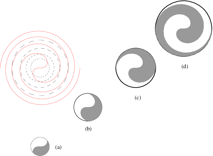
While the first two properties are indisputable, our choice of the third axiom requires some motivation as this condition is often not met in the actual yin-yang design. Say, in the most familiar versions some radii do not cross $\beta$ at all (Fig. 1-a,b). On the other hand, there occur yin-yang patterns where the number of crossings can vary from 1 to 2 (Fig. 1-d). Figure 1-c shows an instance with ( ${\mathcal{A}}_{\ref{ax:rad}}$ ) obeyed, that arose from attempts to explain the origins of the yin-yang symbolism [7, 8].¹¹ 1 The border between Yin and Yang consists of two semicircles in Fig. 1-b and is Archimedes’s spiral in Fig. 1-c; the discussion of Fig. 1-a,d is postponed to Appendix B. All the variations can be treated uniformly if we take a dynamic look at the subject. It will be deduced from our axiomatics that $\beta$ is a spiral. We therefore can consider a continuous family of yin-yang symbols determined by the spiral as shown in Fig. 2. Thus, ( ${\mathcal{A}}_{\ref{ax:rad}}$ ) specifies a single representative that will allow us to expose the whole family.

Refer to caption — Figure 1. A gallery of yin-yang symbols: (a) a clasical version, cf. [12]; (b) a modern version; (c) the version presented in [7, 8]; (c) a Korean flag from 19th century [9].

There is a huge variety of curves satisfying ( ${\mathcal{A}}_{\ref{ax:cong}}$ )–( ${\mathcal{A}}_{\ref{ax:rad}}$ ) and hence an essential further specification is needed. We suggest another axiom, which is both mathematically beautiful and philosophically meaningful. It comes from continuous Ramsey theory.

Let $\Omega$ be a bounded figure of revolution in a Euclidean space. Suppose that $\mu(\Omega)=1$ , where $\mu$ denotes the Lebesgue measure. Consider the set $\mathit{Sym}(\Omega)$ of symmetries of $\Omega$ , i.e., of all space isometries taking $\Omega$ onto itself. Call a set $X\subseteq\Omega$ symmetric if $s(X)=X$ for some non-identity $s\in\mathit{Sym}(\Omega)$ . The density version of a simple Ramsey-type result says that every measurable set $A\subseteq\Omega$ contains a symmetric subset of measure at least $\mu(A)^{2}$ (see our previous work [1], a survey article [2], or an overview in Section 2). For the case that $\Omega$ is the circle in $\mathbb{R}^{2}$ or the sphere or the ball in $\mathbb{R}^{n}$ , $n\geq 3$ , we proved an even stronger fact [1, 2]: If $0<\mu(A)<1$ , then $A\subset\Omega$ always contains a symmetric subset whose measure is strictly more than $\mu(A)^{2}$ .

On the other hand, we discovered a magic difference of the plane disk $\Omega=D$ from the aforementioned figures: it contains a set $A\subset D$ of measure $1/2$ all whose symmetric subsets have measure at most $1/4$ . Let us call such an $A$ perfect. Any perfect set $A$ has a remarkable property: For every axial symmetry $s$ of $D$ , the maximum subset of $A$ symmetric with respect to $s$ has measure $1/4$ . In words admitting far-going esoteric interpretations, perfect sets demonstrate a sharp equilibrium between their “symmetric” and “asymmetric” parts, whatever particular symmetry $s$ is considered. We put this phenomenon in our axiom system.

( ${\mathcal{A}}_{\ref{ax:perf}}$ )

$\beta$ splits $D$ into perfect sets (from now on we suppose that $D$ has unit area).

There is still a lot of various examples of curves satisfying ( ${\mathcal{A}}_{\ref{ax:cong}}$ )–( ${\mathcal{A}}_{\ref{ax:perf}}$ ). Nevertheless, we are able to show that these four axioms determine a unique curve $\beta$ after imposing two other natural conditions.

( ${\mathcal{A}}_{\ref{ax:smooth}}$ )

$\beta$ is smooth, i.e., has an infinitely differentiable parameterization $\beta:[0,1]\rightarrow D$ with nonvanishing derivative.

The other condition expresses a belief that the border between Yin and Yang should be cognizable, i.e., it should not be transcendent neither in the philosophical nor in the mathematical sense.

( ${\mathcal{A}}_{\ref{ax:alg}}$ )

$\beta$ is algebraic in polar coordinates.

By polar coordinates we mean the mapping $\Pi$ from the two-dimensional space of parameters $(\phi,r)$ onto two-dimensional space of parameters $(x,y)$ defined by the familiar relations $x=r\cos\phi$ and $y=r\sin\phi$ . The $(x,y)$ -space is considered the standard Cartesian parameterization of the plane. Note that, like $x$ and $y$ , both $\phi$ and $r$ are allowed to take on any real value. A curve in the $(\phi,r)$ -plane is algebraic if all its points satisfy an equation $P(x,y)=0$ for some bivariate nonzero polynomial $P$ . A curve in the $(x,y)$ -plane is algebraic in polar coordinates if it is the image of an algebraic curve under the mapping $\Pi$ .

A classical instance of a curve both smooth and algebraic in polar coordinates is Fermat’s spiral (exactly this spiral is drown in Fig. 2). Fermat’s spiral is defined by equation $a^{2}r^{2}=\phi$ . Its part specified by the restriction $0\leq\phi\leq\pi$ (or, equivalently, $-\sqrt{\pi}/a\leq r\leq\sqrt{\pi}/a$ ) is inscribed in the disk of area $(\pi/a)^{2}$ .

Theorem 1.1.

Fermat’s spiral $\pi^{2}r^{2}=\phi$ is, up to congruence, a unique curve satisfying the axiom system ( ${\mathcal{A}}_{\ref{ax:cong}}$ )–( ${\mathcal{A}}_{\ref{ax:alg}}$ ).

Thus, if we are willing to accept axioms ( ${\mathcal{A}}_{\ref{ax:cong}}$ )–( ${\mathcal{A}}_{\ref{ax:alg}}$ ), the yin-yang symbol must look as in Fig. 2. Note that the factor of $\pi^{2}$ in the curve equation in Theorem 1.1 comes from the condition that $D$ has area 1. As all Fermat’s spirals are homothetic, we can equally well draw the yin-yang symbol using, say, the spiral $\phi=r^{2}$ . Varying the range of $r$ , we obtain modifications as twisted as desired (see a MetaPost code in Appendix A).

In the next section we overview relevant facts from continuous Ramsey theory. Theorem 1.1 is proved in Section 3. In Section 4 we discuss modifications of the axiom system ( ${\mathcal{A}}_{\ref{ax:cong}}$ )–( ${\mathcal{A}}_{\ref{ax:alg}}$ ). In particular, we show that, after removal of ( ${\mathcal{A}}_{\ref{ax:smooth}}$ ) or ( ${\mathcal{A}}_{\ref{ax:alg}}$ ), the system is not any more categorical, that is, does not specify the line between Yin and Yang uniquely.

2. Density results on symmetric subsets

We have mentioned several Ramsey-type results on symmetric subsets as a source of motivation for ( ${\mathcal{A}}_{\ref{ax:perf}}$ ), the cornerstone of our yin-yang axiomatics. Now we supply some details. Recall that we consider any geometric figure $\Omega\subset\mathbb{R}^{n}$ along with its symmetry group $\mathit{Sym}(\Omega)$ consisting of the isometries of $\mathbb{R}^{n}$ that take $\Omega$ onto itself. Given a measurable set $A\subseteq\Omega$ , we address subsets of $A$ symmetric with respect to a symmetry in $\mathit{Sym}(\Omega)$ and want to know how large they can be. To prove the existence of a large symmetric subset, it sometimes suffices to restrict one’s attention to symmetries in a proper subset of $\mathit{Sym}(\Omega)$ . In the case of the circle we will focus on its axial symmetries. After identification of the circle with the additive group $\mathbb{S}=\mathbb{R}/\mathbb{Z}$ , these symmetries are expressed in the form $s_{g}(x)=g-x$ .

Any figure of revolution $\Omega$ can be represented as the product $\Omega=\mathbb{S}\times\Theta$ for an appropriate $\Theta$ . The Lebesgue measure on $\Omega$ is correspondingly decomposed into $\mu=\lambda\times\nu$ . It is supposed that $\lambda(\mathbb{S})=1$ and $\nu(\Theta)=1$ . Note that the $\Omega$ inherits the reflectional symmetries of $\mathbb{S}$ , namely $s_{g}(x,y)=(g-x,y)$ , where $x\in\mathbb{S}$ and $y\in\Theta$ .

Theorem 2.1 ([1, 2]).

Let $\mathbb{S}\times\Theta$ be a figure of revolution. Then every measurable set $A\subseteq\mathbb{S}\times\Theta$ contains a symmetric subset of measure at least $\mu(A)^{2}$ .

Proof.

For a fixed $y\in\Theta$ , let $A_{y}=\bigl\{\hskip 1.42262ptx\in\mathbb{S}:\hskip 1.42262pt(x,y)\in A\bigr\}$ be the corresponding section of $A$ . By $\chi_{U}$ we denote the characteristic function of a set $U$ . Since $s_{g}$ is involutive, the maximum subset of $A$ symmetric with respect to $s_{g}$ is equal to $A\cap s_{g}A$ . Its measure is representable as

\mu(A\cap s_{g}A)=\int_{\Omega}\chi_{A\cap s_{g}A}(x,y)\,d\mu(x,y)=\int_{\Theta}\int_{\mathbb{S}}\chi_{A_{y}}(x)\chi_{A_{y}}(g-x)\,d\lambda(x)d\nu(y).

Averaging it on $g$ and changing the order of integration, we have

\int_{\mathbb{S}}\mu(A\cap s_{g}A)\,d\lambda(g)=\int_{\Theta}\int_{\mathbb{S}}\chi_{A_{y}}(x)\int_{\mathbb{S}}\chi_{A_{y}}(g-x)\,d\lambda(g)d\lambda(x)d\nu(y)=\int_{\Theta}\lambda(A_{y})^{2}\,d\nu(y).

By the Cauchy-Schwartz inequality,

\int_{\mathbb{S}}\mu(A\cap s_{g}A)\,d\lambda(g)\geq\left(\int_{\Theta}\lambda(A_{y})\,d\nu(y)\right)^{2}=\mu(A)^{2}.

Thus, there must exist a $g\in\mathbb{S}$ such that $\mu(A\cap s_{g}A)\geq\mu(A)^{2}$ . ∎

In some cases Theorem 2.1 admits a non-obvious improvement.

Theorem 2.2 ([1, 2]).

Let $\Omega$ be the circle in $\mathbb{R}^{2}$ or the sphere or the ball in $\mathbb{R}^{k}$ , $k\geq 3$ . Suppose that $A\subset\Omega$ is measurable. If $0<\mu(A)<1$ , then $A$ contains a symmetric subset of measure strictly more than $\mu(A)^{2}$ .

Proof.

We here prove the theorem only for the circle $\mathbb{S}$ . The subsequent argument is hardly applicable to the spheres and balls; the reader is referred to the treatment of these cases in [1, 2].

Denote $f(g)=\mu(A\cap s_{g}A)$ . We will prove that the sharp inequality $f(g)>\mu(A)^{2}$ must occur at least for some $g$ . Assume to the contrary that $f(g)\leq\mu(A)^{2}$ for all $g$ . Applying the averaging argument as in the proof of Theorem 2.1, we obtain $\int_{\mathbb{S}}f(g)\,dg=\mu(A)^{2}$ and, therefore,

f(g)=\mu(A)^{2}\mathrm{\ for\ almost\ all\ }g.

(1)

Let $\chi_{A}(x)=\sum_{n\in\mathbb{Z}}c_{n}e^{2\pi inx}$ be the Fourier expansion of $\chi_{A}$ in $L_{2}(\mathbb{S})$ . Note that $f(g)=\int_{\mathbb{S}}\chi_{A}(x)\chi_{A}(g-x)\,dx$ , that is, $f$ is the convolution $\chi_{A}\star\chi_{A}$ . This allows us to determine the Fourier expansion for $f$ from the Fourier expansion for $\chi_{A}$ , namely

f(g)=\sum_{n\in\mathbb{Z}}c_{n}^{2}e^{2\pi ing}

in $L_{2}(\mathbb{S})$ . On the other hand, we know from (1) that $f$ is almost everywhere equal to a constant (i.e., $f$ is a constant function in $L_{2}(\mathbb{S})$ ). By uniqueness of the Fourier expansion we conclude that $c_{n}^{2}=0$ whenever $n\neq 0$ . It follows that $\chi_{A}(x)=c_{0}$ almost everywhere. This is possible only if $c_{0}=0$ or $c_{0}=1$ , contradictory to the assumption that $0<\mu(A)<1$ . ∎

Somewhat surprisingly, Theorem 2.2 fails to be true for the disk.

Definition 2.3.

Let $D$ denote the disk of unit area. Call a set $A\subset D$ perfect if $\mu(A)=1/2$ and every symmetric subset of $A$ has measure at most $1/4$ .

Analysis of the proof of Theorem 2.2 reveals a remarkable property of perfect sets.

Lemma 2.4.

For every axial symmetry $s_{g}$ of $D$ , the maximum subset of a perfect set $A$ symmetric with respect to $s_{g}$ has measure exactly $1/4$ , i.e.,

\mu(A\cap s_{g}A)=1/4\emph{\ for\ all\ }g.

Proof.

Let $f(g)=\mu(A\cap s_{g}A)$ . The lemma follows from (1) and the continuity of $f$ . We only have to prove the latter.

Given an $\varepsilon>0$ , choose a compact set $K\subset A$ and an open subset $U\subset D$ so that $K\subset A\subset U$ and $\mu(U)-\mu(K)<\varepsilon/2$ . Let $r_{h}$ denote the rotation of $D$ by angle $2\pi h$ . For any $\epsilon>0$ there is a $\delta>0$ such that, if $|h|<\delta$ , then the distance between $r_{h}x$ and $x$ is less than $\epsilon$ for every $x\in D$ . Using this and the compactness of $K$ , we can take $\delta>0$ so small that $r_{h}K\subset U$ whenever $|h|<\delta$ . Let $g^{\prime}=g+h$ . Assuming that $|h|<\delta$ , we have

	$\displaystyle\|f(g^{\prime})-f(g)\|$	$\displaystyle\leq$	$\displaystyle\mu(s_{g^{\prime}}A\setminus s_{g}A)+\mu(s_{g}A\setminus s_{g^{\prime}}A)=\mu(A\setminus r_{h}A)+\mu(A\setminus r_{-h}A)$
		$\displaystyle\leq$	$\displaystyle\mu(U\setminus r_{h}K)+\mu(U\setminus r_{-h}K)=2(\mu(U)-\mu(K))<\varepsilon,$

which witnesses the continuity of $f$ at $g$ . ∎

Theorem 2.5 ([1, 2]).

Perfect sets exist.

We precede the proof of Theorem 2.5 with a technical suggestion, that will be useful also in the next section. Instead of the disk $D$ , it will be practical to deal with the cylinder $C=\mathbb{S}\times(0,1]$ supplied with the product measure $\mu=\lambda\times\lambda$ . For this purpose we prick out the center from $D$ and establish a one-to-one mapping $F:D\rightarrow C$ preserving measure and symmetry. We describe a point in $C$ by a pair of coordinates $(u,v)$ with $0<u\leq 1$ and $0<v\leq 1$ , whereas for $D$ we use polar coordinates $(r,\phi)$ with $0<r\leq\pi^{-1/2}$ and $0<\phi\leq 2\pi$ . In these coordinate systems, we define

F(r,\phi)=(\frac{\phi}{2\pi},\pi r^{2}).

Since $F$ is a diffeomorphism, a set $X\subseteq D$ is measurable iff so is $F(X)$ .

To see the geometric sense of $F$ , notice that this mapping takes a radius of the disk onto a longitudinal section of the cylinder. Furthermore, a concentric circle of $D$ is taken onto a cross section of $C$ so that the area below the section is equal to the area within the circle. It follows that, if a set $X\subseteq D$ is measurable, then $X$ and $F(X)$ have the same measure.

The correspondence $F$ preserves symmetry in the following sense: For every $s\in\mathit{Sym}(D)$ there is an $s^{\prime}\in\mathit{Sym}(C)$ such that, for any $X\subseteq D$ , we have $s(X)=X$ iff $s^{\prime}(F(X))=F(X)$ . Specifically, the rotation $s^{\prime}(u,v)=(u+h,v)$ (resp., the reflection $s^{\prime}(u,v)=(g-u,v)$ ) of the cylinder corresponds to the rotation by angle $2\pi h$ (resp., to the reflection in the diameter $\phi=\pi g$ ) of the disk.

Finally, it will be practical to identify $\mathbb{S}$ with $(0,1]$ and replace $C$ with the square $(0,1]\times(0,1]$ regarded as the development of the cylinder on a plane.

Proof of Theorem 2.5. The argument presented below is different from that used in [1, 2].

Using the transformation $F$ , we prefer to deal with the cylinder $C$ . We will construct a set $A\subset C$ so that $F^{-1}(A)$ is perfect. This goal will be achieved by ensuring the following properties of $A$ :

•

$\mu(A)=1/2$ .
•

$A$ contains no subset symmetric with respect to any rotation.
•

Every subset of $A$ symmetric with respect to a reflection has measure $1/4$ .

Given $v\in(0,1]$ , we will denote $A_{v}=\bigl\{\hskip 1.42262ptu\in\mathbb{S}:\hskip 1.42262pt(u,v)\in A\bigr\}$ . In the course of construction of $A$ we will obey the condition that

\mathbb{S}\setminus A_{v}=A_{v}+\frac{1}{2}

(2)

for every $v$ (i.e., each $A_{v}$ and its centrally symmetric image make up a partition of the circle).

The desired set $A$ will be constructed by parts, first below the cross section $v=1/2$ and then above it. There is much freedom for the first part $A^{\prime}=A\,\cap\,\mathbb{S}\times(0,\frac{1}{2}]$ . We choose it to be an arbitrary set with each slice $A_{v}$ being a continuous semi-interval of length $1/2$ , i.e., a semicircle in $\mathbb{S}$ . The other part $A^{\prime\prime}=A\,\cap\,\mathbb{S}\times(\frac{1}{2},1]$ is obtained by lifting $A^{\prime}$ and rotating it by angle $\pi/2$ , that is, $A^{\prime\prime}=A^{\prime}+(\frac{1}{4},\frac{1}{2})$ . Note that (2) is therewith satisfied. The simplest example of a perfect set obtainable this way is shown in Fig. 3.

It remains to verify that the $A$ has the proclaimed properties. Since each $A_{v}$ is a semicircle, $A$ does not contain any nonempty subset symmetric with respect to a rotation. Consider now a reflection $s_{g}(u,v)=(g-u,v)$ and compute the measure of the maximum subset of $A$ symmetric with respect to $s_{g}$ :

\mu(A\cap s_{g}A)=\int_{0}^{1}\lambda(A_{v}\cap(g-A_{v}))\,dv\\ =\int_{0}^{1/2}\lambda(A_{v}\cap(g-A_{v}))+\lambda((\frac{1}{4}+A_{v})\cap(g-\frac{1}{4}-A_{v}))\,dv.

Note that $\lambda((\frac{1}{4}+A_{v})\cap(g-\frac{1}{4}-A_{v}))=\lambda((\frac{1}{2}+A_{v})\cap(g-A_{v}))$ . Taking into account (2), we conclude that

\mu(A\cap s_{g}A)=\int_{0}^{1/2}\lambda(A_{v}\cap(g-A_{v}))+\lambda((\mathbb{S}\setminus A_{v})\cap(g-A_{v}))\,dv=\int_{0}^{1/2}\lambda(g-A_{v})\,dv=\frac{1}{4}.

The proof is complete. ∎

3. Establishing the borderline between Yin and Yang

Here we prove Theorem 1.1. The proof essentially consists of Lemmas 3.1 and 3.2 and is given in Section 3.1. The proof of Lemma 3.2 is postponed to Section 3.3 with the necessary preliminaries outlined in Section 3.2.

3.1. Proof of Theorem 1.1

Assuming that $\beta$ satisfies axioms ( ${\mathcal{A}}_{\ref{ax:cong}}$ )–( ${\mathcal{A}}_{\ref{ax:rad}}$ ), we take into consideration another curve $\alpha$ associated with $\beta$ in a natural way. It easily follows from ( ${\mathcal{A}}_{\ref{ax:cong}}$ ) and ( ${\mathcal{A}}_{\ref{ax:conc}}$ ) that $\beta$ is symmetric with respect to the center $O$ of the disk $D$ and that $O$ splits $\beta$ into two congruent branches, say, $\beta_{1}$ and $\beta_{2}$ . We will use the transformation $F:D\setminus\{O\}\rightarrow(0,1]^{2}$ described before the proof of Theorem 2.5, where the square $(0,1]^{2}$ is thought of as the development of the cylinder $C=\mathbb{S}\times(0,1]$ . Let $\alpha$ be the image of $\beta_{1}$ under $F$ . By ( ${\mathcal{A}}_{\ref{ax:rad}}$ ), this curve can be considered the graph of a function $v=\alpha(u)$ , where $u$ ranges in a semi-interval of length $1/2$ . Shifting, if necessary, the coordinate system and appropriately choosing the positive direction of the $u$ -axis, we suppose that $\alpha$ is defined for $0<u\leq 1/2$ and hence $\lim_{u\to 0}\alpha(u)=0$ . Since $\beta_{1}$ goes from the center to a peripheral point, we have $\alpha(1/2)=1$ . Since $\beta_{1}$ crosses each concentric circle exactly once, $\alpha$ is a monotonically increasing function. Note that the image of $\beta_{2}$ under $F$ is obtained from $\alpha$ by translation in $1/2$ , that is, it is the graph of the function $v=\alpha(u-1/2)$ on $1/2<u\leq 1$ (see the left square in Fig. 4).

Lemma 3.1.

Suppose that $\beta$ satisfies ( ${\mathcal{A}}_{\ref{ax:cong}}$ )–( ${\mathcal{A}}_{\ref{ax:rad}}$ ) and let $\alpha$ be the associated curve. Then $\beta$ satisfies ( ${\mathcal{A}}_{\ref{ax:perf}}$ ) if and only if

\alpha(u+\frac{1}{4})=\alpha(u)+\frac{1}{2}\mathrm{\ for\ all\ }0<u\leq\frac{1}{4}.

(3)

Proof.

The curve $\alpha$ and its shift in angle $\pi$ split the cylinder $C$ into two congruent parts, say, $A$ and $B$ . Those are the images under $F$ of the two parts into which $D$ is split by $\beta$ .

If (3) holds true, then $A$ can be considered an instance of the general construction described in the proof of Lemma 2.4. It follows that $F^{-1}(A)$ and $F^{-1}(B)$ are perfect sets, that is, ( ${\mathcal{A}}_{\ref{ax:perf}}$ ) is fulfilled.

Conversely, assume ( ${\mathcal{A}}_{\ref{ax:perf}}$ ). Consider the development of the cylinder onto the square and suppose that $A$ is the area in $(0,1]^{2}$ between $\alpha$ and its shift in $1/2$ . Introduce first some notation. Given $v\in(0,1]$ , let $A_{v}=\bigl\{\hskip 1.42262ptu:\hskip 1.42262pt(u,v)\in A\bigr\}$ . Note that $A_{v}$ is the segment with endpoints $\alpha^{-1}(v)$ and $\alpha^{-1}(v)+1/2$ and we can sometimes write $A_{v}=\alpha^{-1}(v)+H$ , where $H=[0,\frac{1}{2}]$ .

Furthermore, denote $\bar{\alpha}(u)=\alpha(u/2)$ , $0<u\leq 1$ , and let $\bar{A}$ be the area of the cylinder $C$ bounded by the graph of $\bar{\alpha}$ and its image under rotation by angle $\pi$ . In the development of $C$ this area looks as shown on the right square in Fig. 4. Given $u\in(0,1]$ , let $\bar{A}_{u}=\bigl\{\hskip 1.42262ptv:\hskip 1.42262pt(u,v)\in\bar{A}\bigr\}$ and $m(u)=\lambda(\bar{A}_{u})$ . If $0<u\leq 1/2$ , we have

\begin{array}[]{rcl}m(u)&=&\bar{\alpha}(u)+(1-\bar{\alpha}(u+\frac{1}{2})),\\[5.69054pt] m(u+\frac{1}{2})&=&\bar{\alpha}(u+\frac{1}{2})-\bar{\alpha}(u).\end{array}

(4)

We are now prepared to prove (3). By ( ${\mathcal{A}}_{\ref{ax:perf}}$ ) and Lemma 2.4, we have

\mu(A\cap s_{g}A)=\frac{1}{4}

for any reflection $s_{g}(u,v)=(g-u,v)$ , where $\mu=\lambda\times\lambda$ is the measure on $(0,1]^{2}$ . Observe that

\lambda(A_{v}\cap s_{g}A_{v})=\lambda((\alpha^{-1}(v)+H)\cap(-\alpha^{-1}(v)+g-H))\\[2.84526pt] =\lambda((2\alpha^{-1}(v)+H)\cap(g-H))=\lambda((\bar{\alpha}^{-1}(v)+H)\cap(g-H))

Suppose that $1/2<g\leq 1$ and continue this chain of equalities:

\lambda(A_{v}\cap s_{g}A_{v})=\int_{g-1/2}^{g}\chi_{\bar{\alpha}^{-1}(v)+H}(u)\,du=\int_{g-1/2}^{g}\chi_{\bar{A}}(u,v)\,du=\int_{g-1/2}^{g}\chi_{\bar{A}_{u}}(v)\,du.

Using it, we obtain

\mu(A\cap s_{g}A)=\int_{0}^{1}\lambda(A_{v}\cap s_{g}A_{v})\,dv=\int_{0}^{1}\int_{g-1/2}^{g}\chi_{\bar{A}_{u}}(v)\,dudv\\ =\int_{g-1/2}^{g}\int_{0}^{1}\chi_{\bar{A}_{u}}(v)\,dvdu=\int_{g-1/2}^{g}m(u)\,du.

Since $\mu(A\cap s_{g}A)$ is a constant function of $g$ , differentiation in $g$ gives us the identity $m(g)-m(g-1/2)=0$ , that is,

m(u)=m(u+\frac{1}{2})\mathrm{\ for\ all\ }0<u\leq\frac{1}{2}.

(5)

Substituting from (4), we get

2\bar{\alpha}(u+\frac{1}{2})=2\bar{\alpha}(u)+1.

In particular, for all $0<u\leq 1/4$ we have

\bar{\alpha}(2u+\frac{1}{2})=\bar{\alpha}(2u)+\frac{1}{2},

which in terms of $\alpha$ is exactly what was claimed. ∎

The simplest curve satisfying (3) is the line $v=2u$ , $0\leq u\leq 1/2$ . As easily seen, under the application of $F^{-1}$ this line and its shift $v=2u-1$ , $1/2\leq u\leq 1$ , are transformed into Fermat’s spiral $\pi^{2}r^{2}=\phi$ , $0\leq\phi\leq\pi$ . It follows that Fermat’s spiral, which clearly satisfies ( ${\mathcal{A}}_{\ref{ax:cong}}$ )–( ${\mathcal{A}}_{\ref{ax:rad}}$ ), also satisfies ( ${\mathcal{A}}_{\ref{ax:perf}}$ ). Note that ( ${\mathcal{A}}_{\ref{ax:smooth}}$ ) and ( ${\mathcal{A}}_{\ref{ax:alg}}$ ) hold true as well: Fermat’s spiral is explicitly given by an algebraic relation in polar coordinates and is smooth, for example, due to parameterization

\left\{\begin{array}[]{lll}x&=&\textstyle\frac{1}{\pi}\,t\cos t^{2},\\[4.2679pt] y&=&\textstyle\frac{1}{\pi}\,t\sin t^{2}.\end{array}\right.

To prove Theorem 1.1, we hence have to prove that, if a curve $\beta$ satisfies ( ${\mathcal{A}}_{\ref{ax:cong}}$ )–( ${\mathcal{A}}_{\ref{ax:alg}}$ ), then it coincides, up to congruence, with Fermat’s spiral. It suffices to prove that the associated curve $\alpha$ is a straight line segment.

Since $\beta$ is smooth by ( ${\mathcal{A}}_{\ref{ax:smooth}}$ ) and $\alpha$ is a smooth transformation of a part of $\beta$ , we conclude that $\alpha$ is smooth as well. As follows from ( ${\mathcal{A}}_{\ref{ax:alg}}$ ) and the definition of transformation $F$ , all points of $\alpha$ satisfy relation $P(u,\sqrt{v})=0$ for a nonzero bivariate polynomial $P$ . Since this relation can be rewritten in the form $\sqrt{v}\,Q(u,v)+R(u,v)=0$ for some polynomials $Q$ and $R$ , the points of $\alpha$ satisfy polynomial relation $v\,Q^{2}(u,v)-R^{2}(u,v)=0$ .

Thus, $\alpha$ is a smooth algebraic curve. By Lemma 3.1, $\alpha$ satisfies relation (3). This means that $\alpha$ has infinite intersection with its shift $\alpha+(\frac{1}{4},\frac{1}{2})$ . Theorem 1.1 immediately follows from the following fact.

Lemma 3.2.

If a smooth algebraic curve $\gamma\subset\mathbb{R}^{2}$ has infinite intersection with its shift in a nonzero vector $(a,b)$ , then $\gamma$ is contained in a line.

The proof of Lemma 3.2 takes the rest of this section.

3.2. Background on smooth algebraic curves

In what follows we suppose that a curve $\gamma\subset\mathbb{R}^{2}$ is the image of a real interval under an injective continuous map (the forthcoming considerations apply to $\alpha$ , which is the image of a semi-interval, after removal from $\alpha$ its endpoint). Recall that $\gamma$ is smooth if it has an infinitely differentiable parameterization $\gamma:(0,1)\rightarrow\mathbb{R}^{2}$ with nonvanishing derivative. A $\gamma$ is algebraic if every point $(x,y)\in\gamma$ satisfies relation $P(x,y)=0$ for a nonzero polynomial $P$ with real coefficients. The degree of $\gamma$ is the minimum possible degree of such a $P$ . If $P$ is irreducible, i.e., does not admit factorization $P(x,y)=Q(x,y)R(x,y)$ with $Q$ and $R$ both being nonconstant real polynomials, then $\gamma$ is called irreducibly algebraic.

Theorem 3.3 (Bézout, see, e.g., [5]).

Suppose that $P_{1}$ and $P_{2}$ are distinct bivariate polynomials of degree $m$ and $n$ , respectively. Let $\rho_{i}=\bigl\{\hskip 1.42262pt(x,y)\in\mathbb{R}^{2}:\hskip 1.42262ptP_{i}(x,y)=0\bigr\}$ , $i=1,2$ . If both $P_{1}$ and $P_{2}$ are irreducible, then $\rho_{1}$ and $\rho_{2}$ have at most $mn$ points in common.

A function $f:\mathbb{R}\rightarrow\mathbb{R}$ (resp., $f:\mathbb{C}\rightarrow\mathbb{C}$ ) is called analytic at point $x_{0}$ if in some neighborhood of $x_{0}$ the function develops in a power series

f(x)=\sum_{n=0}^{\infty}a_{n}(x-x_{0})^{n}

with real (resp., complex) coefficients $a_{n}$ . Furthermore, we call $f$ analytic on an open set $U$ if it is analytic at every $x_{0}\in U$ . It can be showed that, if $f$ is analytic at a point $x_{0}$ , then it is analytic on a neighborhood of $x_{0}$ . The following noticeable fact applies to both real and complex analytic functions.

Theorem 3.4 (The Uniqueness Theorem, see, e.g., [6]).

Let functions $f$ and $g$ be analytic on a connected set $U$ . Suppose that the set $\bigl\{\hskip 1.42262ptx\in U:\hskip 1.42262ptf(x)=g(x)\bigr\}$ has an accumulation point inside $U$ . Then $f(x)=g(x)$ everywhere on $U$ .

We will need also the following result.

Theorem 3.5 ([4]).

Let $P(z,w)$ be a bivariate complex polynomial that essentially depends on $w$ . Suppose that $P(0,0)=0$ . Then there are a positive integer $m$ and complex functions $f_{1}(z),\dots,f_{k}(z)$ analytic on a neighborhood of zero $U\subset\mathbb{C}$ such that, for each nonnegative real $t\in U$ , every root of the univariate polynomial $P(t,\cdot)$ in $U$ is equal to $f_{i}(\kern-2.0pt\sqrt[m]{t})$ for some $i\leq k$ .

Finally, we introduce a useful concept stronger than that of a smooth curve. We call a curve $\gamma\subset\mathbb{R}^{2}$ analytic if for each point $(x_{0},y_{0})\in\gamma$ we can choose a Cartesian coordinate system so that, within a neighborhood of $(x_{0},y_{0})$ , the curve $\gamma$ becomes the graph of a real function $y=f(x)$ analytic at $x_{0}$ .

3.3. Proof of Lemma 3.2

We begin with a simpler particular case. Assume that $\gamma$ is irreducibly algebraic.

Let $P(x,y)$ be an irreducible polynomial such that $\gamma\subseteq\rho$ where $\rho=\{(x,y)\in\mathbb{R}^{2}\,:\,P(x,y)=0\}$ . Note that $\rho+(a,b)=\bigl\{\hskip 1.42262pt(x,y)\in\mathbb{R}^{2}:\hskip 1.42262ptP(x-a,y-b)=0\bigr\}$ and that the polynomial $P(x-a,y-b)$ is irreducible as well. Since the intersection $\rho\cap(\rho+(a,b))\supseteq\gamma\cap(\gamma+(a,b))$ is infinite, the Bézout Theorem implies equality $\rho=\rho+(a,b)$ . It follows that $\rho$ has infinite intersection with line $\ell=\bigl\{\hskip 1.42262pt(x,y)\in\mathbb{R}^{2}:\hskip 1.42262ptb(x-x_{0})-a(y-y_{0})=0\bigr\}$ for an arbitrary $(x_{0},y_{0})\in\rho$ . Since any linear polynomial is irreducible, we can apply the Bézout Theorem once again and conclude that $\ell=\rho\supset\gamma$ .

To prove Lemma 3.2, it now suffices to show that every smooth algebraic curve is irreducibly algebraic. We split this task into two steps by proving first that every smooth algebraic curve is analytic and then that every analytic algebraic curve is irreducibly algebraic. The rest of the proof of Lemma 3.2 consists of the two respective lemmas.

Lemma 3.6.

Every smooth algebraic curve is analytic.

Proof.

Let $(x(s),y(s))$ , $0<s<1$ , be a smooth algebraic curve. We need to check that it is analytic at each point $s_{0}\in(0,1)$ . We lose no generality assuming that $x(s_{0})=y(s_{0})=0$ . By a suitable rotation of the coordinate system, we can reduce our problem to the case that in some neighborhood of $(0,0)$ the curve coincides with the graph of a $C^{\infty}$ -function $y(x)$ defined on an interval $(-\delta,\delta)$ . It suffices to verify that the function $y(x)$ is analytic at zero.

In fact, it suffices to find $\varepsilon>0$ and two power series $\sum_{n=0}^{\infty}a_{n}x^{n}$ and $\sum_{n=0}^{\infty}b_{n}x^{n}$ that converge to the function $y(x)$ on the intervals $[0,\varepsilon)$ and $(-\varepsilon,0]$ respectively. Indeed, one can use standard analytic tools to show that

a_{n}=\frac{y^{(n)}(0)}{n!}=b_{n},

(6)

which means that the two series determine the same analytic function coinciding with $y(x)$ on $(-\varepsilon,\varepsilon)$ .

Now we show how to find $\varepsilon$ and the series $\sum_{n=0}^{\infty}a_{n}x^{n}$ (the series $\sum_{n=0}^{\infty}b_{n}x^{n}$ exists by a symmetric argument).

Since our smooth curve $(x,y(x))$ is algebraic, there is a polynomial $P(x,y)$ such that $P(x,y(x))=0$ for all $x\in(-\delta,\delta)$ . Note that $P$ must contain at least one occurrence of the variable $y$ . Let a neighborhood $U\subset\mathbb{C}$ of zero, functions $f_{1},\ldots,f_{k}$ analytic on $U$ , and a positive integer $m$ be as granted by Theorem 3.5. Suppose that the $f_{i}$ ’s are pairwise distinct. Take a positive real $\varepsilon<\delta$ so small that $\bigl\{\hskip 1.42262pt(x,y(x)):\hskip 1.42262pt|x|<\varepsilon\bigr\}\subset U^{2}$ and

f_{i}(z)\neq f_{j}(z)\mathrm{\ whenever\ }0<|z|<\sqrt[m]{\varepsilon},

(7)

for any $1\leq i<j\leq k$ . Such a choice of $\varepsilon$ exists by the Uniqueness Theorem. Non-equality (7) ensures disjointness of sets

W_{i}=\bigl\{\hskip 1.42262pt(x,f_{i}(\kern-2.0pt\sqrt[m]{x})):\hskip 1.42262pt0<x<\varepsilon\bigr\}\mathrm{\ and\ }W_{j}=\bigl\{\hskip 1.42262pt(x,f_{j}(\kern-2.0pt\sqrt[m]{x})):\hskip 1.42262pt0<x<\varepsilon\bigr\}.

By Theorem 3.5 we have inclusion $\bigl\{\hskip 1.42262pt(x,y(x)):\hskip 1.42262pt0<x<\varepsilon\bigr\}\subset\bigcup_{i=1}^{k}W_{i}$ . It follows by continuity of the graph of $y(x)$ that

\bigl\{\hskip 1.42262pt(x,y(x)):\hskip 1.42262pt0<x<\varepsilon\bigr\}\subset W_{i}

(8)

for some $i$ . Develop the analytic function $f_{i}$ into the Maclaurin series $f_{i}(x)=\sum_{n=0}^{\infty}a_{n}x^{n}$ . Replacing, if necessary, the number $\varepsilon$ by a smaller one, we can assume that this series converges to $f_{i}(x)$ uniformly on the interval $[0,\kern-2.0pt\sqrt[m]{\varepsilon})$ . By (8) we hence have $y(x)=\sum_{n=0}^{\infty}a_{n}x^{n/m}$ , where the series converges uniformly for all $x\in[0,\varepsilon)$ . The smoothness of $y(x)$ at zero guarantees that $a_{n}=0$ for all numbers $n$ , not divisible by $m$ . Therefore, $y(x)=\sum_{n=0}^{\infty}a_{nm}x^{n}$ for $x\in[0,\varepsilon)$ , quod erat demonstrandum. It remains to note that the coefficients actually must be real (say, by (6)). ∎

Lemma 3.7.

Every analytic algebraic curve $\gamma\subset\mathbb{R}^{2}$ is irreducibly²² 2 The lemma claims the irreducibility over $\mathbb{R}$ . The proof actually implies the irreducibility even over $\mathbb{C}$ . algebraic.

Proof.

Let $P(x,y)$ be a nonzero polynomial of the smallest possible degree such that $\gamma\subseteq\bigl\{\hskip 1.42262pt(x,y)\in\mathbb{R}^{2}:\hskip 1.42262ptP(x,y)=0\bigr\}$ . We will prove that $P(x,y)$ is irreducible.

Assume to the contrary that $P(x,y)=P_{1}(x,y)P_{2}(x,y)$ with $P_{1}$ and $P_{2}$ being non-constant polynomials. For $i=1,2$ let $\gamma_{i}=\bigl\{\hskip 1.42262pt(x,y)\in\gamma:\hskip 1.42262ptP_{i}(x,y)=0\bigr\}$ and $\gamma_{i}^{\prime}$ be the set of non-isolated points of $\gamma_{i}$ . It is clear that the sets $\gamma_{i}$ and $\gamma_{i}^{\prime}$ are closed in $\gamma$ . We claim that $\gamma_{i}^{\prime}$ is also open in $\gamma$ .

Indeed, take an arbitrary point $(x_{0},y_{0})\in\gamma_{i}^{\prime}$ . After moving appropriately the coordinate system, we can assume that in some neighborhood of $(x_{0},y_{0})$ the curve $\gamma$ coincides with the graph of a real function $f(x)$ analytic on an interval $(x_{0}-\varepsilon,x_{0}+\varepsilon)$ . Notice that the function $g_{i}(x)=P_{i}(x,f(x))$ is analytic on the same interval. Denote the projection of $\gamma_{i}$ onto the $x$ -axis by $\eta_{i}$ . Since $(x_{0},y_{0})\in\gamma_{i}^{\prime}$ , the set $\eta_{i}\cap(x_{0}-\varepsilon,x_{0}+\varepsilon)$ is infinite and contains $x_{0}$ as an accumulation point. By the Uniqueness Theorem, $g_{i}(x)=0$ for all $x\in(x_{0}-\varepsilon,x_{0}+\varepsilon)$ . Consequently, $\bigl\{\hskip 1.42262pt(x,f(x)):\hskip 1.42262ptx_{0}-\varepsilon<x<x_{0}+\varepsilon\bigr\}\subset\gamma_{i}$ and hence $(x_{0},y_{0})$ belongs to the interior of $\gamma_{i}^{\prime}$ in $\gamma$ .

Thus, both the sets $\gamma_{1}^{\prime}$ and $\gamma_{2}^{\prime}$ are closed-and-open in $\gamma$ . Since $\gamma=\gamma_{1}^{\prime}\cup\gamma_{2}^{\prime}$ , one of the sets is nonempty and hence coincides with $\gamma$ by connectedness of $\gamma$ . We see that $\gamma=\gamma_{i}$ is included in $\bigl\{\hskip 1.42262pt(x,y)\in\mathbb{R}^{2}:\hskip 1.42262ptP_{i}(x,y)=0\bigr\}$ for the respective $i$ . This makes a contradiction because $P_{i}$ has degree strictly less than the degree of $P$ . ∎

4. Modifications of the axiom system ( ${\mathcal{A}}_{\ref{ax:cong}}$ )–( ${\mathcal{A}}_{\ref{ax:alg}}$ )

We now investigate what happens when we deviate a little from our axiomatics. In particular, we prove that if either ( ${\mathcal{A}}_{\ref{ax:smooth}}$ ) or ( ${\mathcal{A}}_{\ref{ax:alg}}$ ) is removed, the yin-yang borderline is not specified any more uniquely by the relaxed axiom system. We also discuss modifications of ( ${\mathcal{A}}_{\ref{ax:rad}}$ ) and obtain an existence and uniqueness result under the condition that $\beta$ crosses each radius exactly twice: then any spiral satisfying the other axioms is congruent to the two-turn Fermat spiral.

4.1. Non-algebraic, analytic Yin-Yang variations

The following example demonstrates that there is a variety of non-congruent curves $\beta$ satisfying axioms ( ${\mathcal{A}}_{\ref{ax:cong}}$ )–( ${\mathcal{A}}_{\ref{ax:smooth}}$ ). By Theorem 1.1, all such curves excepting Fermat’s spiral fail to meet ( ${\mathcal{A}}_{\ref{ax:alg}}$ ).

Example 4.1.

Let $0<\lambda<1/4$ . The polar equation

\pi^{2}r^{2}=\phi+\lambda\sin 4\phi,\mathrm{\ where\ }0\leq\phi\leq\pi\ (\mathrm{or\ }-\pi^{-1/2}\leq r\leq\pi^{-1/2}),

(9)

determines an analytic curve $\beta$ satisfying ( ${\mathcal{A}}_{\ref{ax:cong}}$ )–( ${\mathcal{A}}_{\ref{ax:smooth}}$ ).

Proof.

For each $0<\lambda<1/4$ , the function $\rho(\phi)=\phi+\lambda\sin 4\phi$ is strictly monotone and hence invertible. Since $\rho(\phi)$ is analytic, its inverse $\phi=\phi(\rho)$ is analytic as well. This suggests the following analytic parameterization for $\beta$ :

\left\{\begin{array}[]{rcl}x(r)&=&r\cos\phi(\pi^{2}r^{2}),\\ y(r)&=&r\sin\phi(\pi^{2}r^{2}).\end{array}\right.

(10)

Note that $\beta$ is inscribed in the disk of unit area. $\beta$ satisfies ( ${\mathcal{A}}_{\ref{ax:cong}}$ ) because (9) is centrally symmetric. ( ${\mathcal{A}}_{\ref{ax:conc}}$ ) follows from the monotonicity of $\rho(\phi)$ . Furthermore, ( ${\mathcal{A}}_{\ref{ax:rad}}$ ) follows from the fact that $\beta$ is exactly one turn of a spiral. To verify ( ${\mathcal{A}}_{\ref{ax:perf}}$ ), apply the map $F(r,\phi)=(\frac{\phi}{2\pi},\pi r^{2})$ converting the disk into the cylinder. Then $\beta$ is transformed into two curves, one being the graph of function

\alpha(u)=2\,u+\frac{\lambda}{\pi}\,\sin 8\pi u.

Since $\alpha$ satisfies (3), property ( ${\mathcal{A}}_{\ref{ax:perf}}$ ) immediately follows from Lemma 3.1. ( ${\mathcal{A}}_{\ref{ax:smooth}}$ ) is true because the parameterization (10) is analytic and hence smooth. Finally, $\beta$ is an analytic curve because (10) allows us to locally express $y$ as an analytic function of $x$ or $x$ as an analytic function of $y$ . ∎

4.2. Finitely differentiable, algebraic Yin-Yang variations

Now we exhibit non-congruent curves satisfying ( ${\mathcal{A}}_{\ref{ax:cong}}$ )–( ${\mathcal{A}}_{\ref{ax:perf}}$ ) and ( ${\mathcal{A}}_{\ref{ax:alg}}$ ) and being differentiable any preassigned number of times.

Example 4.2.

Let $\lambda$ be a positive real and $k$ a nonnegative integer. Define a function

f(u)=\left\{\begin{array}[]{lr}f_{1}(u)=2u+\lambda u^{k+1}(\frac{1}{4}-u)^{k+1},&\quad 0\leq u\leq\frac{1}{4},\\[5.69054pt] f_{2}(u)=\frac{1}{2}+f_{1}(u-\frac{1}{4}),&\quad\frac{1}{4}\leq u\leq\frac{1}{2}.\end{array}\right.

For each sufficiently small $\lambda$ , the polar equation

\pi r^{2}=f\left(\frac{\phi}{2\pi}\right),\mathrm{\ where\ }0\leq\phi\leq\pi\ (\mathrm{or\ }-\pi^{-1/2}\leq r\leq\pi^{-1/2}),

(11)

determines a $k$ times continuously differentiable curve $\beta$ satisfying axioms ( ${\mathcal{A}}_{\ref{ax:cong}}$ )–( ${\mathcal{A}}_{\ref{ax:perf}}$ ) and ( ${\mathcal{A}}_{\ref{ax:alg}}$ ).

Proof.

Let $\lambda$ be so small that $f_{1}$ has positive derivative on $[0,\frac{1}{4}]$ . As easily seen, $f$ is strictly monotone and hence invertible. Note that $f$ is $k$ times continuously differentiable. A little care is needed only at $u=1/4$ , where we have

f_{1}^{(i)}(1/4)=f_{0}^{(i)}(1/4)=f_{2}^{(i)}(1/4)

for $i\leq k$ and $f_{0}(u)=2u$ . It follows that the inverse $f^{-1}$ is $k$ times continuously differentiable as well. This leads to a $C^{k}$ -parameterization of (11):

\left\{\begin{array}[]{lcl}x(r)&=&r\cos\left(2\pi f^{-1}(\pi r^{2})\right),\\ y(r)&=&r\sin\left(2\pi f^{-1}(\pi r^{2})\right),\end{array}\right.

where $-1/\sqrt{\pi}\leq r\leq 1/\sqrt{\pi}$ .

Axioms ( ${\mathcal{A}}_{\ref{ax:cong}}$ )–( ${\mathcal{A}}_{\ref{ax:rad}}$ ) are easy to verify. The transformation $F$ of the disk into the cylinder takes the branch of (11) for positive $r$ onto the graph of the function $v=f(u)$ . Since $f$ is defined so that $f(u+\frac{1}{4})=f(u)+\frac{1}{2}$ for all $0\leq u\leq\frac{1}{4}$ , axiom ( ${\mathcal{A}}_{\ref{ax:perf}}$ ) follows by Lemma 3.1. Finally, $\beta$ is algebraic because its points satisfy relation

\left(\pi r^{2}-f_{1}(\frac{\phi}{2\pi})\right)\left(\pi r^{2}-f_{2}(\frac{\phi}{2\pi})\right)=0

in polar coordinates. ∎

4.3. Varying the number of radial crossings

For the purpose of the current discussion, we will call a curve $\beta$ spiral if it is described by a polar equation

|r|=f(\phi),\qquad 0\leq\phi\leq\pi\ell,

(12)

where $f$ is a strictly increasing real function. We will say that $\beta$ makes $\ell$ turns, where $\ell$ does not need be integer.

Let $D$ be the disk of unit area centered at the coordinate origin. We will suppose that

f(\pi\ell)=\frac{1}{\sqrt{\pi}}.

(13)

Thus, $\beta$ is inscribed in $D$ and splits $D$ into two parts. Since $\beta$ is symmetric with respect to the origin, we have ( ${\mathcal{A}}_{\ref{ax:cong}}$ ). Condition ( ${\mathcal{A}}_{\ref{ax:conc}}$ ) follows from the monotonicity of $f$ . Axiom ( ${\mathcal{A}}_{\ref{ax:rad}}$ ) captures the case that $\beta$ makes exactly one turn. Consider the following modification:

( ${\mathcal{A^{\prime}}}_{\ref{ax:rad}}$ )

$\beta$ crosses each radius of $D$ twice (besides the center of $D$ ).

As easily seen, any spiral satisfying ( ${\mathcal{A^{\prime}}}_{\ref{ax:rad}}$ ) makes presisely 2 turns. Note that a curve satisfying ( ${\mathcal{A^{\prime}}}_{\ref{ax:rad}}$ ) is not necessary a spiral (see Fig. 5).

Theorem 4.3.

A spiral $\beta$ satisfies the axiom system ( ${\mathcal{A}}_{\ref{ax:cong}}$ )–( ${\mathcal{A}}_{\ref{ax:alg}}$ ) with ( ${\mathcal{A^{\prime}}}_{\ref{ax:rad}}$ ) in place of ( ${\mathcal{A}}_{\ref{ax:rad}}$ ) if and only if it is congruent to Fermat’s spiral

2\pi^{2}r^{2}=\phi,\qquad 0\leq\phi\leq 2\pi.

(14)

The corresponding version of the yin-yang symbol can be seen in Fig. 2-d.

Proof.

We proceed similarly to the proof of Theorem 1.1. Let $\alpha$ be the curve associated with $\beta$ in the way described in the beginning of Section 3.1. We identify this curve with a monotone map $\alpha:(0,1]\rightarrow(0,1]$ . Assume that $\beta$ satisfies ( ${\mathcal{A}}_{\ref{ax:perf}}$ ). The proof of Lemma 3.1 applies and gives us the relation (5), which in terms of $\alpha$ reads

\frac{1}{2}+\alpha(u)+\alpha(u+\frac{1}{2})=\alpha(u+\frac{1}{4})+\alpha(u+\frac{3}{4})\mathrm{\ for\ all\ }0<u\leq\frac{1}{4}.

(15)

Define a function $\sigma:(0,\frac{3}{4}]\rightarrow(0,1]$ by

\sigma(u)=\alpha(u+\frac{1}{4})-\alpha(u).

Relation (15) can be now rewritten as

\sigma(u+\frac{1}{2})=\frac{1}{2}-\sigma(u)\mathrm{\ for\ all\ }0<u\leq\frac{1}{4}.

(16)

Note that $\sigma$ is smooth because so is $\alpha$ . Furthermore, recall that a function $v(u)$ is called algebraic if for some bivariate nonzero polynomial $P$ we have $P(u,v(u))=0$ for all arguments $u$ . It is known that the difference of two algebraic functions is algebraic itself. Thus, $\sigma$ is algebraic because so is $\alpha$ .

We now need the following analog of Lemma 3.2: A smooth algebraic function $\sigma$ satisfies (16) only if $\sigma$ is constant. By Lemmas 3.6 and 3.7, it suffices to prove this claim for an irreducibly algebraic $\sigma$ . Let $P$ be an irreducible polynomial such that $P(u,\sigma(u))=0$ for all $0<u\leq 3/4$ and denote $\rho=\bigl\{\hskip 1.42262pt(u,v):\hskip 1.42262ptP(u,v)=0\bigr\}$ . Consider an affine transformation $S(u,v)=(u+\frac{1}{2},\frac{1}{2}-v)$ . Note that $S(\rho)$ consists of exactly those points $(u,v)$ satisfying $P(u-\frac{1}{2},\frac{1}{2}-v)=0$ . Since polynomials $P(u,v)$ and $P(u-\frac{1}{2},\frac{1}{2}-v)$ are irreducible simultaneously and the intersection $\rho\cap S(\rho)$ is infinite by (16), we conclude by Bézout’s theorem that $\rho=S(\rho)$ . It follows that $\rho=S^{2}(\rho)$ . The latter equality implies that, along with each point $(u_{0},v_{0})$ , the set $\rho$ contains every point $(u_{0}+n,v_{0})$ for a natural $n$ . Therefore, $\rho$ has infinite intersection with the set of points satisfying a linear equation $v-v_{0}=0$ . Applying Bézout’s theorem once again, we see that $\sigma(u)=v_{0}$ everywhere.

We have just proved that

\alpha(u+\frac{1}{4})=\alpha(u)+v_{0}\mathrm{\ for\ all\ }0<u\leq\frac{1}{4},

which provides us with an analog of (3). Applying Lemma 3.2, we conclude that $\alpha$ is a line and, therefore, $\beta$ is Fermat’s spiral.

Verification of conditions ( ${\mathcal{A}}_{\ref{ax:cong}}$ )–( ${\mathcal{A}}_{\ref{ax:alg}}$ ) for Fermat’s spiral (14) is easy and left to the reader. ∎

4.4. Questions and comments

1. Is the axiom system ( ${\mathcal{A}}_{\ref{ax:cong}}$ )–( ${\mathcal{A}}_{\ref{ax:alg}}$ ) with ( ${\mathcal{A^{\prime}}}_{\ref{ax:rad}}$ ) in place of ( ${\mathcal{A}}_{\ref{ax:rad}}$ ) categorical, that is, does it determine Fermat’s spiral uniquely? By Theorem 4.3, if these axioms are fulfilled for another curve, the latter is not a spiral and looks like Fig. 5.

2. Does the axiom system ( ${\mathcal{A}}_{\ref{ax:cong}}$ )–( ${\mathcal{A}}_{\ref{ax:alg}}$ ) remain categorical after exclusion of ( ${\mathcal{A}}_{\ref{ax:conc}}$ ) from it?

3. As we mentioned, any spiral (in the sense of (12)–(13)) has properties ( ${\mathcal{A}}_{\ref{ax:cong}}$ ) and ( ${\mathcal{A}}_{\ref{ax:conc}}$ ). The following hypothesis seems plausible: If a spiral satisfies also axioms ( ${\mathcal{A}}_{\ref{ax:perf}}$ )–( ${\mathcal{A}}_{\ref{ax:alg}}$ ), then it is congruent to Fermat’s spiral with integer number of turns. We can confirm this hypothesis for spirals making at most 2 turns. Consider, for example, the case that a spiral $\beta$ makes $3/2$ turns and show that such a $\beta$ cannot satisfy all conditions ( ${\mathcal{A}}_{\ref{ax:perf}}$ )–( ${\mathcal{A}}_{\ref{ax:alg}}$ ) simultaneously.

If $\beta$ satisfies ( ${\mathcal{A}}_{\ref{ax:perf}}$ ), then for the corresponding function $\alpha:(0,\frac{3}{4}]\rightarrow(0,1]$ we derive from (5), which holds true for any spiral, a relation

\alpha(u)+\alpha(u+\frac{1}{2})=\alpha(u+\frac{1}{4})+\frac{1}{2}\mathrm{\ for\ all\ }0<u\leq\frac{1}{4}.

(17)

If $\beta$ satisfies also ( ${\mathcal{A}}_{\ref{ax:smooth}}$ ) and ( ${\mathcal{A}}_{\ref{ax:alg}}$ ), $\alpha(u)$ must be analytic. Using (17), we can analytically extend this function to a larger interval, say, $(-1/4,1)$ . Differentiating repeatedly (17), we obtain a relation

\alpha^{(k)}(u)+\alpha^{(k)}(u+\frac{1}{2})=\alpha^{(k)}(u+\frac{1}{4})\mathrm{\ for\ all\ }-\frac{1}{4}<u<\frac{1}{2}

(18)

for all $k$ . Substituting $u=0$ and $u=1/4$ in (18), we easily infer equality

\alpha^{(k)}(3/4)=-\alpha^{(k)}(0).

It follows that two analytic functions $\alpha(u)$ and $-\alpha(u-3/4)$ coincide in a neighborhood of the point $u=3/4$ . By the Uniqueness theorem, we have identity $\alpha(u)=-\alpha(u-3/4)$ . Using it in the same way as the identity (16) was used in the proof of Theorem 4.3, we conclude that $\alpha(u)$ must be constant. This contradicts the fact that $\alpha(u)$ is strictly monotone.

4. 3-part yin-yang symbols are frequently seen in Korea, where they are called Sam-Taegeuk, and in Zen temples in the Himalayas, where they are called Gankyil or Wheel of Joy (see Fig. 6-a). The Gankyil has a 4-part variant [3]. From the mathematical point of view, a $k$ -part yin-yang symbol is a partition of the unit disk $D$ by a $k$ -coil spiral into $k$ congruent parts. Equivalently, we can speak of a 1-coil spiral $\sigma$ along with its rotations in angles $2\pi i/k$ for all $i<k$ . Recall that the notion of a spiral was formally introduced in the beginning of Section 4.3; 1 coil means that only positive values of $r$ are allowed, 1 turn means that $0\leq\phi\leq\pi$ . Extending the notion of a perfect set to any measurable set $A\subset D$ , we call $A$ perfect if every symmetric subset of $A$ has measure at most $\mu(A)^{2}$ (symmetric subsets of measure at least $\mu(A)^{2}$ always exist by Theorem 2.1). We adopt our axiomatics in the $k$ -partite case by requiring that each part of the symbol is perfect and that $\sigma$ is smooth and algebraic in polar coordinates. Our main result, Theorem 1.1, generalizes to the $k$ -partite case as follows: Among 1-turn spirals, only Fermat’s spiral meets the postulated conditions (see Fig. 6-b,c).

Acknowledgment

We thank Igor Chyzhykov for referring us to the book [4] and Maria Korolyuk for useful comments.

References

[1] T. Banakh, Ya. Vorobets, and O. Verbitsky. Ramsey-type problems for spaces with symmetry. Izvestiya RAN, seriya matematicheskaya 64(6):3–40 (2000). In Russian. English translation in: Russian Academy of Sciences. Izvestiya. Mathematics 64(6):1091–1127 (2000).
[2] T. Banakh, Ya. Vorobets, and O. Verbitsky. A Ramsey treatment of symmetry. The Electronic Journal of Combinatorics 7(#R52):1–25 (2000).
[3] R. Beer. The Handbook of Tibetan Buddhist Symbols. Serindia Publications, Inc. (2003).
[4] B.A. Fuks, V.I. Levin. Functions of a complex variable and their applications. GITTL, Moscow (1951). In Russian. English translation: Functions of a complex variable and some of their applications II. Pergamon Press, Oxford, and Addison-Wesley, Reading, MA (1961).
[5] F. Kirwan. Complex algebraic curves. Cambridge University Press (1992).
[6] R. Narasimhan, Y. Nievergelt. Complex analysis in one variable. Springer Verlag (2001).
[7] M. Shackelford. The T’ai Chi and the cycle of Chinese months. An online publication, www.fengshui-magazine.com/Trigrams.htm, accessed 9 February 2009.
[8] A. Tsai. Where does the Yin Yang symbol come from? An online publication, www.chinesefor tunecalendar.com/yinyang.htm, accessed 9 February 2009.
[9] The earliest surviving depiction of the flag of Korea, as published in a U.S. Navy book Flags of Maritime Nations in July 1882. Reproduced in: Wikimedia Commons, http://en.wikipedia.org/wiki/Image:Taegukgi.jpg, accessed 9 February 2009.
[10] A drawing of a flag of Korea’s Chosun Dynasty published in the Japanese newspaper Jijishinpo on October 10, 1882. Reprinted in: The Chosun Ilbo, January 26, 2004. http://english.chosun.com/w21data/html/news/200401/200401260030.html, accessed 9 February 2009.
[11] Sam-Taegeuk. An image from the Wikimedia Commons, http://en.wikipedia.org/wiki/File: Sam Taeguk.jpg#file, accessed 9 February 2009. Author: Craig Nagy, http://www.flickr.com/ photos/nagy/. The image is licensed under Creative Commons Attribution 2.0 License http://creativecommons.org/licenses/by/2.0/
[12] Yin-yang. Article in The New Encyklopædia Britannica, 15-th edition. Micropædia, Vol. 12, page 845 (1991).

Appendix A A MetaPost code for drawing yin-yang symbols


beginfig(1)

                     % INPUT PARAMETERS
turn = 1;            % number of turns (does not need to be integer)
radius = 2cm;        % radius of the disk
rotate = 0;          % optional rotation counter-clockwise (degrees)
w = 1bp;             % thickness of the circle
color dark;          % color of the dark part
dark = .5white;      % (1white=white, 0white=black)
boolean clockwise;   % orientation
clockwise = true;    % set to false if counter-clockwise preferred

a = ((.5-turn)*180)+rotate;
shif = (radius+1cm); pair shft; shft = (shif,shif);
if (turn > 2) : interpol = (1/(16turn)) else  : interpol = (1/16) fi;

path spiral;
spiral := (0,0)
 for r:=0 step interpol until 1:
  ..(r,0) rotated (180r*r*turn)
  endfor
 ..(1,0) rotated (180turn);

picture symbol;

symbol = image(
  draw spiral scaled radius;
  draw spiral scaled radius rotated 180;
  draw fullcircle scaled (2radius) withpen pencircle scaled w;
  fill buildcycle(reverse spiral scaled radius rotated 180,
                  spiral scaled radius,
                  halfcircle scaled (2radius) rotated (180*(turn-1)))
                                                   withcolor dark; );

if clockwise:
 draw symbol rotated a shifted shft;
else:
 draw symbol reflectedabout ((0,0),(0,1)) rotated a shifted shft;
fi;

endfig; end

Appendix B Appearances of Fermat’s spiral
in the yin-yang symbolism

Playing with Ramsey properties of the plane disk, we have identified the borderline between Yin and Yang as Fermat’s spiral. Though such an approach must be a novelty in this area, we cannot pretend to come with a new suggestion in the yin-yang symbolism. It seems that Fermat’s spiral was used to demarcate Yin and Yang already a long time ago. Two examples are shown in Fig. 7. Another example is given by Fig. 1-a: Being produced by our MetaPost code with parameter turn=2/9, it looks quite close to the picture of the yin-yang symbol in Britannica [12]. We find this phenomenon astonishing and, unfortunaly, are not aware of any historical background for it.

Abstract.

1. Introduction

Theorem 1.1.

2. Density results on symmetric subsets

Theorem 2.1 ([1, 2]).

Proof.

Theorem 2.2 ([1, 2]).

Proof.

Definition 2.3.

Lemma 2.4.

Proof.

Theorem 2.5 ([1, 2]).

3. Establishing the borderline between Yin and Yang

3.1. Proof of Theorem 1.1

Lemma 3.1.

Proof.

Lemma 3.2.

3.2. Background on smooth algebraic curves

Theorem 3.3 (Bézout, see, e.g., [5]).

Theorem 3.4 (The Uniqueness Theorem, see, e.g., [6]).

Theorem 3.5 ([4]).

3.3. Proof of Lemma 3.2

Lemma 3.6.

Proof.

Lemma 3.7.

Proof.

4. Modifications of the axiom system (𝒜( A ){\mathcal{A}}_{\ref{ax:cong}})–(𝒜( A ){\mathcal{A}}_{\ref{ax:alg}})

4.1. Non-algebraic, analytic Yin-Yang variations

Example 4.1.

Proof.

4.2. Finitely differentiable, algebraic Yin-Yang variations

Example 4.2.

Proof.

4.3. Varying the number of radial crossings

Theorem 4.3.

Proof.

4.4. Questions and comments

Acknowledgment

References

Appendix A A MetaPost code for drawing yin-yang symbols

Appendix B Appearances of Fermat’s spiral in the yin-yang symbolism

4. Modifications of the axiom system ( ${\mathcal{A}}_{\ref{ax:cong}}$ )–( ${\mathcal{A}}_{\ref{ax:alg}}$ )

Appendix B Appearances of Fermat’s spiral
in the yin-yang symbolism