Constraining the runaway dilaton and quintessential dark energy
Abstract
Dark Energy is some of the weirdest and most mysterious stuff in the universe that tends to increase the rate of expansion of the universe. Two commonly known forms of dark energy are the cosmological constant, a constant energy density filling space homogeneously, and scalar fields such as quintessence or moduli whose energy density can vary with time. We explore one particular model for dynamic dark energy; quintessence driven by a scalar dilaton field. We propose an ansatz for the form of the dilaton field, , where is the scale factor and and are parameters of the model. This phenomenological ansatz for can be motivated by generic solutions of a scalar dilaton field in many effective string theory and string-inspired gravity models in four dimensions. Using a compilation of current data including type Ia supernovae, we impose observational constraints on the slope parameters like and and then discuss the relation of our results to analytical constrains on various cosmological parameters, including the dark energy equation of state. Sensible constraints are imposed on model parameters like and as well as on the dark energy/dark matter couplings using results from structure formation. The constraints of this model are shown to encompass the cosmological constant limit within error bars.
pacs
pacs: 11.25.-w, 04.80.Cc, 98.80.CqI Introduction
The discovery of a cosmic acceleration of the universe [1, 2, 3, 4] has added a new challenge for fundamental theories of physics and cosmology. NASA’s observations [5, 6, 7] show that the kind of matter of which stars and galaxies are made forms less than of the universe’s total mass. Several independent observations indicate that about of the total energy density of the universe is in the form of mysterious dark energy or gravitationally repulsive energy, and about is in the form of non-baryonic cold dark matter particles which clump gravitationally, but which have never been directly detected. These scientific enigmas suggest we should look to new physics beyond the theories of the standard model of particle physics and Einstein’s theory of General Relativity.
The cosmic acceleration of the universe is often attributed to the existence of some form of dark energy. Understanding the nature of this dark energy is one of the most challenging theoretical problems facing present-day cosmology. There is no shortage of ideas for what dark energy might be, from the quantum vacuum to a (ultra-) light scalar field, e.g. coming from modified f(R) gravity [8, 9, 10], scalar-tensor theories [11, 12, 13, 14], string-inspired cosmologies [15, 16, 17, 18, 19, 20], or space-time fluctuations of a holographic origin [21, 22, 23, 24] and the likes. In some other approaches, cosmic acceleration is a manifestation of new gravitational physics, which may involve modification of gravity at long distances [25], cosmology with extra dimensions [26, 27, 28, 29], or warped extra dimensions [30, 31]. There are also proposals which explain the supernova observations using gravitational effects of density inhomogeneities [32, 33]. The majority of work in the subject of cosmic acceleration, as well as the reviews of dark energy [34, 35, 36, 37, 38], has shown that any viable theory of gravity must look in the far infrared, or on astrophysical scales, like a combination of scalar fields and gauge fields (weakly) interacting with General Relativity. Moreover, since the cosmological backgrounds of interest are time-dependent, for the consistency of any dynamical dark energy model or theory of cosmic acceleration, such scalar fields must roll but only slowly as time progresses (see Ref. [39] for some related discussion).
The CDM model is the simplest known cosmological model for concurrent universe where it is assumed that most matter is in the form of cold dark matter, and dark energy is simply described by the vacuum energy in Einstein’s field equations
| (1) |
The value of the constant is not set by the theory [40, 41, 42], so it may be chosen to match with observations. Vacuum energy does not vary with space or time and is not dynamical. This solution seems to be the best-fit to most observations, especially in regard the dark energy equation of state, but it does lead to a couple of extremely unlikely scenarios leading us to question the validity of using a cosmological constant to describe dark energy. The first scenario is the “Why now?” problem. At the present epoch the universe is composed of approximately matter (both baryons and dark matter) and dark energy. If we lived in a slightly earlier or later time these values would be different by several orders of magnitude, so how come they are comparable at the current epoch? If the dark energy and matter density were similar at some earlier epoch, cosmic acceleration would have began earlier and there would not have been enough time to form structures, including our galaxy.
It is intuitive to think of the cosmological constant as a vacuum energy or the energy contained in free space. As the universe expands, more space is created so there is more gravitational vacuum energy or free space. As a result the energy density due to a cosmological constant remains the same throughout time. But, since a quantum field must be quantized at each and every point in space, it is also useful to think of a vacuum as not just empty space but containing a simple harmonic oscillator at each point. Any vibrations in this field space can propagate through space as a wave. In the absence of ordinary matter, the hypothetical simple harmonic oscillators will be in the ground state which has non-zero vacuum energy. Integrating the ground state energy over all space and renormalising it gives us the vacuum energy density. The theoretical value predicted in this way is, however, larger by a huge factor of at least than the mass scale associated with the observed value of gravitational vacuum energy density, which is . Although the quantity may conceivably be linked with small numbers such as the neutrino mass (), or the ratio , a firm theoretical prediction for the value of is currently lacking.
The theory confronting a cosmological constant as the source of dark energy is generally called “quintessence”. In models of quintessence, one assumes that dark energy is dynamical in nature instead of being a constant in time and space by utilizing a standard scalar field. In all modern unified theories including Kaluza-Klein theory, supergravity and superstring, a fundamental scalar field called the dilaton exists along with a spin-2 graviton – the messenger of gravitational force. In extra-dimensional theories of gravity, such a scalar field can be the radion field that encodes the distance between the two branes (or brane-antibrane pairs) in the fifth dimension. There can be many such scalar fields in higher dimensional braneworld theories that may cause cosmic acceleration if they were to self interact and generate a positive potential. A canonical scalar field having large self interacting potential but almost negligibly small kinetic term behaves almost as Einstein’s cosmological constant, at least, from a viewpoint of its equation of state.
In addition to exhibiting an effect on the rate of expansion of the universe, a scalar field quintessence, if it interacts with dark matter, may lead to an observable effect on how the large scale structure is growing. Recent observations show that clusters of galaxies may have formed as a result of small density fluctuations in the primordial plasma when tiny quantum fluctuations were amplified by inflation to form pockets of space that were more dense than the average energy density. Once matter begins to dominate, gravitational collapse would amplify the tiny inhomogeneities left by inflation and visible structures begin to grow into the already formed dark matter halos. In a scenario where dark energy or a scalar quintessence field interacts with dark matter, the rate of growth of the dark matter halos would be affected, and thus the formation of visible structures.
Another important motivation for considering a dynamical scalar field is an essence of one or more dynamical energy components in the early universe: so called “inflaton”. This inflaton field could easily release its potential energy to matter and radiation as the field rolls down to its lowest (or metastable) energy state. It is quite plausible that the late time quintessential scalar field (together with dilatonic dark matter) is a remnant of the inflaton field (see, e.g. [43]) although there is no guarantee they are the same.
In this paper we demand a specific form for the scalar field itself, which is indeed an approximation to some generic solutions for a dilaton in some effective string theory models in four dimensions. Our choice is motivated from the fact that a similar ansatz would be useful when one is considering the early inflation of the universe. Starting with the standard form of scalar-tensor theory of gravity, we will derive field equations that depend on both the scalar field and the coupling of that field to dark matter. We impose constraints on the parameters by fitting the model to observational data from the the cosmic microwave background (CMB) shift[44], baryon acoustic oscillations (BAO) [45], SNIa (Gold+HST sample) [46] and SNLS [47]. Observational results from CMB can be used to tightly constrain many useful cosmological parameters, including the parameters of inflation.
The growth of structure is also expected to depend on the way that dark energy is coupled to dark matter, granting yet another constraint. Our focus in this work is to explore ways to constrain the parameters of the solutions, which include curve fittings to the WMAP+BAO+SNIa+SNLS data sets. Also, we will consider how the links between quintessential dark energy and inflation may constrain the parameters of the model. Finally we discuss on how the results on structure formations constrain the model parameters and the matter fluctuation growth rate. Using those constraints we show that the solutions of the model encompass the cosmological constant limit within error bars.
II Quintessence: Theoretical motivation
Einstein formulated gravity as a tensor theory, where the field equations of general relativity can be obtained by varying the action
| (2) |
where is the inverse of the Planck mass and is Newton’s gravitational constant. denotes the (ordinary plus) matter. The first integral is the gravitational part of the action and the second integral is the matter part, and is the matter Lagrangian. Varying this action with the metric gives Einstein’s field equations
| (3) |
where is the energy momentum tensor describing the density and flux of energy.
Dirac was the first to introduce a scalar field into Einstein field equations, suggesting that the Newton’s constant could be viewed as a time-dependent parameter. Thereafter Jordan and, independently, Brans and Dicke introduced a monomial scalar field known as Brans-Dicke dilaton [48], which also assumes a time varying gravitational constant and incorporates a scalar field into Einstein’s tensor theory. It was motivated by Mach’s principle, that “mass there influences inertia here”. This was interpreted by Dicke to mean the gravitational constant should be a function of the mass distribution of the universe, implying that , or that a scalar field somewhat plays the role of the inverse of Newton’s constant, . Unfortunately, the Brans-Dicke dilaton, with the action
| (4) |
which is without a field potential for , is unacceptable since a massless scalar field could easily create a long range fifth force – which, however, does not seem to exist in nature. One can therefore modify the Brans-Dicke type gravitational action as
| (5) |
where is a scalar field Lagrangian in Jordan frame. In the particular picture of Brane-Dicke model, one defines . This is a special case of a general scalar-tensor theory in the Jordan-Fierz frame, where is directly coupled to the Ricci scalar, see, e.g. Refs. [49, 50].
By using a canonical transformation, we can write the action (4) in the Einstein frame
| (6) |
The scalar field Lagrangian is assumed to have the standard form
| (7) |
The Einstein frame metric is now related to the Jordan frame metric via , where is a function of . One has depending on whether the scalar field is the real or imaginary part of some complex modulus or axio-dilaton field present in some higher dimensional theories of gravity. Models similar to the one here were studied before, see e.g. Refs. [51, 52], but here we do not constrain the form of the scalar field potential rather the evolution of the quintessence scalar field . Moreover, we would assume that is a canonical scalar field () in Einstein frame and it is coupled to both the ordinary and dark matter particles but with different gravitational couplings.
To generalize the action (6) further, we assume that there is a number of different species of matter, including cold dark matter and baryons – say components – each coupling to the metric differently with coupling function, . As the simplest possibility, we choose exponential couplings
| (8) |
where, in general, can be a function of . The matter Lagrangian is now the sum of all components, accounting for all the different sectors:
| (9) |
We are considering here a scenario in which a purely dark sector interaction exists, resulting from a nonminimal coupling of dark matter to a fundamental scalar field or quintessence. Such couplings give rise to additional forces on dark matter particles in addition to gravity.
In the early 1990s, Damour, Gibbons and Gundlach [53] showed that a cosmological model with two sectors – cold dark matter with coupling , and normal (baryonic) matter with coupling – satisfies both the weak equivalence principle (WEP) and constraints from Solar System observations, provided that
| (10) |
where is the present-day cosmological background value of . On the other hand, since the nature of both dark energy and dark matter are still unknown, there is no physical argument that excludes a possible interaction between them. Furthermore, the magnitude of the baryonic coupling is constrained from radar time-delay measurements, which limits the cold dark matter coupling to .
In this paper, we specialize to models where the couplings are nonnegligible only in the dark sectors, in which case the theory satisfies the WEP. As long as the scalar field is coupled non-minimally only to dark matter, the model automatically satisfies the solar system constraint [54, 55, 56], see also Refs. [57, 58] for some related discussions.
Let us assume that the spatial curvature of our universe was erased with inflation in the early universe and choose a spatially flat Friedmann-Robertson-Walker metric,
| (11) |
where is the scale factor, normalized such that at present, i.e. at . This metric assumes the universe is homogeneous and isotropic on largest scales, which is a good approximation at large scales and is consistent with CMB observations [6]. For simplicity, we also assume that all forms of matter, including dark energy, behave as a perfect fluid. Each form of matter may be characterized by the fluid equation of state, . In particular, the cosmological constant may be thought of as a fluid with the equation of state . Other forms of matter or energy are assumed to be perfect fluids as well, for radiation or relativistic particles, and for baryons or cold dark matter . The equation of state for a scalar quintessence is then defined as
| (12) |
which varies with time.
The variation of the action (6) with respect to and gives
| (13) | |||
| (14) | |||
| (15) |
where is the Hubble parameter. For the derivation of these equations, see [55, 56, 59]. In (15), it can be seen that couples to the trace of the stress-energy tensor,
| (16) |
For radiation (, the stress-energy tensor is traceless, so there is no interaction between dark energy and radiation. Equations (13)-(15) can be supplemented by a fourth equation arising from the conservation of energy-momentum tensor, which reads in the Einstein frame as,
| (17) |
where the semicolon represents a covariant derivative which may be expanded in terms of the Christoffel symbol as . An observer unaware of dark energy looking out at the universe would come to the conclusion that energy is not conserved. That is not the case, however; it is the combination of matter and dark energy that is conserved when there are interactions in cosmology’s dark sector. Summing the terms and remembering that is diagonal and the relevant Christoffel symbols are , and gives the conservation equation for a perfect fluid
| (18) |
where . The fractional energy densities are defined as
| (19) |
so that for each component . Using the expressions and and carefully considering the derivatives involved, the fluid equation becomes
| (20) |
Out of the four equations, (13)-(15) and (20), only three are independent [55, 56]. That is to say, Eq. (20) may have been derived from (13)- (15), without assuming (17).
From Eqs. (13) and (14), we find that
| (21) |
A species that contributes to positive cosmic acceleration () must have , i.e. the equation of state must be . This gives us limits on the range of values the equation of state which the scalar field may have over time if it is to contribute a gravitationally repulsive force, . Indeed, the WMAP data combined with BAO and SNIa observations has put much stronger limits on the DE equation of state, at present (), it lies in the range [7]. This range includes values of equation of state less than , which is outside a theoretical limit set for a canonical scalar field and belongs to “phantom cosmology”. However, it is possible to get at low redshifts by allowing the scalar field to couple with dark matter non-minimally [55, 56], especially by allowing the coupling between and dark matter to grow with time, or allowing to increase monotonically with .
It is practical to express the above equations in terms of the e-folding time, defined by . This is a useful time parameter when one is considering the expansion history of the universe, including late time cosmology. We also utilize the identity and denote the differentiation with respect to by a prime, , and the time derivative represented by a dot, . Using following definitions
| (22) |
one can write the equations (13)-(15) and (20) in the following form
| (23a) | |||
| (23b) | |||
| (23c) | |||
| (23d) | |||
where the sum over represents the sum over all forms of matter or energy. It is important to note that in minimal coupling case, , vanishes and the field equations have one less parameter making them easier to handle. Solutions of these equations can be used to reconstruct the behavior of over time. The behavior of the scalar field is generally characterized by its potential, which is given by
| (24) |
For simplicity, one can make a specific ansatz for the form of the potential in order to reduce the number of degrees of freedom and hence solve the set of field equations analytically. For many potentials discussed in the literature, the initial value of and must be finely tuned to obtain the correct values of and today. The tuning of the initial field expectation value is required in addition to tuning the potential parameters.
Given the many alternative form of (quintessential) potentials it is useful to try and understand the properties of DE in a model-independent manner. In this paper, we will make an ansatz for the form of the scalar field so that the form of the potential, together with a number of cosmological parameters, can be reconstructed. This is a valid way to study the effects of the scalar field on the background since it is required that the potential must be fairly flat today, or, equivalently, satisfy that . This is because the scalar field must be rolling slowly (with a small kinetic term) to force the equation of state close to at , as inferred by cosmological observations (the WMAP data combined with BAO and SNIa observations).
An unambiguous expression for the quintessence equation of state (EoS) is given by
| (25) |
This result is obtained by substituting the expression for , Eq. (24), into the definition of in Eq. (22). In this note, rather than parametrizing the dark energy equation of state with two or more phenomenological parameters, we will choose to parametrize the evolution of the field (cf see Eq. (30)). This, in turn, will induce a dependence of on those parameters through Eq. (25). The same applies to the scalar field potential and the Hubble parameter which both depend on these parameters through Eqs. (24) and (42). In our analysis, we only consider a canonical quintessence with , and use the relation (25) which is an exact and definitive expression for the equation of state.
Other parameters of interest are the effective equation of state and the deceleration parameter. The effective equation of state describes the average equation of state, taking into account all the energy components of the universe:
| (26) |
From Eq. (23b) and the definitions in (22), we find that
| (27) |
Another important quantity is the deceleration parameter
| (28) |
This parameter is defined such that it is negative for an accelerating expansion () and positive for a decelerating expansion ().
III Motivation and Analytic solutions
In order to be able to analytically solve the generalized field equations obtained in Sec. II, there must be more assumptions made to reduce the number of degrees of freedom. In this paper, instead of making an ansatz for the scalar field potential or a paramterization of the dark energy equation of state, we wish to reconstruct relevant cosmological parameters from some phenomenologically well-motivated Ansätze for a scalar field quintessence. Our approach is new in the existing literature.
In the literature, basically, there are two simple and convenient approximations to the form of a time-evolving scalar field quintessence, see, e.g. Refs. [75, 76, 77]. Those approximations are
| (29) |
These evolutions for generally represent the tracking limits of some more general solutions for a runway dilaton in many string-inspired scalar-tensor theories [20, 75, 76]. Similar approximations have been adopted also in a few phenomenologically motivated models for quintessence, see, e.g. Refs. [60, 61, 77, 78, 79, 81, 82, 83].
In this paper, we will assume that the time-evolution of quintessence scalar field is well described by a combination of the above two specific solutions. Using a general feature of the scale factor, that , with different values of at different epochs, such as in a matter-dominated epoch and in a dark-energy-dominated epoch, the time-evolution of may be written as
| (30) |
where , and are some new arbitrary constants, and is the scale factor of a four-dimensional FRW universe. This parameterization of , which might bear some generic features of a fundamental scalar dilaton field or metric moduli in some string-inspired models, can also be motivated from other two aspects. First, it really gives a useful information as regard the dark energy equation of state once the parameters like and , or their combination, are known (even approximately) using observational data. Second, it certainly helps to explain the cosmic coincidence problem, since the value of an arbitrary coefficient that arises with a prior choice of the scalar field potentials, such as , and , won’t be very important in our approach. Indeed, the parameterization (30) for the evolution of is neither more arbitrary nor more restrictive than other parametrizations and approaches to quintessential dark energy in the literature. See Refs. [80, 81, 82, 83, 84, 85] for some other plausible ways of reconstructing dark energy or quintessential potentials.
Our ansatz for , i.e. (30), has nonetheless some similarities with respect to numerous dark energy potentials proposed previously, which may be reconstructed by using Eq. (24), or alternatively, . Especially, with in (30), we find that the leading term of the reconstructed potential is simple exponential in ,
| (31) |
where the dots represent some other terms which could arise, for instance, due to the effects of matter-scalar interactions. Similarly, with , the scalar potential takes the form
| (32) |
where and . A polynomial potential multiplied with exponential pre factor as above may be motivated by string theory and standard Kaluza-Klein gravity. An effective dark energy potential as above was proposed in [86]. In our approach, the total or effective quintessence potential is roughly given by a linear combination of the above two potentials. Interestingly, in our discussions below, the actual form of the potential is not very important, but only the values of the slope parameters and .
In fact, using the freedom to rescale () or shift , we can set [59]. The model then contains two free parameters, and , so there is more freedom to tune them according to the observational constraints. In our model, there is one more degree of freedom that must be constrained. This extra parameter, which is the coupling constant between the dark matter and the scalar field, is a mixed blessing – it makes the system easier to tune but it also makes the solutions more complicated.
In order to completely solve Eqs. (23a)-(23d), one must specify some initial conditions. These conditions can be defined on the current composition of the universe, as measured by WMAP plus other observations [7], and are , , and . The baryon component (subscript ) is quite small compared to the cold dark matter component (subscript ), so even though there are tight limits on any baryon-dark-energy coupling, it is sufficient to assume a general dark energy coupling to , (). Henceforth the only components of the universe that are not considered negligible are dark matter and the dark energy component, up to , when radiation starts playing a major role. Also, it is assumed that the dark matter equation of state is the same as that of ordinary matter (or dust), . Using these assumptions, and for simplicity setting from now on, the system of equations (23a-23d) is simplified to
| (33a) | |||
| (33b) | |||
| (33c) | |||
| (33d) | |||
Equations (33a)-(33d) can now be solved to find explicit expressions for , and . Solving the equations directly gives the solution for and in terms of , and ( and are parameters from the ansatz for , and is the coupling term).
The explicit solutions for and are given by
| (34) |
where
| (35) |
The scale factor is normalized such that , so in the past and hence . The relationships among the scale factor , redshift and e-folding time are
| (36) |
So, at , . Without loss of generality, we set , so . To solve the integral (34), in the small limit, we may use the approximation . The solution for is now given by
| (37) |
where we have introduced a new variable such that
| (38) |
The solution for automatically gives the solution for which is simply , in using Friedmann constraint. The integration constant can be fixed by using the initial conditions of the model, assuming , where is the time now.
Particularly, at low redshifts, the terms quadratic (and higher powers) in contribute only subdominantly. [Even at high redshifts, the terms like and in (35) are only sub-leading to the first term in , i.e. , since (by assumption) and in the past.] To quantify this, one can write
| (39) |
For instance, in between the redshifts and , runs from to , and the solution (37) remains valid for as large as , but in the discussions below we will always assume rather implicitly that .
The Hubble parameter may be evaluated by solving the differential equation associated with the relation . This again introduces an integration constant which can be fixed by the normalization . From the solutions for and , the other parameters discussed in Sec. II can also be derived. The expression for is given by rearanging Eq. (33b), while is given by Eq. (24) using the solutions for and .
From the second equation in (34), we can see that (retaining the 4d gravitational constant )
| (40) |
Requiring that (as implied by the type Ia supernovae) and imposing a generous lower bound on the value of , which is , one obtains the safe upper bound
However, to make the present model compatible with various other data sets, including WMAP observations, one may be required to satisfy , which encompasses the cosmological constant limit within error.
IV Constraints on the model
IV.1 Constraints from supernova
In this subsection, we use several sets of data from recent cosmological observations and put constraints on our model, limiting the values of , and . To do this, code for curve fitting given by Nesseris and Perivolaropoulos [72] has been utilized along with our solution for and the standard form for the Hubble parameter, in terms of the two parameters
| (41) |
where, as before, . We use the Hubble parameter to fit our model to data on the expansion rate of the universe. The Hubble parameter can be found from the solution for and and the solution to the differential equation, , which is the definition of . After some simplification, we find that the Hubble parameter is given by
| (42) |
This result is obtained by integrating out the expression (see, Eq. (34)) and substituting the expression of from Eq. (37). The frame where matter density decreases as (where the scale factor is modified by the coupling ) is known as the Einstein frame. In our expression for the Hubble parameter (42) the matter part is , where the density evolution is modified by the parameter which is associated with the coupling . Thus this standard form of the Hubble parameter is in the Einstein frame.
As in some standard approaches, let us first drop the scalar field - dark matter coupling. The model then reduces to one-parameter parameterization of the Hubble expansion rate. Remember that the model still deviates from the CDM model, since even though , leading to a time-varying equation of state for dark energy (see cf Fig. 1). Needless to say, the CDM cosmology corresponds to the choice . This can easily be understood from the following observation. With , we get
| (43) |
in the above equation or in (37) is fixed such that at . Note that the dark energy EoS is time-varying as long as .
One notes that a prior choice or an arbitrary parameterization of could easily lead to an erroneous reconstruction of the dark energy equation of state. To see this, one considers the parameterization , where . For example, with the ansatz , one finds that . Now, with , one has , which has a form similar to Eq. (42), especially, with , i.e. . This could give a wrong impression that in our model the choice gives a constant equation of state for dark energy. The dark energy equation of state is not constant as long as , or precisely, when .
In Table 1 we present the best-fit values using only one parameter (i.e. and ) first using only the Gold sample of 157 type Ia supernova data, the Supernova Legacy Survey (SNLS) data alone and then for combined data sets. The combined data includes the cosmic microwave background (WMAP) shift, baryon acoustic oscillations (BAO), suvernovae type Ia Gold sample (SNIa) and legacy survey (SNLS). The errors of these fits are shown in Fig. 1. For the combined data sets is minimum when where . For in the fit to the Gold sample alone, the EoS drops below -1, indicating phantom quintessence and an imaginary .
Table 1: The best fit of to expansion history data, : (mean) SNIa Gold data sets SNLS data sets WMAP+BAO+SNIa+SNLS data sets
It is indeed the SNLS data that lowers towards the value at present, i.e. at , which is clearly seen from the best-fit values in Table 1. The SNLS data naively suggests a small cross over range between the cosmological constant and the phantom dark energy (or, equivalently, ), but the error bars are too large. For the combined data sets (from WMAP, BAO, SNIa and SNLS) the best-fit value of falls in the range .


From the relationships above, and also noticing that for the combined data sets the scalar field equation of state is closer to over a longer time in Fig. 1, we find that the solution using all the data sets is compatible with a cosmological constant. This analysis has provided a limit to the relationship between and but there is still a degree of freedom for choosing the value of or . This degree of freedom proves hard to constrain since for other observational tests, it is only required that and be of comparable magnitude, or that . The plots of in Figure 1 show that the chi-squared is minimized when is small since cosmological reconstructions for large diverge from the best-fit line. Fig.2 displays the same constraints on the model, this time showing the effect of positive or negative . There is more divergence from the best-fit line for negative values of , suggesting that positive is a better fit.


Table 2: The best fit values for both and (WMAP+BAO+SNIa+SNLS): - - - - - -
Our proposed model has the freedom of allowing for a non-zero coupling of dark matter to dark energy. Including this in the fit to the data sets gives the results of Table 2. Note that for we get negative values of . From the definition of , this means an imaginary and , and a negative equation of state which is phantom quintessence. The best-fit to the data is for which is apparently the best fit value for CDM model obtained from the combined WMAP5+BAO+SNIa datasets [7]. The best fit value for is close to zero, the cosmological constant limit. is constrained to but this error is too large for this to be a conclusive result. It is clear from the shaded error region in Fig. 3 that adding the extra parameter, , greatly increases the uncertainty in the fit.
IV.2 Constraints from structure formation
Cosmological models are probed by observing the effects of dark energy on the expansion of the universe through measuring the distances to far off galaxies [63]. Other than this there are not many ways to check models that account for the late time acceleration of the universe. However, if dark energy does interact with dark matter even weakly, it may have an observable effect on the early stages of structure formation.
Since dark matter naturally guides the way for the formation of observed structure, any interaction between dark energy and dark matter would have an effect on the manner that visible structure was formed. In particular, we investigate how the rate of structure growth is affected by a non-zero coupling of dark matter to a fundamental scalar field.
Matter fluctuations evolve according to the standard linear differential equation
| (44) |
where is the linear matter density contrast. This linear growth equation comes from the perturbed equations of motion of Einstein’s general relativity, see, e.g. Ref. [64]. It may be numerically solved to reconstruct the growth of these matter fluctuations, but as yet there is no physical theory that relates the matter density contrast to the matter density. In [65] it was proposed that the growth rate of matter perturbations, defined as
| (45) |
can be characterized by the following simple expression
| (46) |
This ansatz works well at low redshifts ) and for coupled dark energy models with a small coupling parameter. For the CDM model, [65], and for modified DGP gravity, [66]. However, this ansatz does have the drawback that , since . This is fine for the standard CDM model which assumes during the matter-dominated era for high redshift, but does not hold for all models of dark energy.
For the present model of quintessential dark energy, as discussed in [67] in more detail, the linear growth equation (44) is modified to be
| (47a) | |||
| (47b) | |||
for baryonic and CDM components respectively. The couplings constant and are usually coupled, so in general it is not possible to express these equations as a single differential equation. Amendola [67] made a naive estimation that in the limit and , one can write
| (48) |
where and (to leading order). In a sense, the baryonic component is assumed to be negligible. But one should also note that and its derivatives are non-negligible, otherwise Eq. (47b) would be inconsistent. Equation (48), which reduces to the standard result when , is a close approximation rather than being an exact result. In the following discussion, we will assume that .
In space-time backgrounds dominated by baryonic matter, the effect of dark matter may be neglected (). The effective Newton’s constant , and two dimensionless post Newtonian parameters and are related to the coupling constants
| (49) |
via [68]
| (50) |
For an exponential coupling , with behaving (almost) as a constant, the local gravity constraint [69] implies that and hence . This constraint is still weaker than the one arising from weak equivalence principle violation [70, 71]. With const, one has to a large accuracy. The effective Newton’s constant is now modified but it must be within the limit for the time variation of Newton’s constant , see e.g. Refs. [72, 73], which is generally the case when is satisfied. In most of the discussion below we will assume that and .
In the nonminimally coupled theory, the linear growth rate (44) is modified from the uncoupled case; the quantity now depends on the values of and . The result of this is a modification of the expression for the growth rate, Eq. (46), where it is renormalized by either the parameter and/or a coefficient :
| (51) |
Following the analysis in Ref. [74], if the growth rate is modified by a coefficient, it may be dependent on the coupling by
| (52) |
which reduces to (46) for minimal coupling (). This expression of is merely a phenomenological fit where and may be determined by fitting the standard approximate solution (52) to a numerical solution to Eq. (47a) or Eq. (48). The best-fit parameters found from this numerical analysis in Ref. [74] are and . The physical theory pertaining to the dependence of and on the perturbation growth rate is as yet unknown so this kind of generalized fit is just an approximation. Determining the growth rate over time and comparing to observational results gives limits to the model that are independent of limits from fitting the model to supernova and WMAP data sets. This grants an independent check for the consistency of the model.
To preform this check of our model, we use some known observed values for the growth rate at different low redshifts (listed below in table), from which we can determine the values of and that best match the data. There are very few measurements of the growth rate at low redshifts and often can be evaluated by assuming a CDM model, for which .
Table 3: Observed matter fluctuation growth rate as compiled in [87, 88, 89].
It is clear from Eqs. (37) that is in fact a function of and and thus our parameterization of , i.e. (52), is implicitly a function of . The fits are illustrated by Fig. 4, where the best-fit parameters are
| (53) |
In the above we have used the normalization used in [74]. Within the errors, the normalization constant is compatible with a minimally coupled quintessence scenario. The least-squares curve fitting of all three of , and to the data often leads to huge ranges of possible values of these parameters. For brevity, we may restrict ourselves to fitting only two parameters such as and . The best-fit value of the normalization constant is quite sensitive to the choice of , or vice versa. For example, assuming , and and fitting for and gives
| (54) |
Similarly, holding and give the values
| (55) |
In the above analysis we have used an explicit analytical expression for , which is nothing but the equation (37). If it is instead the parameter that is renormalized, say [66] as in modified gravity proposed by Dvali, Gabadadze and Porrati, the fit to the data in Fig. 4 seems to be closer.

IV.3 Constraints from CMB
Another test of our model to the observational constraints is to demand that the equation of state presently lies in the range, , as implied by the WMAP data combined with BAO and type Ia SN [7]. This is illustrated in the contour plot, Fig. 5, where the outer contour corresponds to and the innermost contour corresponds to . For to lie within the WMAP5 limit , the constraint is
| (56) |
where the value of the coupling has little impact. This relationship holds for small . It is reasonable to assume that the value of the scalar field equation of state has not changed much in the recent past. Using this tighter restriction, by inspecting Fig. 5, we get a tighter relationship between and , as , error in relationship (56) goes to .


There is still a degree of freedom in the choice of the value of or , so we look to a possible link between inflation and late time acceleration to set it. Quintessence is designed such that the scalar field that drives the late time acceleration may be the same, or an evolved form of the inflaton field that drove inflation. If we assume that it is in fact the same field that drives both of these accelerating epochs, we may impose extra conditions on the model by requiring the quintessence field to satisfy the constraints of inflation. One such constraining parameter is the spectral index, which describes the slope of the angular power spectrum of the CMB. The WMAP data inferred a red-tilted spectrum, , which is consistent with most inflationary models. The spectral index can be approximated in the small, positive limit, as [43]
| (57) |
For the WMAP+BAO+SN mean value of [7] and . By using the relationship between and determined by the combined data sets in Table 2 (), we obtain or . The evolution of the EoS for these solutions of are plotted in Figure 5. The EoS for deviates far from -1 for a positive value of . Both signs of are possible so the lower value may be more physical.
V Dynamical behaviour
In this section we examine how the scalar field varies over time and how this depends on the parameters , and . As an example we choose the value and using from Table 1, . From structure formation we estimate . In our analysis perhaps the most relevant parameter is the field velocity of , i.e. , which is a measurable quantity, at least in principle, either by accurately measuring the equation of state , or by placing a constraint on the dark matter-scalar coupling , or both.


One can think of the scalar field “rolling down” the potential, like a skier on a mountain. It can be seen from Fig. 6 that the slope of the potential now is not quite flat; rather, the scalar field is rolling with a changing velocity. This is apparent when taking the time derivative of the scalar field, . At , . Indeed, we require that the scalar field is rolling slowly so that the kinetic energy is small compared to the potential energy. The scalar field rolls at a slowly changing velocity for a small value of and the acceleration is , so we expect that the value of to be much less than . Furthermore, is negative so the scalar field is slowing down, it is in a ‘freezing’ phase. The model approaches the CDM model as .
The shape of the reconstructed potential shown in Fig. 6 is essentially an exponential. In particular, in the limit , it is a simple exponential, , and for the non-zero case this is modified by extra terms proportional to . The reconstructed potential shown on the left panel of Fig. 6 displays a range of possible values of ; for larger the potential is steeper, and for smaller it is flatter and even changes shape for a negative .

The equation of state for our choice of the parameters is currently within the limits from WMAP, , and does not change much up to redshift . The effect of a nonzero coupling on the equation of state is shown in Fig. 7. At low redshift, a positive value of Q drives closer to , whereas a negative Q gives a high value of at high redshift.
VI Effect on the background
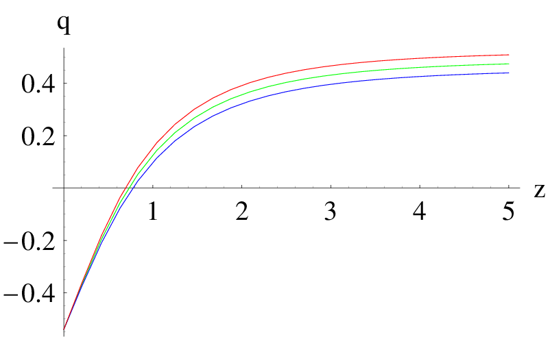
An intrinsic property of dark energy is that is does not interact with light. The only way that it may be observed is through its effect on the evolution of the background and its possible interaction with dark matter. In this section we look into how this model for quintessential dark energy affects the background by quantitatively looking at its effects on the rate of cosmic expansion and the fractional densities of dark matter and dark energy. A useful parameter used when considering cosmic acceleration is the “deceleration parameter”, . In an accelerating epoch, . In Fig. 8, we have shown a typical variation in the value of with redshift. The important feature of this reconstruction is that drops from positive to negative at , when cosmic acceleration began [90]. A nonzero coupling has an effect on the redshift when cosmic acceleration started, ; the positive coupling () implies an earlier start, and the negative coupling () implies a later start.

An alternative way of looking at the start of cosmic acceleration is to see when the effective equation of state drops below in Fig. 9. At high redshift, the effective equation of state goes towards , which is expected in the matter-dominated epoch (). For all values of , the effective equation of state goes to during the matter dominated epoch, but for large values of , . This is because the relative energy density of dark matter and dark energy now is fixed and the matter equation of state is constant, but the scalar equation of state is closer to for a larger , as shown in Fig. 5. At least, at low redshifts (), the effective equation of state does not vary much for different values of the coupling.


The relative energy density of dark matter to dark energy is affected by changes in the parameter, as seen in Fig. 10. For smaller values of , the matter density tends towards a lower value at high redshift. That is, due to the Friedmann constraint (33a), there is a higher proportion of dark energy during the matter dominated epoch for a small component. Here, it is clear that there has been an assumption made for the matter density today. The right hand side plot of Fig. 10 illustrates the effect of a non-minimal coupling on the evolution of matter density. The effect is not great within this small range, but there is a difference. A smaller value of the coupling parameter, , leads to an increase in the proportion of matter in the matter-dominated epoch. This study is valid for a range of low redshift, but will break down at high redshift when we enter the radiation-dominated epoch because we have made the assumption that the radiation component is negligible.


One requirement of the potential is that it should dominate the kinetic term so that the scalar field equation of state, , may be driven towards . It can be seen that this is satisfied by examining Figure 9. Recently, the authors of [62] have found two new diagnostic tools for distinguishing quintessential dark energy from Einstein’s cosmological constant. Their method may be extended to a non-minimally coupled theory for which . Here we simply note that for small values of and , satisfying the constraints given in table 2, the constraints of the present model encompass the cosmological constant limit at the level at low redshifts.
VII Conclusion
In this paper, a scalar-tensor theory of quintessential dark energy has been reconstructed. This reconstruction rests on the general action (6), in which the tensor theory of general relativity is modified by including a fundamental scalar field. The scalar field affects the gravitational part of the action by introducing a gravitationally repulsive term which drives the cosmic acceleration, and is coupled to the matter part of the action, giving rise to a nontrivial dark matter - dark energy interaction. As for all quintessence models, this action reduces to the one of general relativity, when the scalar field is time-independent and the coupling of dark matter to a scalar field (or dark energy) is minimal.
We made an ansatz for the form of the scalar field itself, in order to be able to reconstruct relevant cosmological parameters, including and . The ansatz for the scalar field was motivated by generic solutions of the dilaton field in some effective string theory models in four dimensions. The two new parameters, and as well as the matter scalar coupling parameter, , were constrained using several cosmological methods. Primarily, the relationship between and was constrained by curve-fitting to various cosmological data sets. For example, with and minimal coupling, using just the SN1a data, minimizing gave and using all the data sets available gave .
We also considered the effect of dark energy on the growth of large scale structure. The effect of a nonminimal coupling on the standard expression for the rate of growth of matter perturbations, , was considered. A modified ansatz for the dependence of matter density and dark matter-dark energy coupling on the matter fluctuation growth rate was introduced and then fitted to some observed values of the growth rate at low redshift. This analysis gave a best-fit minimum value for the coupling (with the input ), which is compatible with the minimally coupled scalar field case. These methods of constraining the variables of the model have succeeded in constraining , but failed in constraining the separate values of and . This is a direct result of taking the small limit when analyzing the solution for . Nevertheless, by assuming the same field for the inflaton as quintessence the individual values of and were constrained using the spectral index of the CMB. We find and .
Our analysis showed that the present model of coupled quintessence is compatible with a cosmological constant (where and ), within error bars. This means that dark energy may still simply be a cosmological constant, but even a small deviation away from this limit results in a very different source of cosmic acceleration, with time varying behavior. The number of parameters of this model may make it hard to rule out, as they may be tuned to satisfy many more constraints. In this work, the matter scalar coupling parameter was chosen to be a constant. This was not motivated physically but was chosen for the solvability of the system. Indeed, there is no physical reason why the dark energy - (dark) matter interaction should not vary in time, it is in all likelihood a function of . There needs to be further study to explore this dependence of . Also, the links between quintessential dark energy and inflation deserve further investigation.
References
- [1] A. G. Riess et al. (Supernova Search Team Collaboration), Astron. J. 116, 1009 (1998) [arXiv:astro-ph/9805201].
- [2] S. Perlmutter et al. (Supernova Cosmology Project Collaboration), Astrophys. J. 517, 565 (1999) [arXiv:astro-ph/9812133].
- [3] A.G. Riess et al. (Supernova Search Team Collaboration), Astrophys. J. 607, 665 (2004) [astro-ph/0402512].
- [4] R. A. Knop et al. Astroph. J. 598, 102(K) [arXiv:astro-ph/0309368].
- [5] http://lambda.gsfc.nasa.gov/
- [6] D. N. Spergel et al. [WMAP Collaboration], First Year Wilkinson Microwave Anisotropy Probe (WMAP) Observations: Determination of Cosmological Parameters, Astrophys. J. Suppl. 148, 175 (2003).
- [7] D. N. Spergel et al. [WMAP Collaboration], Wilkinson Microwave Anisotropy Probe (WMAP) three year results: implications for cosmology, Astrophys. J. Suppl. 170, 377 (2007) [arXiv:astro-ph/0603449].
- [8] S. M. Carroll, V. Duvvuri, M. Trodden and M. S. Turner, Is cosmic speed-up due to new gravitational physics?, Phys. Rev. D 70, 043528 (2004) [arXiv:astro-ph/0306438].
- [9] S. Capozziello, V. F. Cardone, S. Carloni and A. Troisi, Curvature quintessence matched with observational data, Int. J. Mod. Phys. D 12, 1969 (2003) [arXiv:astro-ph/0307018].
- [10] S. Nojiri and S. D. Odintsov, Modified gravity with negative and positive powers of the curvature: Unification of the inflation and of the cosmic acceleration, Phys. Rev. D 68, 123512 (2003) [arXiv:hep-th/0307288];
- [11] P. J. E. Peebles and B. Ratra, Cosmology with a time variable cosmological ‘constant’, Astrophys. J. 325, L17 (1988).
- [12] C. Wetterich, Cosmology and the Fate of Dilatation Symmetry, Nucl. Phys. B 302, 668 (1988).
- [13] I. Zlatev, L. M. Wang and P. J. Steinhardt, Quintessence, Cosmic Coincidence, and the Cosmological Constant, Phys. Rev. Lett. 82, 896 (1999) [arXiv:astro-ph/9807002].
- [14] E. Elizalde, S. Nojiri, S. D. Odintsov, D. Saez and V. Faraoni, Reconstructing the universe history, from inflation to acceleration, with phantom and canonical scalar fields, Phys. Rev. D 77, 106005 (2008) [arXiv:0803.1311 [hep-th]].
- [15] S. Nojiri, S. D. Odintsov and M. Sasaki, Gauss-Bonnet dark energy, Phys. Rev. D 71, 123509 (2005) [arXiv:hep-th/0504052].
- [16] B. M. N. Carter and I. P. Neupane, Dynamical relaxation of dark energy: Solution to both the inflation and the cosmological constant, Phys. Lett. B 638, 94 (2006) [arXiv:hep-th/0510109].
- [17] B. M. N. Carter and I. P. Neupane, Towards inflation and dark energy cosmologies from modified Gauss-Bonnet theory, JCAP 0606, 004 (2006) [arXiv:hep-th/0512262].
- [18] I. P. Neupane, Towards inflation and accelerating cosmologies in string-generated gravity models, arXiv:hep-th/0605265.
- [19] S. Tsujikawa and M. Sami, String-inspired cosmology: Late time transition from scaling matter era to dark energy universe caused by a Gauss-Bonnet coupling, JCAP 0701, 006 (2007) [arXiv:hep-th/0608178].
- [20] I. P. Neupane, On compatibility of string effective action with an accelerating universe, Class. Quant. Grav. 23, 7493 (2006) [arXiv:hep-th/0602097].
- [21] M. Li, A model of holographic dark energy, Phys. Lett. B 603, 1 (2004) [arXiv:hep-th/0403127].
- [22] H. Wei and R. G. Cai, A New Model of Agegraphic Dark Energy, Phys. Lett. B 660, 113 (2008) [arXiv:0708.0884].
- [23] I. P. Neupane, Remarks on Dynamical Dark Energy Measured by the Conformal Age of the Universe, Phys. Rev. D 76, 123006 (2007) [arXiv:0709.3096].
- [24] I. P. Neupane, A Note on Agegraphic Dark Energy, Phys. Lett. B 673 (2009) 111 [arXiv:0708.2910].
- [25] C. Deffayet, G. R. Dvali and G. Gabadadze, Accelerated universe from gravity leaking to extra dimensions, Phys. Rev. D 65, 044023 (2002) [arXiv:astro-ph/0105068].
- [26] P. K. Townsend and M. N. R. Wohlfarth, Accelerating cosmologies from compactification, Phys. Rev. Lett. 91, 061302 (2003) [arXiv:hep-th/0303097].
- [27] C. M. Chen, P. M. Ho, I. P. Neupane and J. E. Wang, A note on acceleration from product space compactification, JHEP 0307, 017 (2003) [arXiv:hep-th/0304177].
- [28] I. P. Neupane, Accelerating cosmologies from exponential potentials, Class. Quant. Grav. 21, 4383 (2004) [arXiv:hep-th/0311071].
- [29] N. Ohta, A study of accelerating cosmologies from superstring/M theories, Prog. Theor. Phys. 110 (2003) 269 [arXiv:hep-th/0304172].
- [30] I. P. Neupane, Simple cosmological de Sitter solutions on dS spaces, Class. Quan. Grav. 27 (2010) 045011 [arXiv:0901.2568];
- [31] I. P. Neupane, Accelerating universe from warped extra dimensions, Class. Quant. Grav. 26 (2009) 195008 [arXiv:0905.2774].
- [32] D. L. Wiltshire, Exact solution to the averaging problem in cosmology, Phys. Rev. Lett. 99 (2007) 251101 [arXiv:0709.0732].
- [33] D. L. Wiltshire, Dark energy without dark energy, arXiv:0712.3984 [astro-ph].
- [34] P. J. E. Peebles and B. Ratra, The cosmological constant and dark energy, Rev. Mod. Phys. 75 (2003) 559 [arXiv:astro-ph/0207347].
- [35] U. Alam, V. Sahni, T. D. Saini and A. A. Starobinsky, Is there Supernova Evidence for Dark Energy Metamorphosis?, Mon. Not. Roy. Astron. Soc. 354 (2004) 275 [arXiv:astro-ph/0311364].
- [36] V. Sahni, Dark matter and dark energy, Lect. Notes Phys. 653 (2004) 141 [arXiv:astro-ph/0403324].
- [37] E. J. Copeland, M. Sami and S. Tsujikawa, Dynamics of dark energy, Int. J. Mod. Phys. D 15 (2006) 1753 [arXiv:hep-th/0603057].
- [38] M. Sami, Dark energy and possible alternatives, arXiv:0901.0756 [hep-th].
- [39] Z. K. Guo, N. Ohta and Y. Z. Zhang, Parametrization of quintessence and its potential, Phys. Rev. D 72 (2005) 023504 [arXiv:astro-ph/0505253].
- [40] S. Weinberg, The cosmological constant problem, Rev. Mod. Phys. 61 (1989) 1.
- [41] V. Sahni, The cosmological constant problem and quintessence, Class. Quant. Grav. 19 (2002) 3435 [arXiv:astro-ph/0202076].
- [42] T. Padmanabhan, Cosmological constant: The weight of the vacuum, Phys. Rept. 380 (2003) 235 [arXiv:hep-th/0212290].
- [43] I. P. Neupane, Reconstructing a model of quintessential inflation, Class. Quant. Grav. 25 (2008) 125013 [arXiv:0706.2654].
- [44] E. Komatsu et al. [WMAP Collaboration], Five-Year Wilkinson Microwave Anisotropy Probe (WMAP) Observations:Cosmological Interpretation, arXiv:0803.0547 [astro-ph].
- [45] D. J. Eisenstein et al. [SDSS Collaboration], Detection of the Baryon Acoustic Peak in the Large-Scale Correlation Function of SDSS Luminous Red Galaxies, Astrophys. J. 633 (2005) 560 [arXiv:astro-ph/0501171].
- [46] A. G. Riess et al., New Hubble Space Telescope Discoveries of Type Ia Supernovae at : Narrowing Constraints on the Early Behavior of Dark Energy, Astrophys. J. 659 (2007) 98 [arXiv:astro-ph/0611572].
- [47] P. Astier et al. [The SNLS Collaboration], The Supernova Legacy Survey: Measurement of , and from the First Year Data Set, Astron. Astrophys. 447 (2006) 31 [arXiv:astro-ph/0510447].
- [48] C. Brans and R. H. Dicke, Mach’s principle and a relativistic theory of gravitation, Phys. Rev. 124 (1961) 925.
- [49] Y. M. Cho, Reinterpretation of Jordan-Brans-Dicke theory and Kaluza-Klein cosmology, Phys. Rev. Lett. 68 (1992) 3133.
- [50] Y. M. Cho and J. H. Kim, Dilatonic dark matter and its experimental detection, Phys. Rev. D 79 (2009) 023504 [arXiv:0711.2858].
- [51] G. Esposito-Farese and D. Polarski, Phys. Rev. D 63 (2001) 063504 [arXiv:gr-qc/0009034].
- [52] L. Amendola, Coupled quintessence, Phys. Rev. D 62 (2000) 043511 [arXiv:astro-ph/9908023].
- [53] T. Damour, G. W. Gibbons and C. Gundlach, Dark matter, time varying G, and a dilaton field, Phys. Rev. Lett. 64 (1990) 123.
- [54] T. Damour and G. Esposito-Farese, Tensor-scalar gravity and binary-pulsar experiments, Phys. Rev. D 54 (1996) 1474 [arXiv:gr-qc/9602056].
- [55] B. M. Leith and I. P. Neupane, Gauss-Bonnet cosmologies: crossing the phantom divide and the transition from matter dominance to dark energy, JCAP 0705 (2007) 019 [arXiv:hep-th/0702002].
- [56] I. P. Neupane, Constraints on Gauss-Bonnet Cosmologies, arXiv:0711.3234 [hep-th].
- [57] R. Bean, E. E. Flanagan, I. Laszlo and M. Trodden, Constraining interactions in cosmology’s dark sector, Phys. Rev. D 78 (2008) 123514 [arXiv:0808.1105].
- [58] M. B. Gavela, D. Hernandez, L. L. Honorez, O. Mena and S. Rigolin, Dark coupling, arXiv:0901.1611 [astro-ph].
- [59] I. P. Neupane and C. Scherer, Inflation and Quintessence: Theoretical Approach of Cosmological Reconstruction, JCAP 0805(2008) 009 [arXiv:0712.2468].
- [60] M. Chevallier and D. Polarski, Accelerating universes with scaling dark matter, Int. J. Mod. Phys. D 10 (2001) 213 [arXiv:gr-qc/0009008].
- [61] E. V. Linder, Exploring the expansion history of the universe, Phys. Rev. Lett. 90 (2003) 091301 (2003) [arXiv:astro-ph/0208512].
- [62] V. Sahni, A. Shafieloo and A. A. Starobinsky, Two new diagnostics of dark energy, Phys. Rev. D 78 (2008) 103502 [arXiv:0807.3548].
- [63] C. Cattoen and M. Visser, Cosmographic Hubble fits to the supernova data, Phys. Rev. D 78 (2008) 063501 [arXiv:0809.0537].
- [64] S. Weinberg, Gravitation and Cosmology, John Wiley and Sons, United State, 1972.
- [65] O. Lahav, P. B. Lilje, J. R. Primack and M. J. Rees, Dynamical effects of the cosmological constant, Mon. Not. Roy. Astron. Soc. 251 (1991) 128.
- [66] L. Guzzo et al., A test of the nature of cosmic acceleration using galaxy redshift distortions, Nature 451 (2008) 541 [arXiv:0802.1944].
- [67] L. Amendola, Linear and non-linear perturbations in dark energy models, Phys. Rev. D 69 (2004) 103524 [arXiv:astro-ph/0311175].
- [68] T. Damour and K. Nordtvedt, Tensor - scalar cosmological models and their relaxation toward general relativity, Phys. Rev. D 48 (1993) 3436.
- [69] B. Bertotti, L. Iess and P. Tortora, A test of general relativity using radio links with the Cassini spacecraft, Nature 425 (2003) 374.
- [70] T. Damour, F. Piazza and G. Veneziano, Runaway dilaton and equivalence principle violations, Phys. Rev. Lett. 89 (2002) 081601 [arXiv:gr-qc/0204094].
- [71] T. Chiba, T. Kobayashi, M. Yamaguchi and J. Yokoyama, Time variation of proton-electron mass ratio and fine structure constant with runaway dilaton, Phys. Rev. D 75 (2007) 043516 [arXiv:hep-ph/0610027].
- [72] S. Nesseris and L. Perivolaropoulos, The limits of extended quintessence, Phys. Rev. D 75 (2007) 023517 [arXiv:astro-ph/0611238].
- [73] S. Nesseris and L. Perivolaropoulos, Testing LCDM with the Growth Function: Current Constraints, Phys. Rev. D 77 (2008) 023504 [arXiv:0710.1092].
- [74] C. Di Porto and L. Amendola, Observational constraints on the linear fluctuation growth rate, Phys. Rev. D 77 (2008) 083508 [arXiv:0707.2686].
- [75] I. Antoniadis, J. Rizos and K. Tamvakis, Singularity - free cosmological solutions of the superstring effective action, Nucl. Phys. B 415 (1994) 497 [arXiv:hep-th/9305025].
- [76] M. Gasperini, F. Piazza and G. Veneziano, Quintessence as a runaway dilaton, Phys. Rev. D 65 (2002) 023508 [arXiv:gr-qc/0108016].
- [77] T. Barreiro, B. de Carlos and E. J. Copeland, Stabilizing the Dilaton in Superstring Cosmology, Phys. Rev. D 58 (1998) 083513 [arXiv:hep-th/9805005].
- [78] B. Boisseau, G. Esposito-Farese, D. Polarski and A. A. Starobinsky, Reconstruction of a scalar-tensor theory of gravity in an accelerating universe, Phys. Rev. Lett. 85 (2000) 2236 [arXiv:gr-qc/0001066].
- [79] C. Armendariz-Picon, V. F. Mukhanov and P. J. Steinhardt, Essentials of k-essence, Phys. Rev. D 63 (2001) 103510 [arXiv:astro-ph/0006373].
- [80] V. Sahni and A. Starobinsky, Reconstructing Dark Energy, Int. J. Mod. Phys. D 15 (2006) 2105 [arXiv:astro-ph/0610026].
- [81] R. J. Scherrer and A. A. Sen, Thawing quintessence with a nearly flat potential, Phys. Rev. D 77 (2008) 083515 [arXiv:0712.3450].
- [82] R. J. Scherrer and A. A. Sen, Phantom Dark Energy Models with a Nearly Flat Potential, Phys. Rev. D 78 (2008) 067303 [arXiv:0808.1880].
- [83] S. Dutta and R. J. Scherrer, Hilltop Quintessence, Phys. Rev. D 78 (2008) 123525 [arXiv:0809.4441].
- [84] N. J. Nunes, D. F. Mota Structure Formation in Inhomogeneous Dark Energy Models, Mon. Not. Roy. Astron. Soc. 368 (2006) 751 [astro-ph/0409481].
- [85] L. Samushia and B. Ratra, Constraints on Dark Energy from Galaxy Cluster Gas Mass Fraction versus Redshift data, Astrophys. J. 680 (2008) L1 [arXiv:0803.3775].
- [86] A. J. Albrecht and C. Skordis, Phenomenology of a realistic accelerating universe using only Planck-scale physics, Phys. Rev. Lett. 84 (2000) 2076 [arXiv:astro-ph/9908085].
- [87] H. Wei, Growth Index of DGP Model and Current Growth Rate Data, Phys. Lett. B 664 (2008) 1 [arXiv:0802.4122].
- [88] H. Wei and S. N. Zhang, How to Distinguish Dark Energy and Modified Gravity?, Phys. Rev. D 78 (2008) 023011 [arXiv:0803.3292].
- [89] U. Alam, V. Sahni and A. A. Starobinsky, Reconstructing Cosmological Matter Perturbations using Standard Candles and Rulers, Astrophys. J. 704 (2009) 1086 [arXiv:0812.2846].
- [90] A. Melchiorri, L. Pagano and S. Pandolfi, When Did Cosmic Acceleration Start?, Phys. Rev. D 76 (2007) 041301 [arXiv:0706.1314].