Using the Eigenvalue Relaxation for Binary Least-Squares Estimation Problems
Abstract
The goal of this paper is to survey the properties of the eigenvalue relaxation for least squares binary problems. This relaxation is a convex program which is obtained as the Lagrangian dual of the original problem with an implicit compact constraint and as such, is a convex problem with polynomial time complexity. Moreover, as a main pratical advantage of this relaxation over the standard Semi-Definite Programming approach, several efficient bundle methods are available for this problem allowing to address problems of very large dimension. The necessary tools from convex analysis are recalled and shown at work for handling the problem of exactness of this relaxation. Two applications are described. The first one is the problem of binary image reconstruction and the second is the problem of multiuser detection in CDMA systems.
1 Introduction
Several problems in engineering and in particular signal and image processing necessitate to estimate binary vectors corrupted by some noise and can be simply addressed using the least squares principle under binarity consraints. The resulting problem is a minimization of a quadratic form over , a problem which is known to be -Hard in general. One of the main approaches to relax this problem into a convex one is the Semi-Definite Programming relaxation which has been extensively used in classification, pattern recognition and communication systems. Some of the main achievements in the study of the SDP relaxation were obtained by Goemans and Williamson [13] and [11]. However, solving a SemiDefinite Program in practice relies on interior point methods which although enjoying nice theoretical convergence properties are limited to problems of size up to 500 . On the other hand, very pratically efficient bundle methods are available for the eigenvalue relaxation of the same binary quadratic optimization problems. We refer the reader to [1] for a discussion of the pratical superiority of bundle methods for solving certain semi-definite programs such as the ones appearing in the present paper. Despite this empirical fact in favor of the eigenvalue relaxation, one of the main reasons most users prefer the SDP relaxation is that good primal binary solutions can be recovered using Goemans and Williamson’s randomized algorithm. The main motivation of the present paper is to show how a solution of the SDP can be recovered from a solution of the eigenvalue relaxation. As a by product, a new geometric interpretation of the randomized algorithm is proposed.
Penalized binary least squares estimation problems are problems of the form
| (1.0.1) |
where the vector is the observed data, the matrix represents the ”filter”, the vector is the signal, or parameter vector, that has to be estimated, and the term is a penalization term that can often be interpreted as an a priori information in terms of Bayesian statistics.
This problem belongs to the larger class of minimization of quadratic forms over binary vectors which is known to be -hard. Much work has been devoted to constructing Semi Definite Programming (SDP) based relaxations for general quadratic binary problems. Semi-Definite programs are linear optimization problems over symmetric matrices with real coefficients and with the additional convex constraint of positive semidefiniteness; see for instance [6] or [2] for excellent introductions to convex programming and in particular SDP. SDP methods have already played an important role in various topics inside signal processing problems and we refer to [3] for a nice survey on possible applications. A common feature of essentially all the existing relaxations is that they can be obtained using Lagrange duality which is a general methodology for obtaining lower bounds to hard minimization problems, as overviewed in [4] and [5].
The goal of the paper is to survey what is known about another Lagrangian duality based relaxation, namely the eigenvalue relaxation, for this problem. This relaxation was first proposed by Delorme and Poljak [19] for the max-cut problem. See also the work of Poljak, Rendl and Wolkowics [7] for more details. The main advantage of the eigenvalue relaxation over the SDP relaxation is that the eigenvalue relaxation can be solved much faster than the SDP relaxation, as reported for instance in [1], [8], [9] and [10]. This remarkable computational tractability of the eigenvalue relaxation is the main motivation for writing this detailed survey.
The content of the paper is as follows. The second section is devoted to a rapid presentation of the relaxation and its relationship with Lagrangian duality. We also recall a simple and well known certificate for exactness of the relaxation, i.e. the fact that a globally optimal binary solution is obtained.
The third section details the relationships between the Semi-Definite Relaxation and the eigenvalue relaxation. The main result of this section is the following: a solution of the SDP relaxation can be recovered from the solution of the eigenvalue relaxation. The case of inexact solutions to the eigenvalue relaxation is also studied.
The forth section deals with the problem of recovering binary primal solutions from the dual scheme. We first give sufficient conditions under which strong duality holds and the eigenvectors of norm associated to the maximum eigenvalue at optimality are binary solutions. Next, in the case where strong duality does not hold, we show that Goemans and Williamson’s randomized algorithm has a very natural meaning when viewed in terms of the optimal eigenspace associated to the maximal eigenvalue in the eigenvalue relaxation.
In the last section, we propose simulation experiments in the case of binary image denoising and CDMA Multiuser Detection problems. The first of these problems has been previously approached by stochastic methods based on Markov chains like simulated annealing and Metropolis Hastings schemes; see for instance [17] and the more recent work of Gibbs [14]. The approach discussed here was presented in [15]. Recently a lot more problems have been addressed using the SDP relaxation in [16]. The results obtained so far are quite encouraging and the approach performs well on very dirty images. We prove hat strong duality holds for the immage denoising problem, thus recovering back the polynomial solvability result of Greig, Porteous and Seheult as a special case and by a very different path. Passing to the second problem, our Monte Carlo experiments show that the average computational effort for solving the eigenvalue relaxation as a function of the number of users grows slowlier than for the SDP relaxation with the standard implementations available with scilab.
Notations. In the sequel we will use the following notations. The inner product on is denoted by , the set of real symmetric matrices of order are denoted by . The partial order denotes the Loewner ordering, i.e. for and in , means that is positive semidefinite. For a set in , denotes the convex hull of and denotes its closure. For a matrix in , denotes its diagonal vector and for in , denotes the diagonal matrix whose diagonal vector is . If an equation number corresponds to an optimization problem, then will denote the optimum value for this problem.
2 The eigenvalue relaxation
We first introduce the eigenvalue relaxation and at the same time, we propose a quick refresher on Lagrangian duality, collecting all the results that will play an essential role in the sequel. The proofs of almost all the results presented here can be found in [18].
2.1 The Lagrangian dual and the eigenvalue relaxation
The binary least-squares estimation problem is in fact equivalent to the homogenized problem
Indeed, if we add the constraint in (BLS), we obtain exactly the binary least squares problem. Now, if is a solution of (BLS), then is again a solution of of (BLS), thus adding the constraint is in fact redundant, which proves the claimed equivalence. Set
Notice further that the constraint is equivalent to for all . Thus, to problem (BLS), we can associate the Lagrangian function
Now we can add to the problem the implicit spherical constraint
which is redundant with the binary constraints. Then, optimizing over this sphere, we obtain the Lagrangian dual function, i.e.
which, using Raleigh-Ritz variational formulation of the largest eigenvalue of symmetric matrices, can be written
| (2.1.1) |
Finally, the dual problem, i.e. the eigenvalue relaxation, is given by
| (2.1.2) |
2.2 Properties of the dual relaxation
2.2.1 Convexity
It is important to notice first that the dual function is convex, since it is the maximum over a family parametrized by of linear functions in the variable .
2.2.2 Weak duality
The main classical property of the Lagrangian dual is weak duality, i.e.
where denotes the optimal value.
This property explains in part why Lagrange duality is used : it provides a bound on the primal optimal value. When equality holds in the weak duality property, we say that strong duality holds. Sometimes, like in the case of the Max-Cut problem, the bound can be proved to be proportional to the optimal original value. More precisely, Goemans and Williamson proved that the optimum value of the eigenvalue relaxation (in fact the equivalent SDP formulation; see the original paper and Section 3 below) is greater than or equal to the optimal original value (this is just weak duality), which itself is always greater than or equal to .876 times the eigenvalue relaxation’s optimal value. A quite similar but less tight bound, proved by Nesterov applies directly to the present problem. We will recall this bound in section 4.2.1 below.
2.2.3 Existence of dual solutions
It is well known that there exists an optimal dual solution. This was proved by Poljak and Wolkowicz in [20]. The proof given here is more direct.
Proposition 2.2.1
The dual function admits a minimizer.
Proof. Let . Make the change of variable , i.e. define
We now have the property that . We prove that is coercive. Take any sequence with as . We can assume that for some because otherwise, the fact that implies that there must exists a sequence with and the fact that gives a contradiction. Now, the Gershgorin circle around the diagonal element has a constant radius, say and its center goes to . Since , this implies that . Thus is coercive and since it is continuous, it admits a minimizer that we will denote by . Now, for all , , we have
But, on the other hand, . Therefore,
and the proof is complete.
2.2.4 Subdifferential’s description and exactness criterion
The subdifferential of the eigenvalue relaxation has been much studied. Recall that for any convex function , the subdifferential is defined by
The analysis of is based on the following general theorem.
Theorem 2.2.2
[18] Let be an affine operator defined by for some linear operator and some matrix . Then, we have
with
where is the adjoint of , denotes the multiplicity of at and is a matrix whose columns form any orthonormal basis of the eigenspace of associated to .
Now, if we set , we get , and . For , let be defined by
Using the previous theorem, we obtain
Corollary 2.2.3
The subdifferential of the dual function is given by
Following Oustry [8], the formula for in theorem 2.2.2 is proved by showing that the maximum eigenvalue function on is nothing but the support function of , defined by
with the scalar product defined by . By definition, the face of exposed by is the set of maximizers in (2.2.4), i.e.
Knowing that the subdifferential of a support function of a set is exactly the exposed face of this set, we finally get
the formula follows after some linear algebra.
There is a different path to the subdifferential’s formula, which is perhaps more a propos in the context of duality: it is proved in [18, Chapter XII] that
| (2.2.1) |
where denotes the closure of the convex hull. This fact is in fact true for general continuous constrained problems in the case where the underlying space is compact (for example) 11 1 which is the case here since we optimize over the sphere and the associated technical condition is called the filling property. The following proposition provides a useful sufficient condition for proving that the relaxation is exact, i.e. strong duality applies.
Proposition 2.2.4
Let be a minimizer of the dual eigenvalue relaxation. Then, if has multiplicity one, then
and any eigenvector of whose squared norm is is a binary solution of (BLS).
The proof is a direct consequence of [18, Theorem XII.2.3.4.]. We provide a specialized proof here because it is short and instructive.
Proof. Since the multiplicity of is one, the subdifferential of at is a single vector. Thus, is differentiable at and its gradient is simply
for any in such that . Since, minimizes , we must have . This implies that for all . Thus, using weak duality
which proves that solves the original problem (BLS).
We now have a nice criterion for deciding whether our relaxation was exact and if so, we also know how to recover a binary solution from an optimal eigenvector. This approach works for any quadratic binary problem and is extensively used for approximating combinatorial problems. However, the question remains on what to do when the relaxation is not exact, i.e. when the multiplicity at the optimum is greater than one. The next two sections will help answer this crucial question.
3 From eigenvectors to SDP solutions
The purpose of the next two sections is to describe how to recover primal binary solutions from the eigenvector solutions of the dual eigenvalue problem. It was first shown that good binary solution can be generated at random using the SDP solution by Goemans and Williamson [13] in the case of the Max-Cut problem in graph theory. Their results were then extended by Nesterov to the case of indefinite quadratic binary programming [11]. Those results allowed to conclude that both eigenvalue and SDP relaxations are in a certain precise sense very efficient. However, both relaxations are not equivalent from the computational point of view. Recall that one of the main motivations for using the eigenvalue relaxation is its manageable practical complexity which is often favorable compared to the one of solving the SDP relaxation. But what is not clear is how to generate good (primal) binary solutions in average with the eigenvalue relaxation only ? The first natural approach to this question is of course to try and recover an optimal SDP solution from the eigenvalue relaxation. Thus, we devote this section to this problem. It can be solved as follows : an appropriate convex combination of rank one matrices obtained from a set of optimal eigenvectors is shown to be a solution we are looking for. Our approach simplifies the presentation of [21]. The adaptation of the randomized algorithm of Goemans and Williamson and the associated bound established by Nesterov will be discussed in the next section.
3.1 The SDP relaxation
In order to obtain the Semi-Definite Programming (SDP) relaxation of the the homogenized problem (BLS), we begin with the following equivalence relating our problem to a problem on symmetric matrices. We have 22 2 Here, we use the fact that
This last problem is itself equivalent to
This problem being nonconvex, we drop the rank constraint and obtain the following SDP (convex) relaxation
whose value is obviously greater than or equal to .
An important result of Pataki [36, Theorem 2.1] gives a bound on the rank of solutions to Semi-Definite Programs. In the case of our Semi-Definite relaxation, this theorem implies that the rank of an optimal matrix satisfies .
3.2 SDP versus maximal eigenvalue : theoretical equivalence
It follows from the subdifferential’s formula given in Corollary 2.2.3 that at any minimizer , we have
Suppose we have in hand a matrix such that
| (3.2.1) |
It appears that a good guess for a candidate solution to the SDP relaxation in the general case is
We just need to check the details to see how it works. This result was initially proved in [21] but the proof given here is more direct.
Theorem 3.2.1
Remark 3.2.2
We would like to underline at this point that a more elegant proof of the theorem could be obtained using conic duality but we preferred to keep on with elementary arguments since this is possible in the present context.
Proof. Compute the eigenvalue/eigenvector decomposition , set , , let be the multiplicity of and let denote the columns of . Recall that from the definition of , we have . Then, we get
Thus,
Using this fact, we obtain
since . Thus, the optimal value of the SDP is greater than or equal to the optimal value of the eigenvalue relaxation. On the other hand, it is well known that the optimal value of the eigenvalue relaxation is greater than or equal to the one of the SDP relaxation. We provide a proof here for the sake of completeness. Let be an optimal solution to the SDP relaxation. Now, for all in , we have
by using the fact that . Now, compute the eigenvalue/eigenvector decomposition and let be the greatest of these eigenvalues. Then,
Since this is true for all , we obtain that the eigenvalue relaxation majorates the SDP relaxation. Thus, both optimal values are equal and this completes the proof of the proposition.
3.3 SDP versus maximal eigenvalue: practical implementation
Of course, it can be hard to find a matrix that works. We will now try to overcome this problem. We first have to specify how the subgradients are obtained in practice. At each point , choose an eigenvector of squared norm equal to associated to . Then, using the alternative representation of the subdifferential (2.2.1), a subgradient of at is obtained by setting . Assume that we have a set of subgradients for some , and such that
for some nonnegative ’s with . This can be performed for as small as we want by using a bundle method. Such a method will construct in a finite number of iterations, say , an iterate and a family of ’s with the desired property, all of them lying in a small neighborhood of . This is one very nice feature of the bundle mechanism which is extensively described in [18, Volume II]. Moreover, it is a well known fact, called Caratheodory’s theorem, that only subgradients are sufficient in the expression (OPT).
Set
Then, we have the following result.
Proposition 3.3.1
For any , the matrix defined above satisfies
Proof. Let be any minimizer of . Then, for each , we have by the definition of the subdifferential
But is given by
On the other hand, since ,
Thus, we obtain
which implies, after multiplying by and summing over
Using Cauchy-Schwartz inequality, this gives
Since the eigenvalue and the SDP relaxation have equal optimal values, we finally obtain
which implies the desired result.
3.4 Comments
It is a common idea that the SDP relaxation contains more information than the eigenvalue relaxation. We hope that the results of this section managed to convince the reader that this is in fact not the case and a good approximate solution can be recovered quite easily using subgradient information at the optimum.
4 Recovering primal binary solutions
We now are in position to answer our main question of how to recover a satisfactory although sometimes suboptimal primal binary solution. In the first part of this section, we show that optimal binary solutions can actually be exactly recovered using the eigenvalue relaxation, i.e. strong duality holds, under some simple conditions. Then, in the case where the problem does not satisfy these necessary conditions for strong duality, we develop a randomized algorithm based on the optimal eigenspace of the maximum eigenvalue dual function and show that this procedure is equivalent to Goemans and Williamson’s randomized algorithm for Max-Cut. This provides a new interpretation of Goemans and Williamson’s procedure.
4.1 A sufficient conditions for strong duality
We have the following theorem.
Theorem 4.1.1
For almost all in the sense of the Lebesgue measure, such that is componentwise negative outside the diagonal. Then the eigenvalue relaxation is exact, i.e. strong duality holds.
Proof. Fix . Let be the vector of the first components of . The fact that is componentwise negative outside the diagonal implies that is componentwise positive. Thus, the Perron-Frobenius theorem implies that the maximum eigenvalue of has multiplicity one. From this, we deduce that the maximum eigenvalue of also has multiplicity one. Let be an eigenvalue decomposition of , where we used the subscript in order to remember that whatever the chosen decomposition, it is a nonlinear and non necessarily continuous function of . Moreover, since the maximum eigenvalue has multiplicity one, Corollary 4 in [22] says that it is possible to choose the eigenvector associated to the maximum eigenvalue as a continuously differentiable function of . We will denote by this eigenvector. Using this parametrization, the matrix
can be rewritten as
where all dimensions can easily be guessed from the previous knowledge on the involved submatrices.
Let be the codimension one differentiable submanifold defined by
Let be the optimal set defined by
Due to the representation
the set is the projection onto the cartesian product of the set where is the upper bound of Pataki (see Section 3.1) on the optimal rank of the SDP relaxation33 3 which also holds for the eigenvalue relaxation due to the complete equivalence between these two problems (here for large) and where is the set
whose intersection with corresponds to the parameter set allowing for zero to belong to the subdifferential of the dual function in the case where . Now, since the constraint is described by equations, by equations, by one equation and , the dimension of is greater than or equal to . Furthermore, notice that since the eigenvalues are continuous fonctions of the entries of , the subset of for which is open in the topology induced by the ambiant space. Therefore its projection set onto the cartesian product is of dimension at least which garantees that the projection onto the -space of its intersection with is a set of null Lebesgue measure. And thus, for almost all , such that is componentwise negative outside the diagonal, .
Using this result, Theorem A about the interlacing property of the eigenvalues for arrow matrices in the Appendix implies that the maximum eigenvalue of is greater than the maximum diagonal element of which nothing by and all other eigenvalues are less than . This implies that for allmost all , the maximum eigenvalue of has multiplicity one at the optimum, which implies that is differentiable at the optimum. Therefore, using Proposition 2.2.4 we obtain that strong duality holds for allmost all such that is componentwise negative outside the diagonal.
4.2 When strong duality fails: the randomized algorithm
We start this section with some recalls on Goemans and Williamson’s algorithm and Nesterov’s bound.
4.2.1 Goemans and Williamson’s algorithm and Nesterov’s bound
The method relies on the Cholesky factorization of the optimal solution of the SDP relaxation,
From Theorem 3.2.1 we see that where is the multiplicity of at the chosen corresponding solution of the eigenvalue relaxation. This factorization is important, since it allows to write where is the transpose of row vector of . Let be a random variable with uniform distribution on the unit sphere in .
Procedure 4.2.1
(Goemans and Williamson’s algorithm)
1. Find the Cholesky factorization .
Let be a random vector with uniform distribution on the unit sphere of . The random cut is defined by
where the sign function is defined coordinate-wise.
2. Draw samples from , say , …, and choose the sample giving the best value of the objective function .
The key result is that, in average, the vector gives a good binary solution to the original problem. Since the best sample will have greater cut value than the average with overwhelming probability, the above procedure should work well. This is made precise by Nesterov’s theorem.
Theorem 4.2.2 (Nesterov)
Define
and
then, we have
This result is remarkable despite the fact that the bound is rather large. An important issue for future research is to study such type of bounds for particular subclasses of problems in hope of improving Nesterov’s result.
4.2.2 The eigenvector viewpoint
The main drawback of the former presentation is that using the uniform variable is quite hard to motivate from an optimization viewpoint. Let us take a slightly different perspective. Assume that we have a solution of the eigenvalue relaxation. As before, let be a matrix whose columns form an orthonormal bases of the eigenspace associated to . Moreover, we may require that
| (4.2.1) |
where is some diagonal matrix with , and . In the case where the multiplicity at the optimum is one, the optimal eigenbasis reduces to a unique vector and we saw in Proposition 2.2.4 that multiplying this vector by gives a binary solution. Now let us turn to the case where there are eigenvectors. To each unit norm eigenvector , we associate a subgradient . Then, (4.2.1) implies that
-1,-1)(2,2)
Now one natural strategy might be the following: pick the best eigenvector, i.e. the eigenvector whose associated coefficient in expression (4.2.2) is the greatest and round its coordinates to the nearest binary values. There is a second strategy : draw random linear combinations of the ’s giving preference to the components with higher associated coefficient in (4.2.2). This can be done by sampling vectors of the type
where the ’s are independent random variables with distribution . For each sample, a feasible solution is obtained by rounding off the components to the nearest binary. We sum up this procedure as follows.
Procedure 4.2.3
(Randomized algorithm based on optimal eigenvectors) 1. Find the matrix whose columns form an orthonormal eigenbasis associated to such that (4.2.2) holds for some ’s satisfying and .
2. Let be a random vector with distribution . The random cut is defined by
3. Draw samples from , say , …, and choose the sample giving the best value of the objective function .
The important result is that this second strategy is equivalent to Goemans and Williamson’s randomized procedure.
Proposition 4.2.4
Procedure 4.2.3 is equivalent to Goemans and Williamson’s algorithm.
Proof. Set . Then Theorem 3.2.1 and equation 4.2.2 imply that with , thus retrieving the Cholesky factorization of . Let . It is clear that has distribution . This proves that the cut obtained by Procedure 4.2.3 is exactly the output of Goemans and Williamson’s procedure.
The eigenvalue point of view thus allowed us to provide an alternative and geometric explanation for taking a random cut using a uniformly distributed variable on the sphere in Goemans and Williamson’s methodology.
5 Two application examples
In this section, we provide some results for the concrete problems of image denoising and show how this relaxation applies to the problem of multiuser detection in CDMA systems.
5.1 Image denoising
5.1.1 Presentation of the problem
The first set of simulations is devoted to the denoising problem, in which is simply the identity matrix. This is the problem considered in [23], [14] and [17] for instance. The original binary image as 26 rows and 62 columns which gives a total number of 1612 variables.
For this problem, the penalization matrix is chosen so as to smooth the image. This is achieved by requiring neighboring pixels to be similar in the sense that if and are indices of neighbor pixels, then, we would like the least square cost to be penalized by the quantity . Thus, is the matrix associated to the quadratic form
| (5.1.1) |
where denotes the property of being neighbor indices and the are nonnegative. The neighborhood of each pixel is usually chosen to be the north, south, east and west pixels.
5.1.2 Exactness of the relaxation
The following theorem is the main result of this section.
Theorem 5.1.1
For , the identity matrix and the matrix associated to the quadratic form (5.1.1), the eigenvalue relaxation is exact.
Proof. The eigenvalue relaxation of the optimization problem corresponding to this binary least square denoising problem is as before
Consider now the perturbed optimization problem
where is negative outside the diagonal. Since the are nonnegative, the matrix has only nonpositive off diagonal terms and thus, Theorem 4.1.1 proves that strong duality holds for this problem and there exists a binary eigenvector that achieves optimality. Assume that is chosen so that . Then, the optimum value of problem (Denoise) and the optimum value of problem (Perturbed) satisfy
Moreover, by weak duality, we have
Since strong duality holds for problem (Perturbed), denoting by a solution of we have
Therefore, we obtain
which implies
Now, since is finite, the image of by the function is a finite set. Let denote the closest number to in . Now, choosing , we obtain
which proves that the denoising problem is polynomial time solvable by solving problem (Perturbed).
This theorem is to be compared with the results of D. M. Greig, B. T. Porteous and A. H. Seheult [34] which formulates the binary denoising problem as a minimization problem with cost given at the top of page 273. The objective to be minimized in [34] can be rearranged so as to minimize a linear cost with same penalization as the one given by (5.1.1). The main contribution of [34] is to say that this problem can be solved in polynomial time using a network flow algorithm. Notice that our proof works for and any additional linear term added to the penalized objective function to be optimized. Since the eigenvalue relaxation can also be optimized in polynomial time, this confirms that the eigenvalue relaxation performs at least as good as previous approaches on a well known problem. On the other hand, the eigenvalue relaxation can be a flexible approach in more complicated cases where is not equal to the identify or other quadratic constraints have to be incorporated such as in [16].
5.1.3 A numerical experiment
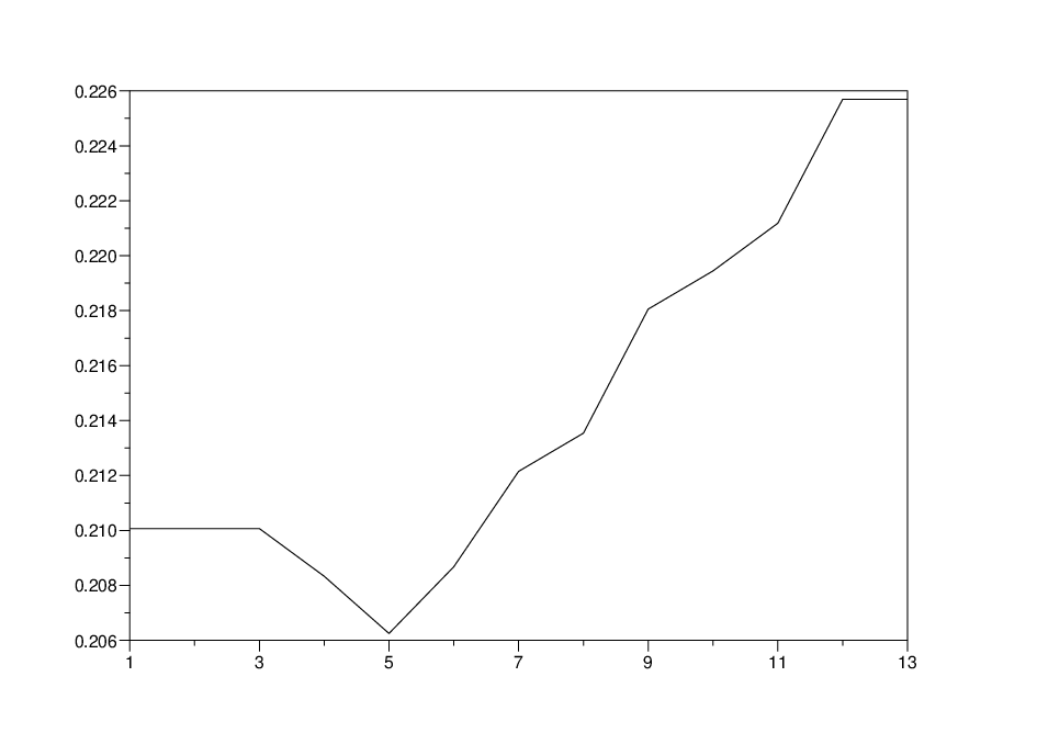
The experiments reported on below were performed for the case of quite noisy original images. The noise was taken to be additive, independent identically distributed and Gaussian and was applied to the symmetrized image with pixel values in . In order to show the influence of the smoothing parameter , we displayed the percentage of misspecified bits vs values of . The recovered image is the one with the choice of giving the best percentage of bits recovered.
We found the results very encouraging. Indeed, even when the observed image is very noisy, we still recover an image which is readable. This suggested that an appropriate postprocessing might easily allow to recover the original written words, by comparing the letters to a given dictionary. Cross validation can be used to estimate . We will not discuss this problem here. Instead, it seems reasonable to argue that the choice of can just be made a posteriori since it consists of tuning the method until a satisfactory solution is obtained. This reduces the hard combinatorial initial problem to a simpler one parameter knobing procedure. The displayed experiment and the numerous simulations not presented here confirm that robust intervals for the values of are not very difficult to identify in practice.
5.2 Multiuser detection in CDMA systems
5.2.1 Presentation of the problem
This problem was studied by [24] using the maximum likelihood approach. As we will see, the resulting optimization problem is of the same form as the binary least squares problem. The main difference here is that and .
A synchronous K users DS-CDMA system is considered with a common single path additive white Gaussian noise (AWGN) channel. The signature waveform of the th user is denoted by , a function taking nonzero values in and being equal to zero outside this interval, and is the information bit transmitted by user . The overall received signal is therefore of the form
where is the amplitude of the th user’s signal and is an additive white Gaussian white noise with zero mean and variance . The signal is then filtered using a bank of matched filters. The output of the th matched filter is given by
In matrix form, this can be written
where , is the correlation matrix whose components are given by , and is the vector with components .
Since the gaussian vector has a correlation matrix equal to , the ML estimator is obtained by simply solving the following combinatorial optimization problem.
| (5.2.1) |
5.2.2 Some comments
The SDP approach seems to have been first applied for the DS-CDMA detection problem in [26]. Since then numerous contributions have appeared using the SDR and comparing it to other methods as in [28] and [29]. Extension to M-ary phase shift keying symbol constellations is proposed in [30]. The issue of accelerating the speed of the method is addressed in [31]. However, as for the former problem, the main drawback of the standard primal semidefinite relaxation is that the size of the problem is greatly increased by using matrices instead of vectors of size . In order to overcome this problem, a better approach using semidefinite programming duality was recently proposed in [32].
The analysis of the previous sections proves that the eigenvalue relaxation is equally applicable to this problem and maybe a good competitor to the SDP relaxation. The most important point of our analysis is the following: Theorem 4.1.1 proves that if the correlation matrix is componentwise negative outside the diagonal, then strong duality holds, i.e. the detection problem can be solved exactly in polynomial time. The construction of efficient signatures is the current subject of an active research activity. For instance, the theory of frames allows to consider the problem from an interesting viewpoint as developed in [35]. Our findings suggest in particular that the componentwise negativity of the correlation matrix may be an interesting constraint to look at in future investigations on this problem.
-1,-1)(1,1)
-¿(0,0)(0,1) 0).5-3090
Finally, the eigenvalue relaxation can also be useful even for general signatures because of the weak duality property. Indeed, several recent publications prove that clever heuristics can perform better than the SDP relaxation. However, in real situations it is hard to certify that a primal solution provided by such a heuristic is indeed the optimal solution because the original signal is unknown. Comparing the dual optimal value to a primal value given by a heuristic can give a precise idea of the error without prior information on the signal.
5.2.3 A numerical experiment
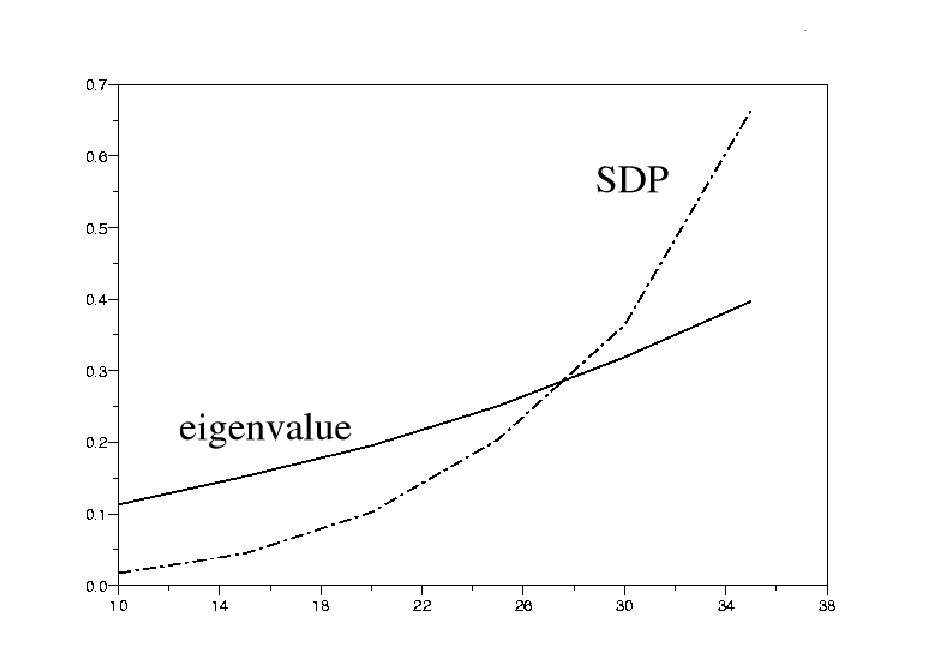
In order to verify this point, we performed Monte Carlo simulations over 1000 random problems for a number a users varying from 10 to 35. These computational experiments are reported in Figure 7 where the number of users is on the x-axis and the average computation time is on the y-axis. The computations where performed using the Scilab software [33]. The SDP solver called Semidef interfaces Boyd and Vandenberghe’s sp.c program. The eigenvalue relaxation was solved using the solver Optim with the ”nd” option for possibly nondifferentiable costs as is the case here. The curves in Figure 7 interpolate the average computation times for messages taken to be sequences of uniform and independant variables taking values in vs. the number of users. The curve with dashed style is for the results of the SDP relaxation while the curve with plain style is for the eigenvalue relaxation. Our computations suggest that the eigenvalue relaxation has lower complexity growth as the number of users increases exactly as expected. The reader should be warned that this experiment does not prove that the complexity of the eigenvalue relaxation is lower than the SDP relaxation. The experiment only shows that when a widely used routine for SDP is used, the eigenvalue relaxation, solved using a general purpose bundle method available through a free a well established software, has a lower complexity growth on this problem.
6 Appendix: Arrow matrices and strict interlacing of eigenvalues
Arrow matrices are matrices of the form
The properties of the eigenvalues of such matrices have been well studied in the past. Some of them are summarized in the following theorem. Theorem A. Let be an arrow matrix, with . Moreover, assume that all the components of are different from zero. Let be its eigenvalues considered in increasing order. Then, the characteristic polynomial of is given by
Then, we have and . Moreover,if we have and if , we have .
The properties of the eigenvalues of arrow matrices are part of the folkore, especially in the realm of mathematical physics. We give a sketch of the proof of this theorm below in order to give the main ideas underlying the results.
Proof of Theorem A. The formula for the characteristic polynomial is easily obtained by reccurence on the dimension. We have to consider two cases:
- •
for some , ,
- •
In the first case is a root of . In the second case which is different from zero since we assumed all the ’s to be different from zero. In this case, the eigenvalues of are the zeros of the function
From this formula, we deduce that there is a root in each interval , , for all and .
The final conclusions are easily derived by combining the results in the two simple cases discussed above.
7 Conclusion
In this paper, we surveyed the main properties of the eigenvalue relaxation for binary least squares problem. A full connection with the standard SDP relaxation was presented and we showed how to recover a solution of the Semi-Definite program from the solution of the eigenvalue minimization problem. The problem of recovering primal binary solution was also addressed and we gave simple sufficient conditions for strong duality. In the case where these conditions are not satisfied, the randomized procedure adapted from Goemans and Williamson’s allows to recover binary solutions with garanteed relative approximation ratio due to Nesterov’s bound. Two applications were presented: binary image denoising and detection in multiuser CDMA systems. In the case of image denoising, we show that strong duality holds. For the multiuser detection problem, our results prove that strong duality holds when the signature covariance matrix has nonpositive off diagonal components.
References
- [1] Lemaréchal C. and Oustry F., Nonsmooth algorithms to solve semidefinite programs, Recent Advances on LMI methods in Control, L. EL Ghaoui and S-I. Niculescu editors, SIAM (1999).
- [2] Boyd, Stephen and Vandenberghe, Lieven Convex optimization. Cambridge University Press, Cambridge, 2004
- [3] Luo, Zhi-Quan, Applications of convex optimization in signal processing and digital communication. ISMP, 2003 (Copenhagen). Math. Program. 97 (2003), no. 1-2, Ser. B, 177–207.
- [4] Lemaréchal, Claude and Oustry, François SDP relaxations in combinatorial optimization from a Lagrangian viewpoint. Advances in convex analysis and global optimization (Pythagorion, 2000), 119–134, Nonconvex Optim. Appl., 54, Kluwer Acad. Publ., Dordrecht, 2001.
- [5] Wolkowicz, Henry and Anjos, Miguel F. Semidefinite programming for discrete optimization and matrix completion problems. Workshop on Discrete Optimization, DO’99 (Piscataway, NJ). Discrete Appl. Math. 123 (2002), no. 1-3, 513–577.
- [6] Ben-Tal, Aharon and Nemirovski, Arkadi Lectures on modern convex optimization. Analysis, algorithms, and engineering applications. MPS/SIAM Series on Optimization. Society for Industrial and Applied Mathematics (SIAM), Philadelphia, PA; Mathematical Programming Society (MPS), Philadelphia, PA, 2001.
- [7] Poljak, S., Rendl, F. and Wolkowicz, H. A recipe for semidefinite relaxation for -quadratic programming. J. Global Optim. 7 (1995), no. 1, 51–73.
- [8] Oustry, François A second-order bundle method to minimize the maximum eigenvalue function. Math. Program. 89 (2000), no. 1, Ser. A, 1–33
- [9] Helmberg, Christoph and Oustry, François Bundle methods to minimize the maximum eigenvalue function. Handbook of semidefinite programming, 307–337, Internat. Ser. Oper. Res. Management Sci., 27, Kluwer Acad. Publ., Boston, MA, 2000
- [10] Helmberg, C. and Rendl, F. A spectral bundle method for semidefinite programming. SIAM J. Optim. 10 (2000), no. 3, 673–696
- [11] Nesterov, Yu. Semidefinite relaxation and nonconvex quadratic optimization. Optim. Methods Softw. 9 (1998), no. 1-3, 141–160.
- [12] Nesterov, Yuri, Wolkowicz, Henry and Ye, Yinyu Semidefinite programming relaxations of nonconvex quadratic optimization. Handbook of semidefinite programming, 361–419, Internat. Ser. Oper. Res. Management Sci., 27, Kluwer Acad. Publ., Boston, MA, 2000.
- [13] Goemans, Michel X. and Williamson, David P. Improved approximation algorithms for maximum cut and satisfiability problems using semidefinite programming. J. Assoc. Comput. Mach. 42 (1995).
- [14] Gibbs, Alison L. Bounding the convergence time of the Gibbs sampler in Bayesian image restoration. Biometrika 87 (2000), no. 4, 749–766.
- [15] Chrétien, Stéphane; Corset, Franck Least squares reconstruction of binary images using eigenvalue optimization. COMPSTAT 2002 (Berlin), 419–424, Physica, Heidelberg, 2002.
- [16] Keuchel, J.; Schnorr, C.; Schellewald, C.; Cremers, D.; Binary partitioning, perceptual grouping, and restoration with semidefinite programming, Pattern Analysis and Machine Intelligence, IEEE Transactions on 25, (2003), no. 11, 1364–1379.
- [17] Besag, Julian On the statistical analysis of dirty pictures. J. Roy. Statist. Soc. Ser. B 48 (1986), no. 3, 259–302.
- [18] Hiriart-Urruty, J.-B.; Lemaréchal, C. Convex analysis and minimization algorithms. II. Advanced theory and bundle methods. Grundlehren der Mathematischen Wissenschaften, 306. Springer-Verlag, Berlin, 1993.
- [19] Delorme, C.; Poljak, S. Laplacian eigenvalues and the maximum cut problem. Math. Programming 62 (1993), no. 3, Ser. A, 557–574.
- [20] Poljak, Svatopluk and Wolkowicz, Henry Convex relaxations of -quadratic programming. Math. Oper. Res. 20 (1995), no. 3, 550–561.
- [21] Poljak, Svatopluk and Rendl, Franz Nonpolyhedral relaxations of graph-bisection problems. SIAM J. Optim. 5 (1995), no. 3, 467–487.
- [22] C. D. Meyer and G. W. Stewart, ”Derivatives and perturbations of eigenvectors”, SIAM Journal on Numerical Analysis, 25 (1988), no. 3, 679–691.
- [23] Nikolova M., Estimation of binary images using convex criteria, Proc. of IEEE Int. Conf. on Image Processing, Oct. 1998.
- [24] Verdù, Sergio Minimum probability of error for asynchronous Gaussian multiple-access channels. IEEE Trans. Inform. Theory 32 (1986), no. 1, 85–96.
- [25] Goemans, Michel X.and Williamson, David P. Improved approximation algorithms for maximum cut and satisfiability problems using semidefinite programming. J. Assoc. Comput. Mach. 42 (1995), no. 6, 1115–1145.
- [26] Peng Hui Tan and Lars K. Rasmussen, The application of semidefinite programming for detection in CDMA, IEEE J. Select. Areas in Comm. 18 (2001), no. 8, 1442–1448.
- [27] Garey, M. R. and Johnson, D. S. Computers and intractability. A guide to the theory of NP-completeness. A Series of Books in the Mathematical Sciences. W. H. Freeman and Co., San Francisco, Calif., 1979.
- [28] Fumihiro Hasegawa, Jie Luo, Krishna R. Pattipati, Peter Willett and David Pham, Speed and accuracy comparison of techniques for multiuser detection in synchronous CDMA, IEEE Trans. Comm. 52 (2004), no. 4, 540–545.
- [29] Peng Hui Tan and Lars K. Rasmussen, Multiuser detection in CDMA–A comparison of relaxations, exact and Heuristic search methods, IEEE Trans. Wireless Comm. 3, (2004), no. 5, 1802–1809.
- [30] Wing-Kin Ma, Pak-Chung Ching and Zhi Ding, Semidefinite relaxation based multiuser detection for M-ary PSK multiuser systems, IEEE Trans. Sig. Proc. 52, (2004), no. 10, 2862–2872.
- [31] Moussa Abdi, Hassan El Nahas, Alexandre Jard and Eric Moulines, Semidefinite positive relaxation of the maximum likelihood criterion applied to the multiuser detection in a CDMA context, IEEE Sig. Proc. Letters, 9, (2002), no. 6, 165–167.
- [32] X. M. Wang, W. S. Lu and A. Antoniou, A near optimal multiuser detector for DS-CDMA systems using semidefinite programming relaxation, IEEE Trans. Sig. Proc. 51, (2003), no. 9, 2446–2450.
- [33] http://www.scilab.org
- [34] D. M. Greig, B. T. Porteous, and A. H. Seheult, Exact maximum a posteriori estimation for binary images, J. Roy. Statist. Soc. Ser. B 51 (1989), no. 2, 271– 279.
- [35] J. Tropp, I. S. Dhillon, R. W. Heath, Jr., and T. Strohmer Designing Structured Tight Frames Via an Alternating Projection Method, IEEE Trans. Info. Theory, vol. 51, (2005) no. 1, 188–209.
- [36] G. Pataki, On the Rank of Extreme Matrices in Semidefinite Programs and the Multiplicity of Optimal Eigenvalues, Math. Op. Research, Vol. 23, (1998), no. 2, 339–358.