What the small angle CMB really tells us about the curvature of the Universe

One of the great successes of modern cosmology has been the ability of Cosmic Microwave Background (CMB) anisotropies to constrain the spatial geometry of the Universe. A succession of ground, sub-orbital and space-based experiments [1] have led to increasingly tight constraints on the curvature of space, $k$, when it is assumed to be a universal constant. However, in an inhomogeneous universe $k$ will not be constant everywhere, but will vary from place to place. Here we address the question of what CMB results imply if we allow $k$ to vary with position. As a result, we place constraints on models of the Universe in which we live near the centre of a large under-density, or void. Observables in such models have been considered previously in [2], and have recently been used to explain the supernovae observations without recourse to Dark Energy [3]-[15].

Of primary importance for constraining cosmological models are the $C_{\ell}$s of the CMB angular power spectrum. These quantities are defined by an expansion in Legendre polynomials, $P_{\ell}(x)$, of the form $\langle\delta T({\bf n})\delta T({\bf n^{\prime}})\rangle=\frac{1}{4\pi}\sum_{\ell}(2\ell+1)C_{\ell}P_{\ell}({\bf n}\cdot{\bf n^{\prime}})$, where $\delta T({\bf n})$ is the CMB temperature anisotropy in the direction ${\bf n}$, and angled brackets indicate an ensemble average. Here we will focus on the properties of the $C_{\ell}$s on small angular scales. They are then a result of two processes: The imprint of cosmological perturbations onto the last scattering surface, and the projection of that surface onto our sky.

The first of these processes occurs early enough in the Universe’s history that it is relatively insensitive to the effects of any spatial curvature. It can then be accurately described by linear perturbation theory about a flat background. The familiar set of peaks and troughs in the $C_{\ell}$s are then determined by cosmological parameters such as the expansion rate up to last scattering, and the relative densities of the different constituents of the Universe [16].

The second process involves relating length scales at last scattering to angles on the sky today, and is highly sensitive to the geometry of the intervening space-time. Indeed, it is well known that non-zero $k$ results in a shift of the acoustic power spectrum of small scale fluctuations in the CMB [17], and that it is this effect that is responsible for the stringent constraints on spatial curvature that usually imply $k\sim 0$. Such constraints, however, assume that $k$ is a constant, throughout the Universe. Here we relax this condition, and allow $k$ to vary with position, by considering the spherically symmetric Lemaître-Tolman-Bondi (LTB) space-time. We find that $k({\bf x})$ is only well constrained in the vicinity of the surface of last scattering, and that even large local fluctuations in $k$ will only produce moderate contributions to the shift.

On small angular scales, the relative temperature of the CMB seen on an observer’s sky in different directions, $\hat{{\bf n}}$, is given by ${\delta T}(\hat{{\bf n}})=\Delta(\hat{{\bf n}}D_{LS})$, where $D_{LS}$ is some measure of the distance to the last scattering surface and $\Delta$ is a solution of the Einstein-Boltzmann equations at the time of last scattering. In conformally static space-times, such as those with $k=$constant, $D_{LS}$ can unambiguously be taken to be the conformal distance to last scattering $r=\sinh\left(\sqrt{-k}\int d\eta\right)/\sqrt{-k}$, where $d\eta\equiv dt/a$ is conformal time. For more general space-times, however, we will need to be more careful.

Assuming that the radius of curvature is much greater than the scale of any perturbations, we have that the variance in temperature fluctuations is $\left\langle\delta T(\hat{{\bf n}})\delta T(\hat{{\bf n}}^{\prime})\right\rangle=\int d^{3}k\mathcal{P}_{\Delta}({\bf k})e^{i{\bf k}\cdot(\hat{{\bf n}}-\hat{{\bf n}}^{\prime})D_{LS}}$, where we have defined the power spectrum to be $\mathcal{P}_{\Delta}(|{\bf k}|)\delta^{3}({\bf k}-{\bf k}^{\prime})\equiv\langle\Delta^{*}({\bf k})\Delta({\bf k}^{\prime})\rangle$. What we are ultimately interested in is the angle between vectors ${\bf\hat{n}}$ and ${\bf\hat{n}^{\prime}}$ at the observer, $d\theta=\cos^{-1}(\hat{{\bf n}}\cdot\hat{{\bf n}}^{\prime})\simeq|\hat{{\bf n}}-\hat{{\bf n}}^{\prime}|$, hence, if $dp=|{\bf\hat{n}}-{\bf\hat{n}^{\prime}}|D_{LS}$ is the distance between two points at last scattering, then $D_{LS}=dp/d\theta\equiv d_{A,LS}$, where $d_{A,LS}$ is the angular diameter distance to last scattering. This is a generic result valid for any curvature, constant or not. We will now approximate the $C_{\ell}$s as a Fourier decomposition of $\left\langle\delta T(\hat{{\bf n}})\delta T(\hat{{\bf n}}^{\prime})\right\rangle$ over the sky. Defining the two dimensional wave number, ${\bf q}$, such that $q\equiv|{\bf q}|=\ell$, we then have $C_{\ell}\simeq C_{q}$, where

On small enough scales, of a few degrees and below, we expect this expression to be good enough for accurate parameter estimation [18].

Now consider two different space-times. Although it can be arranged that observers in each of these will witness identical last scattering surfaces at identical redshifts, the geometries between those observers and that surface will be different in each. Let us write $d_{A,LS}$ for the angular diameter distance in the first space-time, and $\hat{d}_{A,LS}$ for the angular diameter distance in the second. We can then relate the angular power spectrum in the first space-time, $C_{\ell}$, to that in the second space-time, $\hat{C}_{\ell}$, via $C_{\ell}=S^{2}\hat{C}_{\ell/S}$, where $S\equiv\hat{d}_{A,LS}/d_{A,LS}$ is known as the shift parameter. This situation (of identical last scattering surfaces but different geometries) is often envisaged when considering the effect of a non-zero, and constant, $k$. In that case both space-times are conformally static, and so it suffices to use the conformal (or optical) metric. The effect of $k\neq 0$ is then to alter the conformal distance to the last scattering surface, and the $C_{\ell}$s of each observer can be related by a shift parameter that is the ratio of these conformal distances [19].

Now consider a toy model with a region of curved FRW extending out to some redshift, $z_{1}$, in a universe that is otherwise flat. We have in Friedmann-Robertson-Walker (FRW) cosmology that the angular diameter distance is given by $d_{A}=ar$, where $r$ is conformal distance (defined above) and $a$ is the scale factor of the universe. A dust-filled FRW universe can be shown to have $d_{A}$, as a function of the redshift $z\equiv a_{0}/a-1$, given by

where $\hat{r}\equiv\sinh^{-1}\sqrt{\frac{\Omega_{k}}{(1-\Omega_{k})}}-\sinh^{-1}\sqrt{\frac{1}{(1+z)}\frac{\Omega_{k}}{(1-\Omega_{k})}}$, $H$ is the Hubble rate, subscript $0$ denotes a quantity measured by the observer at $z=0$, and $\Omega_{k}\equiv-k/a_{0}^{2}H_{0}^{2}$. The shift in CMB peaks from a globally flat universe is now given by the ratio $d_{A}^{\text{curved}}/d_{A}^{\text{flat}}$ at $z_{1}$, when $H$ has been matched at last scattering (and so is also matched at $z_{1}$). In a flat universe we have $H_{0,\text{flat}}^{2}=H^{2}_{z}/(1+z)^{3}$, where $H_{z}$ is the value of $H$ at redshift $z$, and in a spatially curved universe we have $H_{0,\text{curved}}^{2}(1-\Omega_{k}z/(1+z))=H^{2}_{z}/(1+z)^{3}$. This then gives the shift parameter as

In Fig. 1 we plot this shift as a function of $z_{1}$ and the corresponding cosmic time for three choices of curvature, $\Omega_{k}=0.3$, $0.5$ and $0.7$. At large $z_{1}$ we recover the familiar result that $k<0$ leads to $S>1$, so that the acoustic peaks of the CMB are shifted to smaller angular scales. However, if we consider curved regions out to lower redshift, then this result is no longer true: At $z_{1}\lesssim 4$ negative curvature causes $S<1$. This is ultimately due to the presence of $H_{0}$ in Eq. (1). Measuring $d_{A}$ in units of $h^{-1}$, $S$ would increase monotonically with $z$. The requirement that $H_{LS}$ is the same in both space-times, however, leads to different values of $H_{0}$ in each. At low redshifts the ratio of these Hubble rates is great enough to cancel what would otherwise be a positive $S-1$.

In the lower panel of Fig. 1 we plot $S$ all the way out to last scattering, now as a function of cosmic time, $t_{1}=t(z_{1})$, in the fiducial flat model. Here it can be seen that most of the shift parameter is due to geometrical effects shortly after the surface of last scattering, at $z_{*}\simeq 1100$, with any effects due to our local geometry contributing significantly less. In fact, for $\Omega_{k}\sim 0.7$ it can be seen that there is only a $\sim 5\%$ shift caused by all of the geometry out until the Universe was $\sim 5\%$ of its current age. The rest of the $\sim 70\%$ shift at last scattering is then primarily due to the geometry experienced by the CMB photons in the first $\sim 5\%$ of the Universe’s history.

Now let us consider models in which $k$ is a smoothly varying function of position, as emerges in a universe with large density fluctuations [5]. To achieve this consider the LTB model, whose line-element is given by [20]

where $a_{2}=(ra_{1})^{\prime}$, and primes denote partial derivatives with respect to $r$. The FRW scale factor, $a$, has now been replaced by two new scale factors, $a_{1}$ and $a_{2}$, describing expansion in the directions tangential and normal to surfaces of spherical symmetry. These new scale factors are functions of cosmic time, $t$, and distance, $r$, from the centre of symmetry, and obey a generalization of the usual Friedmann equation such that

where over-dots are partial derivatives with respect to $t$. The energy density is given here by $\rho=(mr^{3})^{\prime}/a_{2}a_{1}^{2}r^{2}$, and redshifts by $1+z=\text{exp}\{\int(\dot{a}_{2}/a_{2})dt\}$, where the integral is along a past directed radial null geodesic.

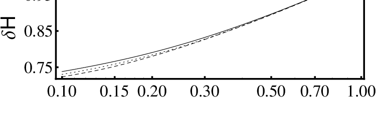
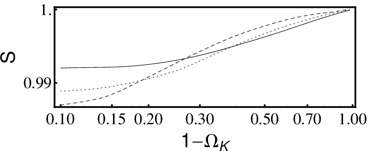
The LTB space-time is fully determined by a choice of the three free functions $k(r)$, $m(r)$ and $t_{0}(r)$. The first two of these are specified above, and the third is the ‘bang time’, which in these models need not be the same at all points in space. Without loss of generality, we can then make a coordinate choice such that $m=$constant. We will also initially consider the situation of a simultaneous big bang, with $t_{0}=$constant. These models have been much studied recently, as a space-time with local negative curvature allows for the possibility of explaining the supernova data without Dark Energy. A fit to the data is often found to be a void with $\Omega_{k}\sim 0.7$, and a width of $z\sim 0.5$. This is a significant amount of spatial curvature, extending out to large distances, and one may naively suspect that the sensitivity of the small angle CMB to spatial curvature may be sufficient to impose strong constraints on these models [9]-[13].

To investigate if this is indeed so, let us consider a negative local curvature fluctuation in an otherwise flat universe. An observer at the centre of such a void will see a last scattering surface at $z_{*}$, and can straightforwardly calculate $H$ at this surface in terms of their locally measured value. We also require a fiducial observer in an FRW universe who will witness an identical last scattering surface, with the same $H_{LS}$. To ensure that these observers use comparable measures of distance we will enforce the conditions that they have the same local geometry [21]. This choice ensures that distances to nearby co-moving objects are the same when measured in units of $h^{-1}$MPc. We also require that they both see last scattering surfaces at the same $z_{*}$ so that effects due to the redshifting of solid angle, for example, are automatically included.

The shift between the open FRW universe and the void model is then given by $S_{1}=d_{A,LS}^{\text{LTB}}/d_{A,LS}^{\text{open}}$, where the angular diameter distance in LTB is given by $d_{A,LS}^{\text{LTB}}=a_{1,LS}r_{LS}$, and in the FRW universe by Eq. (1). In the case of the void model, the values of $a_{1}$, $r$ and $H$ at last scattering are found by integrating a radial null geodesic out to $z_{*}$, using the solutions to Eq. (4). $H_{0}$ in the open FRW universe is then found by taking the same Hubble rate at last scattering as in the LTB model, and propagating it forward until today in the FRW geometry. Of course, we know the shift parameter between open and flat FRW universes, $S_{2}=d_{A,LS}^{\text{open}}/d_{A,LS}^{\text{EdS}}$ from (2), and so we can calculate the acoustic spectrum witnessed by the observer in the void in terms of a shift, $S=S_{1}S_{2}=d_{A,LS}^{\text{LTB}}/d_{A,LS}^{\text{EdS}}$, from a spatially flat FRW model, and a change in Hubble rate, $\delta H\equiv H_{0}^{EdS}/H_{0}^{LTB}$.

The shift, $S$, and change in Hubble rate, $\delta H$, for an asymptotically flat void formed from a negative Gaussian perturbation in $k(r)$, are shown in Fig. 2. We find that a good fit to the WMAP data requires $S\sim 0.9$ and $\delta H\sim 0.5$, and so a void model will need to be capable of achieving similar values if it is to be considered viable. It can immediately be seen that for moderately deep voids, with $\Omega_{k}\lesssim 0.9$ at the centre, both $S$ and $\delta H$ deviate insufficiently from $1$ [22]. It can also be seen that $S$ is not particularly sensitive to the width of the void. In light of what we considered above, these results can be easily understood: Most of the contribution to the shift does not come from the local geometry, but from early times when the CMB photons were well outside the void. The discussion above also explains why the presence of the void shifts the acoustic peaks to larger scales, rather than smaller.

One may also wish to consider more extreme voids in which we allow $\Omega_{k}>0.9$ at the centre. In this case, however, shell crossing singularities can occur [24], and redshift as a function of local energy density can become multi-valued [25]. The former of these should be considered as a break-down of the model, while the latter shows that the effect of the inhomogeneity on null geodesics in these cases can be highly non-trivial. However, even if one is prepared to consider such extreme voids, and even if they can be made compatible with the small angle CMB, such voids are still highly unlikely to be able to fit the supernova data without having their shape at low $z$ being highly fine-tuned. We will not consider them further here.

Of course, one will still be interested in more general void models. In particular, it is possible to conceive of a void in a spatially curved FRW universe, instead of a flat one. In this case one is subject to the familiar sensitivity of the CMB to spatial curvature, and we have verified that $S$ can effectively be set to any value with a suitable choice of asymptotic curvature [27]. In particular, a shift parameter of $S\simeq 0.9$ can be achieved with $\Omega_{k}\simeq-0.26$ asymptotically. The value of $\delta H$, however, is not so sensitive to $k$ in the background space-time. To achieve $\delta H\sim 0.5$ one must therefore be prepared to abandon the notion of the big bang happening at the same time at all points in space. A larger contrast between local and asymptotic Hubble rates can then be straightforwardly achieved. To this end, we find that a Gaussian void embedded in a spatially curved universe with $\Omega_{k}=0.10$, that has a FWHM in $k$ at $z=0.34$, in $t_{0}$ at $z=0.80$, and with an age of the universe in the centre of the void that is $13\%$ more than that of the asymptotic regions, we can fit the $C_{\ell}$s just as well as $\Lambda$CDM with $\Omega_{m}=0.15$ at the centre of the void. The CMB acoustic spectrum and distance modulus plot for this void are shown in Fig. 3, together with the $\Lambda$CDM best fits. Changing the detailed shape of the under-density will change the numbers involved above, and, in particular, if one can find other voids that allow $\delta H\sim 0.5$ then these models will very likely provide a good fit to the data too (with the appropriate choice of background curvature, to give the correct shift).

In conclusion, we find that the observed acoustic spectrum of small angle CMB fluctuations is primarily only sensitive to curvature at high redshifts. Local curvature has much smaller, and even opposite, effects. By considering LTB models, in which $k=k(r)$, we demonstrate that large local fluctuations in spatial curvature produce only moderate shifts in the CMB acoustic spectrum. As a result, the local void models that seek to explain cosmological observations without Dark Energy are not automatically ruled out. Fitting to the WMAP 5 year data shows, however, that the simplest voids (with simultaneous big bang) are required to be have non-zero asymptotic spatial curvature. By embedding the void in a suitably curved background it is then possible to shift the acoustic spectrum by any amount. Even in this case, however, the locally observed Hubble rate in the void model is anomalously low. Alternatively, we can give up on the idea of a simultaneous big bang. In this case it is found that the local Hubble rate (as well as the shift parameter) is sensitive to the bang time function, and by altering the age of the Universe in different spatial locations we can increase $H_{0}$. We therefore find void models that can fit the WMAP 5 year data just as well as $\Lambda$CDM, as well as local measurements of $H_{0}$, and supernova observations. However, if we really do live in a large, local under-density in the Universe, it will have to be considerably more complex than previously thought in order to be observationally viable.

References

- [1] Miller, A. et al ApJ Supp. 140, 115 (2002); Hanany, S. et al ApJ 545, L5 (2002); de Bernardis, P. et al Nature 404, 955 (2000); Dunkley, J. et al, Astrophys. J. Suppl. 180, 306 (2009).
- [2] Tomita, K. ApJ 451, 1 (1995) [Errata ApJ 464, 1054 (1996)]; ApJ 461, 507 (1996); Gen. Rel. Grav. 29, 815 (1997); Phys. Rev. D56, 3341 (1997); ApJ 529, 26 (2000); ApJ 529, 38 (2000).
- [3] Mustapha, N., Hellaby, C. & Ellis, G. MNRAS 292, 817 (1997).
- [4] Celerier, M. & Schneider, J. Phys. Lett. A249, 37 (1998).
- [5] Joyce, M. et al Europhys. Lett. 49, 416 (2000).
- [6] Tomita, K. MNRAS 326, 287 (2001).
- [7] Tomita, K. Prog. Theo. Phys. 106, 929 (2001).
- [8] Iguchi, H., Nakamura, T. & Nakao, K. Prog. Theo. Phys. 108, 809 (2002).
- [9] Alexander, S., Biswas, T. & Notari, A. JCAP 0909, 025 (2009).
- [10] Alnes, H., Amarzguioui, M. & Grøn, Ø. Phys. Rev.D73, 083519 (2006).
- [11] Alnes, H. & Amarzguioui, M. Phys. Rev. D74, 103520 (2006).
- [12] Garcia-Bellido, J. & Haugboelle, T. JCAP 04, 003 (2008).
- [13] Zibin, J., Moss, A. & Scott, D. Phys. Rev. Lett. 101, 251303 (2008).
- [14] Clifton, T., Ferreira, P. G. & Land, K. Phys. Rev. Lett. 101, 131302 (2008).
- [15] Tomita, K. arXiv:0906.1325.
- [16] Jungman, G. et al Phys. Rev. D54, 1332 (1996).
- [17] Gouda, N., Sugiyama, N. & Sasaki, M. Prog. Theor. Phys. 85, (1991).
- [18] This is not true of Baryon Acoustic Oscillations (BAOs) when the Universe is inhomogeneous. The curvature in the background will affect the position and amplitude of the oscillations in the galaxy power spectrum in a far more complicated way. Hence we do not use BAOs.
- [19] Kamionkowski, M., Spergel, D. & Sugiyama, N. Ap. J. 426, L57 (1994).
- [20] Lemaître, G. Ann. Soc. Sci. Brussels A53, 51 (1933); Tolman, R. Proc. Nat. Acad. Sci. USA 20, 169 (1934); Bondi, H. MNRAS 107, 410 (1947).
- [21] For non-singular voids it can be shown that the geometry at the centre is locally Friedman. See Bonnor, W. MNRAS 167, 55 (1974).
- [22] This is due to the value of , from Fig. 1, being largely cancelled by the value of , leaving .
- [23] Lewis, A. & Bridle, S. Phys. Rev. D66, 103511 (2002).
- [24] Shell crossing occurs when , and indicates a breakdown of the model due to the neglect of pressure in the matter content.
- [25] Moss, A., Zibin, J., & Scott, D., Phys. Rev. D83, 103515 (2011).
- [26] Freedman, W. et al Ap. J. 553, 47 (2001).
- [27] This may explain how the “unconstrained” models of [13] were able to produce a suitable fit to the data, albeit with low , as these models have a region of outside the central under-density.
- [28] Astier, P. et al Astron. Astrophys. 447, 31 (2006).