Fountain Codes Based Distributed Storage Algorithms for Large-scale
Wireless Sensor Networks

Our wireless sensor network consists of $n$ nodes that are uniformly distributed at random in a region $\mathcal{A}=[L,L]^{2}$ for $L>1$. The density of the network is given by

where $|\mathcal{A}|$ is the two-dimensional Lebesgue measure (or area) of ${\cal A}$. Each sensor node has an identical communication radius $1$; thus any two nodes can communicate with each other if and only if their distance is less than or equal to 1. This model is known as random geometric graphs [7, 15]. Among these $n$ nodes, there are $k$ source nodes that have information to be disseminated throughout the network for storage. These $k$ nodes are uniformly and independently distributed at random among the $n$ nodes. Usually, the fraction of source nodes, i.e., $\frac{k}{n}$, is not very large (e.g., $10\%$, or $20\%$).

Note that, although we assume the nodes are uniformly distributed at random in a region, our algorithms and results do not rely on this assumption. In fact, they can be applied for any network topology, for example, regular grids.

We assume that no node has knowledge about the locations of other nodes and no routing table is maintained; consequently, the algorithm proposed in [5] cannot be applied. Moreover, we assume that each node has limited or no knowledge of global information, but know its neighbors. The limited global information refers to the total numbers of nodes $n$ and sources $k$. Any further global information, for example the maximal number of neighbors in the network, is not available. Hence, the algorithms proposed in [11, 10] are not applicable.

For $k$ source blocks $\{x_{1},x_{2},\ldots,x_{k}\}$ and a probability distribution $\Omega(d)$ with $1\leq d\leq k$, a Fountain code with parameters $(k,\Omega)$ is a potentially limitless stream of output blocks $\{y_{1},y_{2},...\}$. Each output block is obtained by XORing $d$ randomly and independently chosen source blocks, where $d$ is drawn from a specially designed distribution $\Omega(d)$. This is illustrated in Figure 1. Fountain codes are rateless, and one of their main advantage is that the encoding operations can be performed online. The encoding cost is the expected number of operation sufficient for generating an output symbol, and the decoding cost is the expected number of operations sufficient to recover the $k$ input blocks. Another advantage of Fountain codes, as opposed to purely random codes is that their decoding complexity can be made low by appropriate choice of $\Omega(d)$, with little sacrifice in performance. The decoding of Fountain codes can be done by message passing.

LT (Luby Transform) codes are a special class of Fountain codes which uses Ideal Soliton or Robust Soliton distributions [12]. The Ideal Soliton distribution $\Omega_{is}(d)$ for $k$ source blocks is given by

Let $R=c_{0}\sqrt{k}\ln(k/\delta)$, where $c_{0}$ is a suitable constant and $0<\delta<1$. The Robust Soliton distribution for $k$ source blocks is defined as follows. Define

and let

The Robust Soliton distribution is given by

The following result provides the performance of the LT codes with Robust Soliton distribution [12, Theorems 12 and 13].

In LTCDS-I, we assume that each node in the network knows the values of $k$ and $n$. We use simple random walks [1, 17] for each source to disseminate its information to the whole network. At each round, each node $u$ that has packets to transmit chooses one node $v$ among its neighbors uniformly independently at random, and sends the packet to the node $v$. In order to avoid local-cluster effect—each source packet is trapped most likely by its neighbor nodes—we let each node accept a source packet equiprobably. To achieve this, we also need each source packet to visit each node in the network at least once.

For a random walk on a graph, the cover time is defined as follows [1, 17]:

For a simple random walk on a random geometric graph, the following result bounds the cover time [3].

As a result of Lemma 5, we can set a counter for each source packet and increase the counter by one after each forward transmission until the counter reaches some threshold $C_{1}n\log n$ to guarantee that the source packet visits each node in the network at least once. The detailed descriptions of the initialization, encoding and storage phases (steps) of LTCDS-I algorithm are given below:

1. (i)

   Initialization Phase:

   1. (1)

      Each node $u$ in the network draws a random number $d_{c}(u)$ according to the distribution $\Omega_{is}(d)$ given by (3) (or $\Omega_{rs}(d)$ given by (6)). Each source node $s_{i},i=1,\dots,k$ generates a header for its source packet $x_{s_{i}}$ and puts its ID and a counter $c(x_{s_{i}})$ with initial value zero into the packet header. We set up tokens for initial and update packets. We assume that a token is set to zero for an initial packet and $1$ for an update packet.

      $$packet_{s_{i}}=(ID_{s_{i}},x_{s_{i}},c(x_{s_{i}}))$$

   2. (2)

      Each source node $s_{i}$ sends out its own source packet $x_{s_{i}}$ to another node $u$ which is chosen uniformly at random among all its neighbors $\mathcal{N}(s_{i})$.

   3. (3)

      The chosen node $u$ accepts this source $packet_{s_{i}}$ with probability $\frac{d_{c}(u)}{k}$ and updates its storage as

      $$y_{u}^{+}=y_{u}^{-}\oplus x_{s_{i}},$$

      (9)

      where $y_{u}^{-}$ and $y_{u}^{+}$ denote the packet that the node $u$ stores before and after the updating, respectively, and $\oplus$ represents XOR operation. No matter whether the source packet is accepted or not, the node $u$ puts it into its forward queue and set the counter of $x_{s_{i}}$ as

      $$c(x_{s_{i}})=1.$$

      (10)

2. (ii)

   Encoding Phase:

   1. (1)

      In each round, when a node $u$ receives at least one source packet before the current round, $u$ forwards the head-of-line (HOL) packet $x$ in its forward queue to one of its neighbor $v$, chosen uniformly at random among all its neighbors $\mathcal{N}(u)$.

   2. (2)

      Depending on how many times $x$ has visited $v$, the node $v$ makes its decisions:

      1. •

         If it is the first time that $x$ visits $v$, then the node $v$ accepts this source packet with probability $\frac{d}{k}$ and updates its storage as

         $$y_{v}^{+}=y_{v}^{-}\oplus x.$$

         (11)

      2. •

         If $x$ has visited $v$ before and $c(x)<C_{1}n\log n$ where $C_{1}$ is a system parameter, then the node $v$ accepts this source packet with probability 0.

      3. •

         No matter $x$ is accepted or not, the node $v$ puts it into its forward queue and increases the counter of $x$ by one:

         $$c(x)=c(x)+1.$$

         (12)

      4. •

         If $x$ has visited $v$ before and $c(x)\geq C_{1}n\log n$ then the node $v$ discards the packet $x$ forever.

3. (iii)

   Storage Phase:

   When a node $u$ makes its decisions for all the source packets $x_{s_{1}},x_{s_{2}},...,x_{s_{k}}$, i.e., all these packets have visited the node $u$ at least once, the node $u$ finishes its encoding process by declaring the current $y_{u}$ to be its storage packet.

The pseudo-code of these steps is given in LTCDS-I Algorithm 1.

The following theorem establishes the code degree distribution of each storage node induced by the LTCDS-I algorithm.

Theorem 6 indicates that the code degree $\tilde{d}_{c}(u)$ is not the same as $d_{c}(u)$. In fact, one may achieve the exact desired code degree distribution by letting all the sensors hold the received source packets in their temporary buffer until they collect all $k$ source packets. Then they can randomly choose $d_{c}(u)$ packets. In this way, the resulting degree distribution is exactly the same as $\Omega_{is}$ or $\Omega_{rs}$. However, this requires that each sensor has enough buffer or memory, which is usually not practical, especially when $k$ is large. Therefore, in LTCDS-I, we assume each sensor has very limited memory and let them make their decision upon each reception.

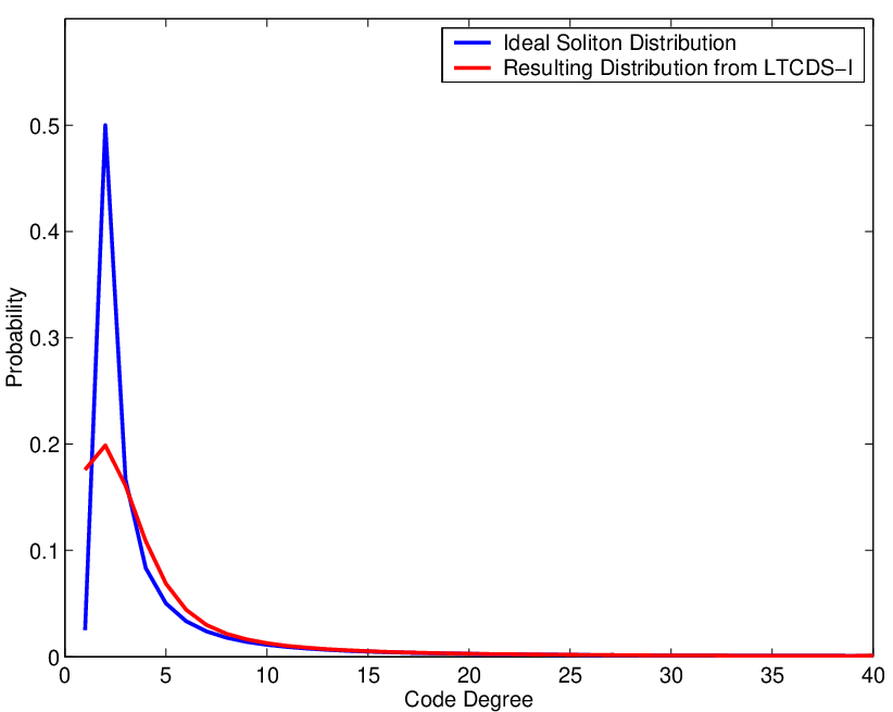
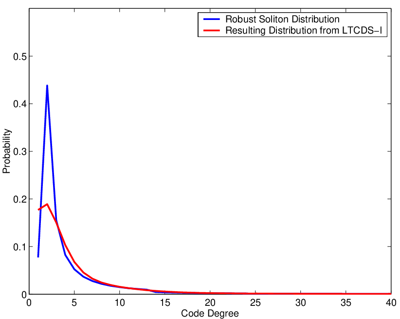
Fortunately, from Figure 2, we can see that at the high degree end, the resulting code degree distribution obtained by the LTCDS-I algorithm (13) perfectly matches the desired code degree distribution, i.e., either the Ideal Soliton distribution $\Omega_{is}$ (3) or the Robust Soliton distribution $\Omega_{rs}$ (6). For the resulting degree distribution and the desired degree distributions, the difference only lies at the low degree end, especially at degree 1 and degree 2. In particular, the resulting degree distribution has higher probability at degree 1 and lower probability at degree 2 than the desired degree distributions. The fact that higher probability at degree 1 turns out to compensate the lower probability at degree 2 so that the resulting degree distribution has very similar encoding and decoding behavior as LT codes using either the Ideal Soliton distribution or the Robust Soliton distribution. In our future study, we will provide theoretical analysis and prove that the degree distribution in 13 is equivalent, but not the same, as the degree distributed used in LT encoding [12]. Therefore, we have the following theorem, which can be proved by the same method for Lemma 3, see [12].

Theorem 7 asserts that when $n$ and $k$ are sufficiently large, the performance of the LTCDS-I is similar to LT coding.

Another main performance metric is the transmission cost of the algorithm, which is characterized by the total number of transmissions (the total number of steps of $k$ random walks).

In many scenarios, especially when a change in network topology occurs because of, for example, node mobility or node failures, the exact values of $n$ and $k$ may not be available to all nodes. Therefore, to design a fully distributed storage algorithm which does not require any global information is very important and useful. In this subsection, we present such an algorithm based on LT codes, called LTCDS-II. The idea behind this algorithm is to utilize some features of simple random walks to do inference to obtain individual estimates of $n$ and $k$ for each node.

We introduce of inter-visit time and inter-packet time [1, 17, 14] as follows:

For a simple random walk on random geometric graphs, the following lemma provides results on the expected inter-visit time of any node. The proof is straightforward by following the standard result of stationary distribution of a simple random walk on graphs and the mean return time for a Markov chain [1, 17, 14]. For completeness, we provide the proof in Appendix 6.1.

From Lemma 10, we can see that if each node $u$ can measure the expected inter-visit time $E[T_{visit}(u)]$, then the total number of nodes $n$ can be estimated by

However, the mean degree $\mu$ is a global information and may be hard to obtain. Thus, we make a further approximation and let the estimate of $n$ by the node $u$ be

Hence, every node $u$ computes its own estimate of $n$. In our distributed storage algorithms, each source packet follows a simple random walk. Since there are $k$ sources, we have $k$ individual simple random walks in the network. For a particular random walk, the behavior of the return time is characterized by Lemma 10. On the other hand, Lemma 12 below provides results on the inter-visit time among all $k$ random walks, which is called inter-packet time for our algorithm, defined as follows:

For the mean value of inter-packet time, we have the following lemma, for which the proof is given in Appendix 6.2.

From Lemma 10 and Lemma 12, it is easy to see that for any node $u$, an estimation of $k$ can be obtained by

After obtaining estimates for both $n$ and $k$, we can employ similar techniques used in LTCDS-I to do LT coding and storage. The detailed descriptions of the initialization, inference, encoding, and storage phases of LTCDS-II algorithm are given below:

1. (i)

   Initialization Phase:

   1. (1)

      Each source node $s_{i},i=1,\dots,k$ generates a header for its source packet $x_{s_{i}}$ and puts its ID and a counter $c(x_{s_{i}})$ with initial value zero into the packet header.

   2. (2)

      Each source node $s_{i}$ sends out its own source packet $x_{s_{i}}$ to one of its neighbors $u$, chosen uniformly at random among all its neighbors $\mathcal{N}(s_{i})$.

   3. (3)

      The node $u$ puts $x_{s_{i}}$ into its forward queue and sets the counter of $x_{s_{i}}$ as

      $\displaystyle c(x_{s_{i}})=1.$

      (20)

2. (ii)

   Inference Phase:

   1. (1)

      For each node $u$, suppose $x_{s(u)_{1}}$ is the first source packet that visits $u$, and denote by $t_{s(u)_{1}}^{(j)}$ the time when $x_{s(u)_{1}}$ has its $j$-th visit to the node $u$. Meanwhile, each node $u$ also maintains a record of visiting time for each other source packet $x_{s(u)_{i}}$ that visited it. Let $t_{s(u)_{i}}^{(j)}$ be the time when source packet $x_{s(u)_{i}}$ has its $j$-th visit to the node $u$. After $x_{s(u)_{1}}$ visiting the node $u$ $C_{2}$ times, where $C_{2}$ is system parameter which is a positive constant, the node $u$ stops this monitoring and recoding procedure. Denote by $k(u)$ the number of source packets that have visited at least once upon that time.

   2. (2)

      For each node $u$, let $J(s(u)_{i})$ be the number of visits of source packet $x_{s(u)_{i}}$ to the node $u$ and let

      	$\displaystyle\!\!T_{s(u)_{i}}\!\!$	$\displaystyle=$	$\displaystyle\!\!\!\!\frac{1}{J(s(u)_{i})}\!\!\!\sum_{j=1}^{J(s(u)_{i})}t_{s(u)_{i}}^{(j+1)}-t_{s(u)_{i}}^{(j)}$		(21)
      		$\displaystyle=$	$\displaystyle\!\!\!\!\frac{1}{J(s(u)_{i})}(t_{s(u)_{i}}^{(J(s(u)_{i}))}-t_{s(u)_{i}}^{(1)}).$		(22)

      Then, the average inter-visit time for node $u$ is given by

      $$\bar{T}_{visit}(u)=\frac{1}{k(u)}\sum_{i=1}^{k(u)}T_{s(u)_{i}}.$$

      (23)

      Let $J_{min}=\min_{s(u)_{i}}\{t_{s(u)_{i}}^{(1)}\}$ and $J_{max}=\max_{s(u)_{i}}\{t_{s(u)_{i}}^{(J(s(u)_{i}))}\}$, then the inter-packet time is given by

      $$\bar{T}_{packet}(u)=\frac{J_{min}-J_{max}}{\sum_{s(u)_{i}}J(s(u)_{i})}.$$

      (24)

      Then the node $u$ can estimate the total number of nodes in the network and the total number of sources as

      $$\hat{n}(u)=\bar{T}_{visit}(u),$$

      (25)

      and

      $$\hat{k}(u)=\frac{\bar{T}_{visit}(u)}{\bar{T}_{packet}(u)}.$$

      (26)

   3. (3)

      In this phase, the counter $c(x_{s_{i}})$ of each source packet $c(x_{s_{i}})$ is incremented by one after each transmission.

3. (iii)

   Encoding Phase:

   When a node $u$ obtains estimates $\hat{n}(u)$ and $\hat{k}(u)$, it begins encoding phase which is the same as the one in LTCDS-I Algorithm except that the code degree $d_{c}(u)$ is drawn from distribution $\Omega_{is}(d)$ (or $\Omega_{rs}(d)$) with replacement of $k$ by $\hat{k}(u)$, and a source packet $x_{s_{i}}$ is discarded if $c(x_{s_{i}})\geq C_{3}\hat{n}(u)\log\hat{n}(u)$, where $C_{3}$ is a system parameter which is a positive constant.

4. (iv)

   Storage Phase:

   When a node $u$ has made its decisions for $\hat{k}$ source packets, it finishes its encoding process and $y_{u}$ becomes the storage packet of $u$.

The total number of transmissions (the total number of steps of $k$ random walks) in the LTCDS-II algorithm has the same order as LTCDS-I.

Now, we turn our attention to data updating after all storage nodes saved their values $y_{1},y_{2},\ldots,y_{n}$, but a sensor node, say $s_{i}$, wants to update its value to the appropriate set of storage nodes in the network. The following updating algorithm applies for both LTCDS-I and LTCDS-II. For simplicity, we illustrate the idea with LTCDS-I.

Assume the sensor node prepared a packet with its ID, old data $x_{s_{i}}$, new data $x^{\prime}_{s_{i}}$ along with a time-to-live parameter $c(s_{i})$ initialized to zero. We will use also a simple random walk for data update.

If we assume that the storage nodes keep ID’s of the accepted packets, then the problem becomes simple. We just run a random walk and check for the coming packet’s $ID$. Assume the node $u$ keeps track of all $ID$’s of its accepted packets. Then $u$ accepts the updated message if $ID$ of the coming packet is already included in the $u$’s $ID$ list. Otherwise $u$ forwards the packet incrementing the time-to-live counter. If this counter reaches the threshold value, then the packet will be discarded.

The following steps describe the update scenario:

1. (i)

   Preparation Phase:

   The node $s_{i}$ prepares its new packet with the new and old data along with its ID and counter. Also, $s_{i}$ add an update counter $token$ initialized at $1$ for the first updated packet. So, we assume that the following steps happen when $token$ is set to $1$.

   $\displaystyle packet_{s_{i}}=(ID_{s_{i}},x_{s_{i}}\oplus x^{\prime}_{s_{i}},c(s_{i})).$

   (29)

   $s_{i}$ chooses at random a neighbor node $u$, and sends its $packet_{s_{i}}$.

2. (ii)

   Encoding Phase:

   The node $u$ checks if the $packet_{s_{i}}$ is an update or first-time packet. If it is first-time packet it will accept, forward, or discard it as shown in LTCDS-I algorithm 1. If $packet_{s_{i}}$ is an updated packet, then the node $u$ will check if $ID_{s_{i}}$ is already included in its accepted list. If yes, then it will update its value $y_{u}$ as follows.

   $\displaystyle y_{u}^{+}=y_{u}^{-}\oplus x_{s_{i}}\oplus x_{s_{i}}^{\prime}.$

   (30)

   If no, it will add this updated packet into its forward queue with incrementing the counter

   $\displaystyle c(x_{s_{i}}^{\prime})=c(x_{s_{i}}^{\prime})+1.$

   (31)

   The $packet_{s_{i}}$ will be discarded if $c(x_{s_{i}}^{\prime})\geq C_{1}n\log n$ where $C_{1}$ is a system parameter. In this case, we need $C_{1}$ to be large enough, so all old data $x_{s_{i}}$ will be updated to the new data $x_{s_{i}}^{\prime}$.

3. (iii)

   Storage Phase:

   If all nodes are done with updating their values $y_{i}$. One can run the decoding phase to retrieve the original and update information.

Now, since we run only one simple random walk for each update, if $h$ is the number of nodes updating their values, then we have the following result.

References

- [1] D. Aldous and J. Fill. Reversible Markov Chains and Random Walks on Graphs. Preprint, available at http://statwww.berkeley.edu/users/aldous/RWG/book.html, 2002.
- [2] S. A. Aly, Z. Kong, and E. Soljanin. Fountain codes based distributed storage algorithms. U.S. patent, Submitted, October, 2007.
- [3] C. Avin and G. Ercal. On the cover time of random geometric graphs. In Proc. 32nd International Colloquium of Automata, Languages and Programming, ICALP’05, Lisboa, Portugal, July, 2005.
- [4] A. G. Dimakis, V. Prabhakaran, and K. Ramchandran. Decentralized erasure codes for distributed networked storage. IEEE/ACM Transactions on Networking (TON), 14(SI):2809 – 2816, June 2006.
- [5] A. G. Dimakis, V. Prabhakaran, and K. Ramchandran. Ubiquitous access to distributed data in large-scale sensor networks through decentralized erasure codes. In Proc. of 4th IEEE Symposium on Information Processing in Sensor Networks (IPSN ’05), Los Angeles, CA, USA, April, 2005.
- [6] A. G. Dimakis, V. Prabhakaran, and K. Ramchandran. Distributed fountain codes for networked storage. Acoustics, Speech and Signal Processing, ICASSP 2006, may 2006.
- [7] E. N. Gilbert. Random plane networks. J. Soc. Indust. Appl. Math., 9:533–543, 1961.
- [8] A. Kamra, J. Feldman, V. Misra, and D. Rubenstein. Data persistence in sensor networks: Towards optimal encoding for data recovery in partial network failures. In Workshop on Mathematical performance Modeling and Analysis, June 2005.
- [9] A. Kamra, V. Misra, J. Feldman, and D. Rubenstein. Growth codes: Maximizing sensor network data persistence. In Proc. of the 2006 conference on Applications, technologies, architectures, and protocols for computer communications, Sigcomm06, pages 255 – 266, Pisa, Italy, 2006.
- [10] Y. Lin, B. Li, , and B. Liang. Differentiated data persistence with priority random linear code. In Proc. of 27th International Conference on Distributed Computing Systems (ICDCS’07), Toronto, Canada, June, 2007.
- [11] Y. Lin, B. Liang, and B. Li. Data persistence in large-scale sensor networks with decentralized fountain codes. In Proc. of the 26th IEEE INFOCOM07, Anchorage, Alaska, May 6-12, 2007.
- [12] M. Luby. LT codes. In Proc. 43rd Symposium on Foundations of Computer Science (FOCS 2002), 16-19 November 2002, Vancouver, BC, Canada, 2002.
- [13] D. S. Lun, N. Ranakar, R. Koetter, M. Medard, E. Ahmed, and H. Lee. Achieving minimum-cost multicast: A decentralized approach based on network coding. In In Proc. the 24th IEEE INFOCOM, volume 3, pages 1607– 1617, March 2005.
- [14] R. Motwani and P. Raghavan. Randomized Algorithms. Cambridge University Press, 1995.
- [15] M. Penrose. Random Geometric Graphs. Oxford University Press, New York, 2003.
- [16] M. Pitkanen, R. Moussa, M. Swany, and T. Niemi. Erasure codes for increasing the availability of grid data storage. In Proc. of the Advanced International Conference on Telecommunications and International Conference on Internet and Web Applications and Services (AICT/ICIW ), 2006.
- [17] S. Ross. Stochastic Processes. Wiley, New York, second edition, 1995.
- [18] I. Stojmenovic. Handbook of sensor networks, algorithms and architechtrues. Wiley series on parallel and distributed computing, 2005.