Compact shell solitons in field theories
Abstract
Some models providing shell-shaped static solutions with compact support (compactons) in 3+1 and 4+1 dimensions are introduced, and the corresponding exact solutions are calculated analytically. These solutions turn out to be topological solitons, and may be classified as maps and suspended Hopf maps, respectively. The Lagrangian of these models is given by a scalar field with a non-standard kinetic term ( field) coupled to a pure Skyrme term restricted to , rised to the appropriate power to avoid the Derrick scaling argument. Further, the existence of infinitely many exact shell solitons is explained using the generalized integrability approach. Finally, similar models allowing for non-topological compactons of the ball type in 3+1 dimensions are briefly discussed.
Keywords:
Compact solitons, Hopf maps1 Introduction
Recently, some effort has been invested into the investigation of compactons, that is, soliton solutions of non-linear field theories with compact support. By now, two established classes of scalar field theories are known which give rise to the existence of compacton solutions. One may either choose potentials in the Lagrangian (or energy density) which have a non-continuous first derivative at (some of) their minima [1] - [9], or one may employ a non-standard kinetic term ( field theory) [10], [11]. Concretely, the kinetic term has to contain higher than second powers in the first derivatives of the fields. For nonrelativistic field theories, compactons were first discovered and studied for some generalizations of the KdV equation in [12], [13]. Compactons can be realized directly in some mechanical systems [1], and, in addition, they have been applied recently to brane cosmology [14], [15], [16]. Most of these investigations have dealt with topological compactons, where the existence and stability of the compacton solutions is related to a nontrivial vacuum manifold and some nonzero topological charge. Also in this letter we shall mainly deal with this case of topological compactons, which turn out to have the shape of shells, and only at the end we will investigate a similar theory which, however, gives rise to non-topological compactons with a ball shape.
As is typical in soliton theory in general, it is easier to find systems with compacton solutions in low (that is 1+1) dimensions. The simplest, most obvious generalization of topological compacton systems with a non-standard kinetic term to higher dimensions meets the same obstacles as in the case of conventional solitons, and also the remedy to circumvent the obstacle is the same, namely the introduction of a gauge field in addition to the scalar fields, like in the case of vortices and monopoles [17]. In this letter, we shall pursue a different path for the construction of higher-dimensional topological compactons. Concretely, we couple a real scalar field with non-standard kinetic term to a complex scalar field where maps from a compact submanifold of the base space ( or for or , respectively) to an target space, thereby providing an important contribution to the non-trivial topology of the compacton solutions. The non-trivial topology is completed by the boundary conditions on required by finiteness of the energy. For the model constructed in Section 2, the complex scalar field has the topology of a Hopf map , and provides the suspension of this Hopf map to a map . The base space for this example is, therefore, 4+1 dimensional. In Section 3, we discuss similar models which allow for compactons in 3+1 dimensions, where describes a map . In Section 3.1, we study a model which again gives rise to analytical solutions which are shell-shaped. In Section 3.2 we introduce a slightly different model, where it turns out that the compact solitons are ball-shaped and, further, are no longer topological.
2 4-dimensional compactons
The specific dimensional model we are going to consider is given by the following expression
| (1) |
where etc. It describes a real scalar field with a non-standard kinetic term coupled to the pure Skyrme term constrained to target space
| (2) |
Here is a complex scalar providing via the stereographic projection a parametrisation of . This Lagrangian provides a simple, minimal generalization of the concept of fields to a model with target space. Here, minimal means that only one of the degrees of freedom is of the type. For different, non-minimal generalizations see e.g. [18], [19]. Observe that the above Lagrangian can also be derived by a reduction of a scalar field coupled to the standard non-abelian gauge field i.e., of -dilaton Yang–Mills theory. The coupling between both fields is of the non-minimal type and governed by the coupling function which is chosen in the form
| (3) |
Notice that the coupling function is semipositive definite and vanishes for
two values of the scalar field . Therefore, it plays the role
of an effective potential with two effective vacua for . The constant
is a free parameter of the model.
The pertinent field equations read
| (4) |
| (5) |
where
| (6) |
In order to derive static solutions we introduce the coordinates
| (7) |
where are coordinates on , and gives the extension to . Moreover, we assume the ansatz
| (8) |
and
| (9) |
This ansatz provides that
| (10) |
and, as a consequence, one can remove the coupling function from
equation (5). Equation (5) for the field simplifies,
in fact, to the field equation for the Lagrangian with base
space . Solutions to this model have been constructed in
[20], [21], and below we just review the results which we need
in the sequel.
Concretely, the static equations of motion may be rewritten in the form
| (11) |
| (12) |
The last expression may be simplified
| (13) |
Thus,
| (14) |
where is an integration constant. One can proceed further and solve this equation. However, for the topologically nontrivial configurations the complex field should cover the whole target space at least once. This requirement gives a condition for the integration constants leading to the solutions
| (15) |
In the case when we arrive at the very simply formula
| (16) |
Moreover, such a complex field being a map from (the base space parameterized by coordinates) to the target can be classified by a topological invariant known as the Hopf index. In fact, solution (8), with (15), (16) is known to carry a non-vanishing Hopf index
| (17) |
Let us now turn to the field equation for the real scalar . First of all one can observe that this expression leads to an ordinary differential equation for only if in the solution for the . Therefore, only the solution (16) is admissible. Then, the -dependence in the second term of (11) cancels and we get
| (18) |
Introducing the new variable we find that
| (19) |
This equation has been recently analyzed in the context of compact domain walls [10]. The corresponding compacton solution located at reads
| (20) |
where
| (21) |
Finally, the 4 dimensional compacton solution is
| (22) |
(where ), together with
| (23) |
with the Hopf index of the underlying Hopf maps equal to .
The size of the compact soliton, if treated as an object living in the
original 4 dimensional space, varies as one changes its position. The
inner and outer compacton boundary points
are
| (24) |
where gives a parametrisation of the center of the solution. Thus the shell radius is
| (25) |
As we see, the compacton is getting narrower as it approaches the origin. On
the other hand its radius grows while it moves in the opposite direction.
The energy of the solution is given as follows
| (26) |
Thus,
| (27) |
| (28) |
It is clearly visible that the compact solution for the real scalar field is of
the Bogomolny type, satisfying a first order differential equation, which may
be easily derived from (28) using the standard Bogomolny trick.
Specifically, for the one-compacton configuration we find
| (29) |
Interestingly, the energy depends on a non-integer power of the
Hopf charge of the underlying
field, like in the Vakulenko-Kapitansky formula [22].
It should be mentioned, however, that this relation between energy and Hopf
charge does not provide an energy bound for general Hopf charge, because the
full field configuration is a suspended Hopf map, and its topological
classification is therefore given by the homotopy group , as we demonstrate below.
So let us prove that the obtained configuration may be understood as a
suspended Hopf map, i.e., a map from the base space onto the target
space characterized by the nontrivial homotopy class . It is
convenient to combine the fields into a matrix
| (30) |
where
| (31) |
and is the unit matrix. Thus, the field maps onto the three
dimensional target sphere. For every fixed value of
the field
is just a Hopf map with the previously found nonvanishing
topological charge. For , representing the poles of , we
get the identity map. Therefore we get a full covering of the . The
boundary condition, as , allows
for compactification of the original space to . These facts
render the a representative of the nontrivial homotopy class
[23]. We remark
that topological solitons which may be classified as suspended Hopf maps
(although not of the compacton type) have been studied recently, e.g., in
[24] and in [25].
Interestingly, the compactons we found do not have the structure of a ball.
Instead, they have the form of a shell, where the energy density is radially
symmetric, and is zero both inside the inner compacton boundary and outside
the outer boundary. Further,
the one compacton solution may be easily extended to multi-compacton
configurations
by taking an alternating collection of sufficiently separated compactons
(which interpolate from the vacuum value to with
increasing radius)
and
anti-compactons
(which interpolate from to with increasing radius),
forming an onion-like structure with one compacton or
anti-compacton as the innermost shell, surrounded by further compacton and
anti-compacton shells. The energy of the solution equals just the sum of
the energies of all compact solitons. The corresponding topological charge
is nontrivial if the number of compactons is not the same as the number of
anticompactons, whereas it is zero if the number of compactons and
anti-compactons is equal. We remark that the Hopf charge of the field
within each (anti-)compacton may be chosen independently.
Let us also notice that the simplest compact Hopf map is stable as far as
linear radial perturbations are considered. In this case the
stability analysis of [10], [14], [15] holds.
The existence of infinitely many exact suspended
hopfion solutions in our model makes it interesting to further investigate its integrability properties. First we observe that the model has infinitely many symmetries and, therefore, infinitely many conserved currents. The symmetries are just the area-preserving diffeomorphisms acting on the target space spanned by the complex scalar field , and the conserved currents are the corresponding Noether currents. One way to further analyse the integrability
is provided by the generalized zero curvature condition of Refs. [26],
[27], which gives a well-defined extension of the standard
integrability criterion (Zakharov-Shabat zero curvature representation) to higher
than two dimensions. The corresponding generalized zero curvature condition
is the condition for the holonomy in higher loop space to be independent
of the deformations of loops or, in other words, it is just a condition for
the flatness of the connetion in loop space. Moreover, assuming the
reparametrization invariance of the holonomy, one gets local generalized
zero curvature conditions,
| (32) |
i.e., flatness of a connetion and covariant
constancy of a vector field , where is
a Lie algebra and an abelian ideal (a representation space of
the Lie algebra). A model is said to be integrable if one can rewrite the
field equations as the generalized zero curvature conditions (32) and
if the abelian ideal used in the construction has infinite dimensions.
One can verify that the model (1) admits such a generalized zero
curvature formulation provided we impose an additional constraint on the
fields. Therefore our model, although not integrable in this sense, possesses an
integrable sector defined by the following integrability condition
| (33) |
In particular, the generalized zero curvature formulation of the submodel is given by
| (34) |
| (35) |
where are the generators of the Lie algebra and
transforms under the spin- representation of . The
equations of motion for the submodel are given by GZC in any spin
representation, which implies the generalized integrability. The importance
of this submodel emerges from the fact that our hopfions belong to it.
Indeed, they solve the field equation together with the constraint.
One can compare the integrability properties of our model with the most known example of target space model i.e., the Skyrme model. The Skyrme model does not have infinitely many symmetries, but it also has an integrable sector. However, in this case it is given by two integrability conditions
| (36) |
Thus, the integrable submodel is much more constrained, and this fact obviously affects the chance for the existence of exact solitons. In particular, the new condition, that is, the eikonal equation, is rather restrictive. It leads to one exact, given solution once the nontrivial topology (the Hopf charge) for is fixed (more precisely, it leads to one fixed solution up to Moebius transformations, that is, rotations of the target space where takes its values). This is in contrast to the first integrability condition, which is easily obeyed by a general separation of variables ansatz. This can explain why our model as well as its extention presented in the next section possess infinitely many exact solutions based on infinitely many Hopf maps
(or infinitely many maps in the next section).
The relation between the restrictions imposed by the integrability conditions and existence of exact solutions is also confirmed by recent investigations of the pure quartic (Euclidean) Skyrme model by Speight [22]. In fact, in this model, which from the point of view of the generalized integrability is exactly the same as the Skyrme model, only one exact soliton with topology of the suspended hopfion has been found. It is not of the compacton type.
3 Some 3-dimensional compactons
Here we want to study briefly some models which give rise to compacton solutions analogous to the case discussed in the preceding section, but in 3+1 dimensions, which is the case more directly relevant for physical applications. We shall discuss explicitly two cases.
3.1 Shell-shaped compactons
In the first example, we observe that the Lagrangian (1) of Section 2 is quartic in first derivatives, therefore it is scale invariant precisely in four dimensions, which is one way to circumvent Derrick’s theorem and have static solutions in four dimensions. If we want to have static solutions in three dimensions, one possibility consists, therefore, in choosing a Lagrangian cubic in first derivatives. This implies, however, that the resulting Lagrangian is non-polynomial. For models of this type the study of time-dependent dynamics is problematic (e.g. boundedness of the energy, or global hyperbolicity), therefore we shall introduce the energy functional for static configurations directly. Concretely, the three-dimensional model we study has the following energy functional for static configurations
| (37) |
where . It is related to the model (1) of Section 2 such that both terms of the model (1) are taken to the power . Further, we have already reduced to the static case. If we now introduce three-dimensional spherical polar coordinates and use the ansatz , , then the coupling function can again be removed from the equation for , and this equation can be written as
| (38) |
This equation is just the field equation of the model of Aratyn, Ferreira and Zimermann (AFZ)11 1 The energy density is, in fact, precisely the energy density of the AFZ model. In three-dimensional, Euclidean base space, the AFZ model has infinitely many soliton solutions of the knot type [28], [29], whose existence is related both to the conformal base space symmetry and to the infinitely many target space symmetries of this model. Here we are, however, interested in solutions on the base space .. For the ansatz it has the solutions
| (39) |
where is an integer and these solutions describe maps with winding number . The corresponding reads
| (40) |
The equation for for this ansatz is
| (41) |
or, for the specific coupling function and the above,
| (42) |
Introducing again the variable , this equation becomes
| (43) |
which has exactly the same compacton solution (20) as in Section 2, where now the constant is
| (44) |
Therefore, this model has exactly the same shell-like
spherically symmetric compacton solutions in
three dimensions as the previous model of section 2 has in four dimensions.
The topology of the compacton solutions is now given by maps .
This topology may again be described by the SU(2) matrix of Eq.
(30), where, however, now the complex scalar is a map .
Therefore, the solution field configuration takes its value at the north pole
of the target space for (inside the inner shell boundary),
covers the full target while varies from to ,
and takes its value at the south pole for (outside the outer shell
boundary).
Also the integrability properties are exactly equivalent to the ones of the model of Section 2.
The present model has infinitely many symmetries and infinitely many conserved currents,
like the one of Section 2. Further, the generalized zero curvature representation does not exist
for the full model, but only for a submodel defined by the additional condition (33),
again in complete analogy with the model of Section 2.
3.2 Ball-shaped compactons
Another simple modification which allows for compactons in three spatial dimensions is given by the Lagrangian
| (45) |
Here, the term
| (46) |
is just the Lagrangian of the CP1 model. The above Lagrangian contains one
quartic term and one quadratic term in first derivatives, and so may have
finite energy solutions in three dimensions, according to the Derrick scaling
argument.
It is, however, not scale invariant nor does it have infinitely many
symmetries, in contrast to the models studied above. Therefore, we do not
expect to find fully analytical solutions in this case, see below.
We again use the ansatz , in spherical polar coordinates in three
space dimensions. With this ansatz, the coupling function may again be eliminated from the field equation for , and this
equation is, therefore, just the field equation of the CP1 model on base
space . The simplest solution of this equation is
| (47) |
The CP1 energy density of this solution is
| (48) |
There exist many more solutions of the CP1 model like, e.g., higher powers of the simplest solution, but the corresponding energy densities are no longer independent of the angular coordinates. These higher solutions are, therefore, not compatible with our separation ansatz , and we have to restrict to the simplest solution (47) in what follows. For this simplest CP1 solution, we find the following Euler–Lagrange equation for
| (49) |
or, after the variable transformation
| (50) |
This equation differs from the previous ones by the explicit presence of the
factor (the independent variable) in the second term, that is, it is no
longer an autonomous equation. As expected, we were not able to find
analytic solutions to this equation, so we will resort to a qualitative
analysis and to a numerical study in the sequel. Further,
we shall find that its solutions are
no longer topological and may, therefore, have arbitrarily small energies.
Concretely, a numerical integration of Eq. (50) leads to the following
results:
- •
There do not exist shell-type solutions. If one starts the integration at an inner boundary with taking one vacuum value (e.g. ), and , then the integration into the direction never reaches the other vacuum value . Instead, a point is reached where and , and at this point becomes singular (it is obvious from Eq. (50) that at a point where , either must take one of its vacuum values, or becomes singular).
- •
There exist, however, solutions of the ball type. If one starts the numerical integration at an outer compacton boundary (e.g., with and ) and integrates towards , then the integration will simply hit the point . In order to see that the resulting solution is an acceptable compacton, it is more useful to reverse the integration and to start at .
- •
Let us assume that we start the integration at with some value and with . First, we observe that due to the suppression factor in the second term of Eq. (50), and may take arbitrary values without making singular (concretely, if then ). For , we note that for it holds that , whereas for it holds that , as follows easily from Eq. (50).
- •
Therefore, with the initial conditions given above, the following picture emerges for an integration starting at . If is too large, then the integration curve for will cross the line and then grow forever, producing a formal solution with infinite energy. If is too small, the integration curve will reach a point where but still . At this point the integration curve becomes singular, because is singular. It follows that there exists a fine tuned value for the integration constant such that the integration curve touches the line instead of crossing it, that is, it reaches the value precisely at the point where . This configuration is the compacton. The above qualitative discussion is completely confirmed by an explicit numerical integration.
In the above argument, we could start the integration at for an
arbitrary value . By choosing a arbitrarily close
to the value we can, therefore, make the size and the energy of the
compacton arbitrarily small. These compactons are, therefore, no longer
topological. This makes their stability under time-dependent perturbations
more problematic (a detailed stability analysis is beyond the scope of the
present letter).
Remark: We chose the coupling function as
the simplest representative of a class of coupling functions with (at least)
two vacuum values in order to allow for topological compactons. In the last
example, however, the compactons are not topological in any case, therefore
the presence of more than one vacuum in the coupling function is not necessary
in this case.
Remark: In the above
discussion about the integration from the center
we restricted to the interval just for reasons of
simplicity. It presents no difficulty to extend the discussion and to cover
cases where starts outside this interval at . For an adequately
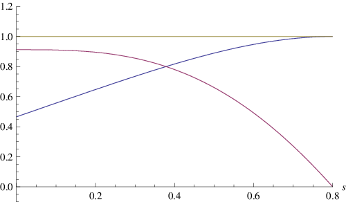
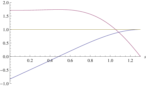
fine-tuned value of there always exists a compacton. We plot two typical compact ball
solutions in Figures 1 and 2. Here in Figure 1 starts at whereas in Figure 2 it starts at . The qualitative discussion above is completely confirmed by the numerical solutions shown in Figures 1 and 2.
4 Discussion
In this paper, we found analytic solutions for compact solitons of the shell type in 3+1 and 4+1-dimensional field theories.
To our knowledge, these are the first examples of compactons in field theories in those dimensions. The topology of these shell type compactons is quite interesting, being a combination of the topology of the complex field which lives on a compact base space ( or , respectively) and is classified by the homotopy of maps from that base space to the target space , and of the topology of the real field which lives on the positive real line (radial coordinate), and where the topology is induced by the boundary conditions implied by the finiteness of the energy. This situation is reminiscent of the Skyrme model, which has exactly the same field contents and the same topology. The main difference is the quartic kinetic term of the real scalar field in the models discussed in the present paper. Further, we were able to find an infinite number of exact compacton solutions in both cases, labelled by an integer . The existence of these infinitely many analytical solutions is probably related to the infinitely many symmetries and infinitely many conserved currents, which are present in both models, as typically happens in models with infinitely many conservation laws.
We also investigated the integrability properties of these two models and found that, although they have infinitely many conservation laws, they do not possess a generalized zero curvature representation, but a submodel defined by a further constraint equation does. In this sense, these models seem to be half way between integrable and non-integrable.
Finally we investigated a model without infinitely many symmetries, and without the scale symmetry of the models discussed above. This model does not allow for analytical solutions, but it is not difficult to find solutions numerically. It turns out that this model does not have solutions of the shell type. It does, however, possess compact solutions of the ball type, but these solutions are no longer topological solitons. The real scalar field may, in fact, take values on arbitrarily small intervals of the real axis (here is the starting value at zero radius, and 1 is the vacuum value), so the full target space may be an arbitrary segment of . Consequently, there exist compact balls with arbitrary size and energy.
As stated, it has been the main purpose of the present paper to establish the existence of compactons in field theories in higher dimensions, and to study their properties.
In the case of the shells the underlying theories are scale invariant, and
the dynamical generation of a scale (the compacton size) is by itself an important result in relativistic field theory.
Nevertheless, we want to discuss briefly some possible applications and further directions of investigation. As already mentioned, compactons in low (i.e. 1+1) dimensions have been applied to brane cosmology, where the compacton acts as a domain wall such that the confinement of both gravity and field fluctuations to the domain wall (”thick brane”) is an automatic consequence of the field equations. Recently, compact solutions of the -ball type and of the -shell type have been found in certain higher (i.e. 3+1 dimensional)
gauge theories with normal kinetic terms and V-shaped potential (for the
scalar field), [30]. Further, in Ref. [31] the coupling of these
compact balls and shells to gravity has been investigated in detail by
the use of numerical methods. It was found there that the balls may form
stable self-gravitating solutions, whereas the shells may not only form
self-gravitating shells but may also dress black holes (i.e. may contain a
Schwarzschild interior). This whole analysis is complicated by the fact that
the basic solutions of Ref. [30] are (time dependent) balls and
shells rather than static solitons (e.g. the asymptotic metric is Kerr rather
than Schwarzschild). Therefore, the coupling of the solutions of the present paper (or of related solutions of comparable simplicity) to gravity should lead to a simpler analysis of the problem of gravitational self-coupling and probably even allow for mainly analytical calculations. This question is under current investigation.
Acknowledgements
C.A., P.K. and J.S.-G. thank MCyT (Spain) and FEDER (FPA2005-01963), and support from Xunta de Galicia (grant PGIDIT06PXIB296182PR and Conselleria de Educacion). A.W. acknowledges support from the Foundation for Polish Science FNP (KOLUMB programme 2008/2009) and Ministry of Science and Higher Education of Poland grant N N202 126735 (2008-2010).
References
- [1] Arodź H 2002 Acta Phys. Polon. B 33 1241
- [2] Arodź H 2004 Acta Phys. Polon. B 35 625
- [3] Arodź H, Klimas P and Tyranowski T 2005 Acta Phys. Polon. B 36 3861
- [4] Arodź H, Klimas P and Tyranowski T 2006 Phys. Rev. E 73 046609
- [5] Klimas P 2007 Acta Phys. Polon. B 38 21
- [6] Klimas P 2008 J. Phys. A 41 095403
- [7] Arodź H, Klimas P and Tyranowski T 2008 Phys. Rev. D 77 047701, hep-th/0701148
- [8] Gaeta G, Gramchev T and Walcher S 2007 J. Phys. A 40 4493
- [9] Kuru S, arXiv:0811.0706
- [10] Adam C, Sánchez-Guillén J and Wereszczyński A 2007 J. Phys. A 40 13625
- [11] Bazeia D, Lozano L and Menezes R, 2008 Phys. Lett. B 668 246, arXiv:0807.0213
- [12] P. Rosenau and J. M. Hyman 1993 Phys. Rev. Lett. 70 564
- [13] F. Cooper, H. Shepard, P. Sodano 1993 Phys. Rev. E 48 4027
- [14] Adam C, Grandi N, Sánchez-Guillén J and Wereszczyński A 2008 J. Phys. A 41 212004
- [15] Adam C, Grandi N, Klimas P, Sánchez-Guillén J and Wereszczyński A 2008 J. Phys. A 41 375401
- [16] Bazeia D, Gomes A R, Lozano L and Menezes R 2009 Phys. Lett. B 671 402, arXiv:0808.1815
- [17] Adam C, Klimas P, Sánchez-Guillén J and Wereszczyński A, arXiv:0811.4503 [hep-th]
- [18] E. Babichev, Phys. Rev. D 74 (2006) 085004
- [19] J. Diaz-Alonso, D. Rubiera-Garcia, Annals Phys. 324 (2009) 827
- [20] De Carli E, Ferreira LA 2005 J. Math. Phys. 46 012703, hep-th/0406244
- [21] Riserio do Bonfim AC, Ferreira LA 2006 JHEP 0603:097, hep-th/0602234
- [22] Vakulenko A and Kapitansky L 1979 Sov. Phys. Doklady 24 433
- [23] Williams J G 1970 J. Math. Phys. 11 2611
- [24] Speight J M 2008 Phys. Lett. B 659 429
- [25] Adam C, Klimas P, Sánchez-Guillén J and Wereszczyński A 2009 J. Math. Phys. 50 022301, arXiv:0810.1943
- [26] Alvarez O, Ferreira L A and Sánchez-Guillén J 1998 Nucl. Phys. B 529 689
- [27] Alvarez O, Ferreira L A and Sánchez-Guillén J, arXive:0901.1654
- [28] H. Aratyn, L.A. Ferreira, and A. Zimerman 1999 Phys. Lett. B 456 162
- [29] H. Aratyn, L.A. Ferreira, and A. Zimerman 1999 Phys. Rev. Lett. 83 1723
- [30] H. Arodz, J. Lis, Phys. Rev. D 79 (2009) 045002, arXiv:0812.3284 [hep-th]
- [31] B. Kleihaus, J. Kunz, C. Lammerzahl, M. List, arXiv:0902.4799 [gr-qc]