Matrix Effective Theories of the Fractional Quantum Hall effect

Consider planar electrons of mass $m$ and electric charge $e$ in an uniform magnetic field B (in units $\hbar=1$, $c=1$). The one-particle Hamiltonian is given by:

We work in the symmetric gauge for the vector potential, $A_{i}=(\textbf{B}/2)\epsilon_{ij}x^{j},\ i,j=1,2$. The magnetic field introduces a length scale, the so-called magnetic length, $\ell=\sqrt{2/e\textbf{B}}$. The use of holomorphic spatial coordinates $z=x_{1}+ix_{2}$ and $\overline{z}=x_{1}-ix_{2}$, is natural in the QHE [15]. By introducing two commuting sets of harmonic oscillators ($\partial=\frac{\partial}{\partial z}$ and $\overline{\partial}=\frac{\partial}{\partial\overline{z}}$),

the Hamiltonian (2) and the angular momentum can be written as follows:

where $\omega=e\textbf{B}/m$ is the cyclotron frequency. Since the operators $c$ and $d$ commute, the spectrum consists of infinitely degenerate levels ($c^{\dagger}c$ excitations) with energies $\epsilon_{n}=\omega n$, i.e. the Landau levels ($d^{\dagger}d$ ladder). The degenerate states correspond to the semiclassical cyclotron orbits, that are quantized by the condition that the contained flux is a multiple of the quantum unit $\phi_{0}=eh/c$, i.e. $BA_{j}=j\phi_{0}$, with $j$ the angular momentum eigenvalue. In the lowest Landau level, the one-particle wave functions take the form:

i.e. they are holomorphic in $z$ up to an exponential factor. The associated one-particle densities are indeed peaked at the semiclassical orbits.

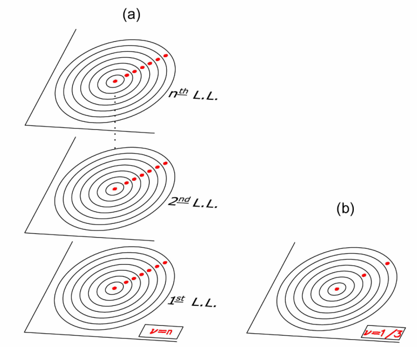
On a finite region of area $A$, the number of degenerate states is equal to the flux through the system in quantum units, $N_{\phi}={\bf B}A/\phi_{0}$. In completely filled Landau levels, the Hall conductivity is given by $\sigma_{xy}=R_{xy}^{-1}=\nu\ e^{2}/h$, where $\nu=N/N_{\phi}$ is the filling fraction, i.e. the number of electrons $N$ divided by the number of available states. Figure 2(a) shows the $\nu=n$ case in which $n$ levels are filled with one electron per orbital (the spin degree of freedom is frozen in the direction of $\bf{B}$). The density is uniform and the electron fluid is incompressible due to the exclusion principle, the gap being given by $\omega$. Thus the simple theory of free electrons in Landau levels is sufficient to describe the main physical properties of the integer QHE. (The formation of the plateaux near integer fillings is explained by the localization of excitations due to disorder) [1].

On the other hand, if there are many empty orbitals like in the case $\nu=1/3$ (Fig.2(b)), the free-electron states are compressible, in contrast with the experimental observation: the fractional QHE requires the study of interacting electrons. The formation of the gap by the Coulomb potential is clearly nonperturbative: one should try an approach based on ansatzs and effective theories, supplemented by numerical analyses. It turns out that the ground states are condensates of charges and vortices which have some analogies with superfluids and confined gauge theories, but are also specific of the two-dimensional parity breaking setting.

In a remarkable paper [3], Laughlin proposed a class of trial wave functions given by:

with $N$ the number of electrons and $m$ an integer parameter. Hereafter we set the magnetic length $\ell=1$. The wave functions (6) describe spinless electrons in the lowest Landau level: $m$ must be odd, $m=2k+1$, for antisymmetry of fermions. In order to determine the properties of these states, Laughlin used the analogy with a two-dimensional plasma, as it follows. The determination of the one-particle density can be reduced to the analysis of the two-dimensional statistical model of charges defined by,

In this equation, $H_{plasma}$ describes a classical plasma of charges in a uniform background at temperature $\beta=1/m$. Knowing that this plasma is totally screened for small values of $m$, Laughlin could argue that the density is uniform and could calculate the gap of excitations. For constant density, the parameter $m$ can be readily related to the filling fraction by $\nu=1/m$. Note that Laughlin’s wavefunctions vanishes as $\left(z_{i}-z_{j}\right)^{m}$ when any two particles $i$ and $j$ approach each other: namely, the amplitude for nearby particles is very small and the expectation value of the Coulomb energy is consequently reduced. This is a rather successful property from the variational point of view, since other wave functions with same average density do have this feature. Numerical experiments show that the Laughlin wavefunction is actually very close to the exact ground state for several short-range repulsive interactions [1][3][16].

Laughlin also proposed the wave functions of the low-energy quasiholes excitations: they are localized density deformations,

with $\eta$ the position of the vortex (Fig.3). To calculate the charge of the quasi-hole, one can use the plasma analogy (7):

Comparing (9) with (7), we observe that the electrons feel the presence of a charge $1/m$ at the point $z=\eta$: thus, the quasi-holes have fractional charge $Q_{qh}=e/m$ [3].

In the wave function for two quasi-holes,

Laughlin introduced the term $(\eta_{1}-\eta_{2})$ raised to a fractional power, that is necessary for charge equilibration in the plasma (9); he assumed a holomorphic dependence as for the electron coordinates [17]. If we rotate one quasi-hole around the other, we obtain:

Therefore, the wave function acquires a non-trivial phase under exchanges of excitations: the quasi-holes have “fractional statistics”, $\frac{\theta}{\pi}=\frac{1}{2k+1}$. This is a long-range, topological interaction of vortices, that is allowed in parity breaking two-dimensional systems [17]. The fractional charge and statistics of excitations are confirmed by the effective field theory descriptions to be discussed later. The fractional charge has been observed in experiments of quasiparticle tunneling [4]; the fractional statistic has not been detected directly but there are indirect confirmations [1].

In Fig. 1, one finds stable plateaux at other filling fractions that are nicely accounted by the series $\nu=n/(2nk\pm 1)$ with $n>1$. The phenomenological theory due to Jain explains them as follows: the argument starts by observing that the inverse filling,

is equal the number of fluxes per electron. Imagine that it is possible to bound an even number of fluxes, i.e. $2k$, to each electron, to form a new quasiparticle called “composite fermion”. (Note that an even number of flux quanta yield an integer Aharonov-Bohm phase and keeps the fermionic statistics). When $2k$ fluxes are attached to each electron, the same number of fluxes are removed from the external magnetic field: therefore, the filling fraction of the system of composite fermions is given by

corresponding to an integer QHE. The reduced magnetic field felt by the new particles is given by $\textbf{B}^{\star}$. This is indeed observed: many experiments confirm the existence of weakly interacting excitations feeling the reduced magnetic field, i.e. behaving as Jain’s composite fermions [1]. The incompressibility of the fractional QHE is explained by Jain as due to the equivalence between the system of electrons with $\nu=n/(2nk+1)$ and the integer QHE of composite fermions with $\nu^{\star}=n$.

Following the Jain argument, the flux attachment is clear in the form of the Laughlin wave function ($\nu^{\star}=1$): the factor $\Pi^{N}_{i<j}(z_{i}-z_{j})^{2k}$ yields Aharonov-Bohm phase of $2k$ flux quanta to any electron, and the rest is the wave function of the filled first Landau level. In the general case of $\nu=n/(2nk+1)$, the ground state wave functions proposed by Jain on the basis of his equivalence are:

with $\Psi_{1/n}(z_{1},...,z_{N})$ being the wave functions with $n$ completely filled levels (Slater determinants). The Jain wave functions (14) have been confirmed by comparison with numerical results of exact diagonalization of the Hamiltonian with Coulomb interaction [5]. The fillings $\nu=n/(2nk-1)$ are also described by (14) with charge-conjugate term $\Psi_{1/n}\to\overline{\Psi}_{1/n}$.

The Jain scheme also provide excellent approximations for the quasi-holes and quasi-particles excitations [5]. For instance, a quasi-particle in the origin for the Jain state with $\nu=n/(2nk+1)$ is given by,

where $\Psi_{qp;1/n}(z_{1},...,z_{N})$ corresponds to the wave function of $n$ filled Landau levels and one electron in the first orbital of the $(n+1)$-th Landau level. The corresponding localized density has an excess of charge at the origin of the droplet.

Among the effective field theories that have been proposed to describe the fractional QHE, we recall the theory of non-relativistic fermions coupled to the Abelian Chern-Simons “statistical” interaction, that has been developed by Fradkin and Lopez [6] and others [7]. The action can be schematically written:

Consider the Gauss law of this theory:

where $\mathcal{B}$ is the “statistical” magnetic field and $\kappa$ the Chern-Simons coupling constant. At quantum level, this is an operator constraint which selects the physical space of states. These are charge-flux composites: every particle with unit electric charge carries a magnetic charge equal to $2\pi/\kappa$. The wave functions for these composite particles exhibits Aharonov-Bohm effects changing the statistics. Therefore a fermion coupled to a Chern-Simons gauge field behaves like an anyon with statistical angle $\theta/\pi=1/\kappa$, measured with respect to the Fermi statistics [6]. If $\kappa=1/2k$, where $k$ is an integer, then $\theta/\pi=2k$ and the composite states are still fermions.

A ground state with uniform density $\langle j_{0}(z)\rangle=\bar{\rho}$ implies a constant field:

Eq. (18) shows that, within the mean field approximation, the effect of the statistical gauge field is to change the effective flux experienced by the fermionic excitations. The effective magnetic field is $B_{eff}=\textbf{B}+\langle\mathcal{B}\rangle=\textbf{B}-2\kappa 2\pi\rho_{0}$, in agreement with Jain’s argument (13).

The uniform effective magnetic field $B_{eff}$ defines a new set of effective Landau levels. Each level has a degeneracy equal to the total number of effective flux quanta $N_{eff}$ and the separation between levels is the effective cyclotron frequency $\omega_{eff}=|B_{eff}|/m$. Similarly, there is an effective cyclotron radius $\ell_{eff}$. It is easy to see that the mean-field approximation (uniform density) (18) is selfconsistent only if the fermions fill exactly an integer number $n$ of effective Landau levels. This reproduces Jain’s theory: the fractional QHE is the integer QHE of a system of electrons dressed by an even number of flux quanta. The allowed filling fractions are those obtained by Jain: $\nu=n/(2nk\pm 1)$ [6]. Further results of this approach are reviewed in [18].

Let us mention for completeness the effective field theory approaches based on $(1+1)$ dimensional conformal field theories. As originally observed by Wen [19], a droplet of incompressible fluid possess low-energy massless chiral excitations at the edge, that can be described by conformal field theories with $U(1)$ current, also called chiral Luttinger liquid theories, and their generalizations. These theories of the QHE have been extensively developed in the last 20 years and can describe the low-energy physics occurring in conduction experiments [1] [19] [20]. In this approach, the formation of the incompressible fluid is assumed and cannot be derived, since the dimensional reduction is only possible for these specific states; actually, there is a different conformal field theory for each plateaux, whose form can be inferred by the properties of excitations and other data. In the following, we deal with $(2+1)$-dimensional effective theories that could explain the formation of incompressible ground states.

Every noncommutative theory is equivalent to a matrix theory, with matrices of infinite order ($N\to\infty$) [24]; in particular, the noncommutative Chern-Simons theory (27) is equivalent to the matrix theory [25]:

where now $X_{1}(t),X_{2}(t)$ and $A_{0}(t)$ are $N\times N$ matrices ($N\rightarrow\infty$) and the covariant derivative is $D_{t}X_{j}=\dot{X_{j}}-i\left[A_{0},X_{j}\right]$ , $j=1,2$.

The proof of the correspondence is simpler if we go from the matrix (30) to the noncommutative theory (27). Observe that the Gauss law of the Lagrangian (30) implies the following noncommutative condition on the matrices:

with $I$ the identity matrix. This algebra only admits $\infty$-dimensional matrix representations: consider a particular, “ground state” solution, $X=\hat{x}^{i}$, and write the general solutions as follows:

where $A_{i}$ are $N\times N$ matrices of “fluctuations” ($N\rightarrow\infty$). Note that these matrices can be expressed in terms of finite sums of products $e^{ip\hat{x}^{1}}e^{iq\hat{x}^{2}}$, i.e. they can be thought of being functions of $\hat{x}^{i}$. Replacing (32) in (30) and expressing the derivative as commutators, $\left[\hat{x}^{i},f(\hat{x}^{1},\hat{x}^{2})\right]=i\theta\epsilon^{ij}\partial_{j}f$, we find:

or in covariant notation,

In the limit $N\rightarrow\infty$ the matrix variables $A_{i}$ are mapped into smooth functions of the noncommutative coordinates $A_{i}(\hat{x}_{j})$. Also in this limit we can identify, $\theta{\rm Tr}\rightarrow\frac{1}{2\pi}\int d\hat{x}_{1}d\hat{x}_{2}$, and we obtain the following Lagrangian:

In this Lagrangian, the fields $A_{i}$ still obey the matrix algebra, while in (27) they are functions. The two formulations are related by expressing matrices as Wigner $c$-number functions that obey the Moyal product algebra [15].

Let us recall that any operator $\hat{F}(\hat{x_{1}},\hat{x_{2}})$ in the Weyl ordering $:\ :$ (most symmetric in $\hat{x_{1}},\hat{x_{2}}$) can be associated to a phase space function $F(x_{1},x_{2})$ as follows:

One finds by inspection that the product of two operators $\hat{F}$ and $\hat{G}$ corresponds to the Moyal product (28) of the corresponding Wigner functions, $:\hat{F}:\ :\hat{G}:=:\hat{H}:$, $H(x_{1},x_{2})=(F\star G)(x_{1},x_{2})$. In particular,

Therefore, the matrix Lagrangian (35) becomes the noncommutative Chern-Simons theory (27) (within the Weyl ordering).

Finally, we recall that another route to obtain the Chern-Simons matrix theory (30), that emphasizes the discrete particle aspects of the fluid is given by a matrix regularization proposed by Goldstone and Hoppe [26].

The noncommutative Chern-Simons Lagrangian (27) and its matrix model formulation (30) both imply infinite degrees of freedom: therefore, Susskind’s theory applies to an infinite system. Instead, the fractional QHE is a system with a boundary and a finite number of particles. Polychronakos introduced this feature [9] by modifying Susskind’s action (30) as follows:

Two new terms are present: the first is a quadratic potential that confines the eigenvalues, i.e. keep the particles localized in the plane, with $\sigma=O(\textbf{B}/N)$; the second term is a “boundary” $N$-dimensional complex vector $\psi$ that transforms in the fundamental representation of the gauge group $U(N)$. The Gauss law is now given by:

Observe that the trace of (39) implies,

that can be realized with $N\times N$ dimensional matrices. The action (38) thus defines the Chern-Simons matrix model, a gauge theory with $U(N)$ symmetry, $X_{a}\rightarrow UX_{a}U^{\dagger}$, $\psi\rightarrow U\psi$ and $A_{0}\rightarrow UA_{0}U^{\dagger}-iU\frac{dU^{\dagger}}{dt}$. Under a gauge transformation the action (38) is not invariant, but it yields a winding number, $S\rightarrow S-i\textbf{B}\theta\int dtTr\left[U^{\dagger}\dot{U}\right]$; this requires the quantization $\textbf{B}\theta=k$ [27], leading to the Laughlin filling fractions (cf.(26)). Note that the equation of motion for $\psi$ in the $A_{0}=0$ gauge read, $\dot{\psi}=0$, showing that this is an auxiliary field with trivial dynamics; it can take the constant value $\psi=\sqrt{N\textbf{B}\theta}\mid v\rangle$, with $\mid v\rangle$ a vector of unit length [9].

In the $A_{0}=0$ gauge, the Hamiltonian of the Polychronakos theory (38) corresponds to $(N^{2}+N)$ particles in the lowest Landau level with coordinates $X_{nm}$ and $\psi_{n}$. It can be shown that, at quantum level, the Gauss law (39) implies gauge invariant states of the form $\Psi(X,\psi)=e^{-Tr(\bar{X}X)/2-\psi^{\dagger}\psi/2}\Phi(X,\psi)$, with $\Phi(X,\psi)$ a singlet of the gauge group $U(N)$ made by polynomials of $X_{nm}$ and $\psi_{n}$, being of order $Nk$ in $\psi_{n}$ due to (40) [10]. A basis of states is given by:

These states are eigenstates of the angular momentum $J$ with eigenvalues ${\cal J}=N_{X}$, where $N_{X}$ is the number of matrices $X$ appearing in $\Phi(X,\psi)$. Since the Hamiltonian of the theory is proportional to the angular momentum, $H=(2\omega/{\bf B})\ J$, the states (41) are also eigenstates of the Hamiltonian. The ground state of the theory is [10]:

corresponding to the lowest value of the angular momentum (lower order polynomials vanish by antisymmetry of the $\epsilon^{i_{1}...i_{N}}$ tensor).

If we now diagonalize the matrix $X$ by the similarity transformation, $X=V^{-1}\Lambda V$, with $\Lambda=diag(\lambda_{1},\dots,\lambda_{N})$, we obtain:

The quantity $C$ appears in all the physical states and can be neglected in the present discussion [11].

Therefore we have obtained the Laughlin wave function as the ground state of the Chern-Simons theory, with electron coordinates identified with the eigenvalues of $X$. This is a very important result of the Chern-Simons matrix theory; that of reproducing the Laughlin wave function from gauge invariance of the states in presence of the “background charge” $\theta$. (Note that the filling fraction is $\nu=1/(k+1)$: the shift from the classical value (26) is due to a Vandermonde factor coming from the integration measure [9]).

Let us now discuss the excitations over the ground state (42). In Ref.[10], it was found the “bosonic” basis of states,

for any positive integers $\{m_{1},\dots,m_{k}\}$. These states have $\Delta{\cal J}=r=\sum_{k}m_{k}$. For $r=O(1)$, their energy given by the boundary potential, $\Delta E=\sigma\Delta{\cal J}=O(r\ {\bf B}/N)$ is very small: they are the edge excitations of the droplet of fluid described by conformal field theories [15][19][20].

The matrix model also possess localized density deformations that are analogues of the quasi-hole excitations of the Laughlin state. For example, the state $\Phi_{\{n_{1},\dots,n_{N}\}}$ in Eq.(41), with $\{n_{1},n_{2},\cdots,n_{M}\}=\{1,2,\cdots,N\}$, corresponds to moving one electron from the interior of the Fermi surface to the edge, causing $\Delta{\cal J}=O(N)$ and thus a finite gap $\Delta E=O({\bf B})$. On the other hand, the quasi-particle excitation cannot be realized in the Chern-Simons matrix model [9][12][14], because excitations with angular momentum lower than (42) are zero due to the antisymmetry of the $\epsilon^{i_{1}...i_{N}}$ tensor. Similarly, the Jain states $\nu=n/(2nk+1)$ are not naturally obtained [28].

In conclusion, we have shown that the Chern-Simons matrix model reproduces the Laughlin wave functions as ground states. Nevertheless, the theory has some drawbacks [13]: there are no quasi-particle excitations [9], and the Jain states cannot be described [28]. Moreover, the measure of integration w.r.t. the eigenvalues $\lambda_{i}$ differs from that of electrons in the lowest Landau level, owing to the noncommutativity of matrices. It can be shown that the ground state properties of the matrix theory and of the Laughlin state only agree at long distances [11][29]. Owing to the inherent noncommutativity, it is also difficult to match matrix observables with electron quantities of the quantum Hall effect [30].

We would like to stress that the Chern-Simon matrix model provides another realization of the Jain composite-fermion transformation (see section 2.3). For $k=0$, the matrix theory reduced to the eigenvalues $\lambda_{a}$ is equivalent to a system of free fermions in the lowest Landau level, i.e. to $\nu^{*}=1$ [11][29]. This fermionic picture is a general feature of one-dimensional matrix models [31].

In the presence of the $\theta$ background, the noncommutativity of matrix coordinates (39) forces the electrons to acquire a finite area of order $\theta$, leading to the (semiclassical) density $\rho_{o}=1/2\pi\theta$ (23). Using this formula of the density and the quantization of ${\bf B}\theta$, we re-obtain the Jain relation (13) for flux attachment,

Given that noncommutativity is expressed by the Gauss law of the matrix theory, we understand that the mechanism for realizing the Jain transformation is analogous to that of the Lopez-Fradkin theory (cf. (18), section 2.4), but it is expressed in terms of different variables. However, the higher Landau levels are not possible in the Chern-Simons matrix model.

Let us briefly review Witten’s derivation of the effective low-energy action of $N$ Dp-branes [34]. Consider ten-dimensional Minkowski space, with time $x^{0}$ and space $x^{1},...,x^{9}$ coordinates, respectively. A p-brane is an object that modifies the boundary conditions of open strings: it introduces Dirichlet boundary conditions in $(9-p)$ directions, as follows,

Due to (47), the zero modes $X^{j}$ with $j>p$ are frozen, and the massless particles are functions of $X_{1},..,X_{p}$ only. The massless bosons $A_{i}(X^{s})$, $i,s=0,...,p$, propagate as $U(1)$ gauge bosons on the p-brane, while the other components become scalars fields on the p-brane, $\phi_{j}(X^{s})$, $j>p$. The vertex operators for insertions of spin-$1$ fields in string theory are given by:

For $\phi_{j}=$constant, the boundary integral of $V_{\phi}$ implies the change $X^{j}\rightarrow X^{j}+\phi^{j}$ for $j>p$: thus the scalars $\phi_{j},j>p$ can be interpreted as the coordinates of the p-brane. The theory on the $(p+1)$ dimensional brane world-volume is naturally the ten-dimensional $U(1)$ supersymmetric gauge theory dimensionally reduced to $(p+1)$ dimensions.

Bound states of $N$ parallel Dirichlet p-branes can be described by the low-energy limit when the branes are nearby. We consider the case of two parallel Dirichlet p-branes, one at $X^{j}=0$, and one at $X^{j}=a^{j}$ ($j>p$). The branes are connected by strings: they can start and end on the same brane and give a $U(1)\times U(1)$ gauge theory (with one $U(1)$ living one each p-brane), or they can start in the first brane and end in the second (and viceversa). In this case, the strings have $U(1)\times U(1)$ charges. The ground state of this configuration has an energy $T\mid a\mid$, with $T$ and $\mid a\mid$ being the tension and length of the string, respectively. When $\mid a\mid\rightarrow 0$ the charged vector bosons become massless and the $U(1)\times U(1)$ gauge symmetry is enlarged to a $U(2)$ symmetry. In the same way, $N$ coincident parallel branes yield a $U(N)$ gauge symmetry on the p-brane. The field content in the effective action is given by the $U(N)$ gauge field $A_{j}(X^{s},t)$, with $s,j=1,...,p$ , and the scalar fields $\phi_{j}(X^{s},t)$, with$j>p$ , in the adjoint representation of $U(N)$, i.e. they are all $N\times N$ matrices.

The reduction to $(p+1)$ dimensions of the bosonic sector of the theory is obtained as follows. From the Lagrangian,

we simplify the commutators in $F^{\mu\nu}=\left[D_{\mu},D_{\nu}\right]$ by dimensional reduction and identify the earlier fields, leading to:

References

- [1] For a review see: R. A. Prange and S. M. Girvin, The Quantum Hall Effect, Springer, Berlin (1990); S. Das Sarma and A. Pinczuk, Perspectives in Quantum Hall effects, Wiley, New York (1997).
- [2] D. Tsui, H. Sormer, A .Gossard, Two-Dimensional Magnetotransport in the Extreme Quantum Limit, Phys. Rev. Lett. 48 (1982) 1559.
- [3] R. B. Laughlin, Anomalous Quantum Hall Effect: An Incompressible Quantum Fluid with Fractionally Charged Excitations, Phys. Rev. Lett. 50 (1983) 1395; Elementary Theory: the Incompressible Quantum Fluid, in R. A. Prange and S. M. Girvin, Ref. [1].
- [4] L. Saminadayar, D. C. Glattli, Y. Jin, and B. Etienne, Observation of the e/3 Fractionally Charged Laughlin Quasiparticle, Phys. Rev. Lett. 79 (1997) 2526; R. de-Picciotto, M. Reznikov, M. Heiblum, V. Umansky, G. Bunin and D. Mahalu, Direct observation of a fractional charge, Nature 389 (1997) 162.
- [5] J. Jain, Composite Fermions, Cambridge Univ. Press, Cambridge (2007).
- [6] A. Lopez, E. Fradkin, Fractional Quantum Hall Effect and Chern-Simons gauge theories, Phys. Rev. B 44 (1991) 5246; Universal properties of the wave functions of fractional quantum Hall systems, Phys. Rev. Lett. 69 (1992) 2126.
- [7] S. Kivelson, D.-H. Lee, and S.-C. Zhang, Global phase diagram in the quantum Hall effect, Phys. Rev. B 46 (1992) 2223; S. C. Zhang, The Chern-Simons-Landau-Ginzburg theory of the fractional quantum Hall effect, Int. J. Mod. Phys. B 6 (1992) 25; G. Murthy, R. Shankar, Hamiltonian Theories of the FQHE, Rev. Mod. Phys.75 (2003) 1101.
- [8] L. Susskind, The quantum Hall fluid and non-commutative Chern Simons theory, hep-th/0101029.
- [9] A. P. Polychronakos, Quantum Hall states as matrix Chern-Simons theory, JHEP 0104 (2001) 011; Quantum Hall states on the cylinder as unitary matrix Chern-Simons theory, JHEP 0106 (2001) 070.
- [10] S. Hellerman and M. Van Raamsdonk, Quantum Hall physics equals noncommutative field theory, JHEP 0110 (2001) 039.
- [11] A. Cappelli and M. Riccardi, Matrix model description of Laughlin Hall states, J. Stat. Mech. 0505 (2005) P001.
- [12] A. Cappelli and I. D. Rodriguez, Jain states in a matrix theory of the quantum Hall effect, JHEP 0612 (2006) 056.
- [13] T. H. Hansson, J. Kailasvuori, A. Karlhede and R. von Unge, Solitons and Quasielectrons in the Quantum Hall Matrix Model, Phys. Rev. B 72 (2005) 205317.
- [14] A. Cappelli and I. D. Rodriguez, Semiclassical Droplet States in Matrix Quantum Hall Effect, JHEP 0802 (2008) 046.
- [15] A. Cappelli, C. A. Trugenberger and G. R. Zemba, Infinite symmetry in the quantum Hall effect, Nucl. Phys. B 396 (1993) 465; Large N limit in the quantum Hall Effect, Phys. Lett. B 306 (1993) 100; for a review, see: Nucl. Phys. B (Proc. Suppl.)33C (1993) 21.
- [16] F. D. M. Haldane, The hierarchy of fractional states and numerical studies, in R. A. Prange and S. M. Girvin [1]; J. Jain et al., in [5]; A. Cappelli, C. Méndez, J. Simonin, G. R. Zemba, Numerical study of hierarchical quantum Hall edge states on the disk geometry, Phys. Rev. B 58 (1998) 16291;
- [17] F. Wilczek, Fractional Statistics and Anyon Superconductivity, World Scientific, Singapore (1990).
- [18] A. Lopez, E. Fradkin, Fermionic Chern-Simons Field Theory for the Fractional Hall Effect, in Composite Fermions: A Unified View of the Quantum Hall Regime, O. Heinonen Ed., World Scientific, Singapore (1998).
- [19] X.-G. Wen, Quantum Field Theory of Many-Body Systems, Oxford Univ. Press, Oxford (2004).
- [20] J. Fröhlich and A. Zee, Large scale physics of the quantum Hall fluid, Nucl. Phys. B 364 (1991) 517; X.-G. Wen and A. Zee, Classification of Abelian quantum Hall states and matrix formulation of topological fluids, Phys. Rev. B 46 (1993) 2290; A. Cappelli, C. A. Trugenberger and G. R. Zemba, Classification of quantum Hall universality classes by W(1+infinity) symmetry, Phys. Rev. Lett. 72 (1994) 1902; Stable hierarchical quantum hall fluids as W(1+infinity) minimal models, Nucl. Phys. B 448 (1995) 470.
- [21] J. H. Brodie, L. Susskind and N. Toumbas, How Bob Laughlin tamed the giant graviton from Taub-NUT space, JHEP 0102 (2001) 003; B. Freivogel, L. Susskind and N. Toumbas, A two fluid description of the quantum Hall soliton, hep-th/0108076; O. Bergman, Y. Okawa and J. H. Brodie, The stringy quantum Hall fluid, JHEP 0111 (2001) 019; A. Ghodsi, A. E. Mosaffa, O. Saremi and M. M. Sheikh-Jabbari, LLL vs. LLM: Half BPS sector of N = 4 SYM equals to quantum Hall system, Nucl. Phys. B 729 (2005) 467; J. Dai, X. J. Wang and Y. S. Wu, Dynamics of giant-gravitons in the LLM geometry and the fractional quantum Hall effect, Nucl. Phys. B 731 (2005) 285.
- [22] G. V. Dunne, R. Jackiw and C. A. Trugenberger, ’Topological’ (Chern-Simons) Quantum Mechanics, Phys. Rev. D 41 (1990) 661.
- [23] R. Jackiw, S. Y. Pi and A. P. Polychronakos, Noncommuting gauge fields as a Lagrange fluid, Ann. Phys. (NY) 301 (2002) 157; R. Jackiw, A. P. Polychronakos, Perfect fluid theory and its extensions, J. Phys. A 37 327 (2004); A. P. Polychronakos, Noncommutative Fluids, arXiv:0706.1095, to appear in Seminaire Poincare X, IHP, Paris.
- [24] N. Seiberg and E. Witten, String theory and noncommutative geometry, JHEP 9909 (1999) 032; M. R. Douglas and N. A. Nekrasov, Noncommutative field theory, Rev. Mod. Phys. 73 (2001) 977.
- [25] N. Seiberg, A note on background independence in noncommutative gauge theories, matrix model and tachyon condensation, JHEP 0009 (2000) 003; J. H. Brodie, L. Susskind and N. Toumbas, in [21].
- [26] J. Hoppe, Ph.D. thesis (Massachusetts Institute of Technology), (1982).
- [27] V. P. Nair and A. P. Polychronakos, On level quantization for the noncommutative Chern-Simons theory, Phys. Rev. Lett. 87 (2001) 030403.
- [28] B. Morariu and A. P. Polychronakos, Finite noncommutative Chern-Simons with a Wilson line and the quantum Hall effect, JHEP 0107 (2001) 006.
- [29] D. Karabali and B. Sakita, Orthogonal basis for the energy eigenfunctions of the Chern-Simons matrix model, Phys. Rev. B 65 (2002) 075304; Chern-Simons matrix model: Coherent states and relation to Laughlin wavefunctions, Phys. Rev. B 64 (2001) 245316.
- [30] T. H. Hansson and A. Karlhede, Charges and Currents in the Noncommutative Chern-Simons Theory of the QHE, cond-mat/0109413; T. H. Hansson, J. Kailasvuori and A. Karlhede, Charge and Current in the Quantum Hall Matrix Model, Phys. Rev. B 68, 035327 (2003).
- [31] E. Brezin, C. Itzykson, G. Parisi and J. B. Zuber, Planar Diagrams, Commun. Math. Phys. 59 (1978) 35; M.L. Mehta, Random Matrices and the statistical theory of energy levels, Academic Press, New York (1967).
- [32] J. A. Harvey, Komaba lectures on noncommutative solitons and D-branes, [hep-th/0102076]; J. Polchinski, String Theory, Vol.2 Cambridge Univ. Press, Cambridge (1998).
- [33] T. Banks, W. Fischler, S. H. Shenker and L. Susskind, M theory as a matrix model: A conjecture, Phys. Rev. D 55 (1997) 5112; W. Taylor, M(atrix) theory: Matrix quantum mechanics as a fundamental theory, Rev. Mod. Phys. 73 (2001) 419.
- [34] E. Witten, Bound states of strings and p-branes, Nucl. Phys. B 460 (1996) 335.
- [35] J. H. Park, On a matrix model of level structure, Class. Quant. Grav. 19 (2002) L11.
- [36] V. Pasquier, F.D.M. Haldane, A dipole interpretation of the state, Nucl. Phys. B (FS) 516 (1998) 719; V. Pasquier, Skyrmions in the quantum Hall effect and noncommutative solitons, Phys. Lett. B 490 (2000) 258.
- [37] J. Lambert and M. B. Paranjape, Quasi-hole solutions in finite noncommutative Maxwell-Chern-Simons theory, JHEP 0705 (2007) 007.
- [38] A. P. Polychronakos, Multidimensional Calogero systems from matrix models, Phys. Lett. B 408 (1997) 117.
- [39] A. P. Polychronakos, Physics and mathematics of Calogero particles, J. Phys. A 39 (2006) 12793.
- [40] D. C. Cabra, N. E. Grandi, Incidence of the boundary shape in the effective theory of fractional quantum Hall edges, Phys. Rev. B 77 (2008) 115107; I. D. Rodriguez, Edge excitations of the Chern Simons matrix theory for the FQHE, arXiv:0812.4531.
- [41] A. Cappelli and G. R. Zemba, Hamiltonian formulation of the W(1+infinity) minimal models, Nucl. Phys. B 540 (1999) 610; D. Orgad and O. Agam, Correlated Tunneling and the Instability of the Fractional Quantum Hall Edge Phys. Rev. Lett. 100 (2008) 156802.