Numerical studies on the self-similar collapse of the -patches problem
Abstract
This paper studies the dynamical evolution of the patches problem expressed in self-similar variables. A numerical algorithm is proposed and these equations are numerically explored. Several benchmarks of the code are discussed throughout the paper. Exact self-similar solutions are described and are found to play a role in separating collapsing from non-collapsing initial data: small perturbations around this solution blow up while others do not. Numerical simulations performed near convergent rescaled profiles, such as those described by Córdoba et al. in [pnas], indicate the absence of a stationary graph in the neighborhood of the rescaled profiles and suggest a more complex scenario for blow up.
Mathematics Subject Classification: 65M99, 35Q35
1 Introduction
A classical open problem in mathematical fluid mechanics is whether 3D Euler equations may develop singularities in finite time [Const]. One of the scenarios proposed in the past for the formation of singularities in Euler equations is the vortex patch problem. A vortex patch consists of a 2D simply connected and bounded region of constant vorticity which is a weak solution of the 2D Euler equation. The work of Chemin [Che] and Bertozzi and Constantin [BeCo] rigorously proved the global existence of regular solutions for this case, and therefore in the context of this equation singularities cannot appear.
The 2D surface quasigeostrophic equations have also attracted a lot of interest mainly because of their similarity to the 3D Euler equations [CMT] and its physical relevance as a model for the formation of temperature fronts in some geophysical contexts [CMTpof, CMT, CFR, Ped]. They model a two-dimensional incompressible fluid system, and since it is a 2D model it is more tractable than the full 3D Euler system. A very actively studied question for this system is the formation of singularities in finite time for smooth initial data (see [jap, diego, cf, dh, ccw, clstw]).
The -patches problem is a family of contour dynamics equations that links the vortex patches scenario to the evolution of patches in the surface quasi-geostrophic equation. This problem has been analyzed by Córdoba et al [pnas]. In this setting, the time evolution of a point, , in any of the contours that surrounds a patch with constant is described by the equation,
| (1) |
Here the sum extends up to , the number of patches. The integrals along the contours are done counterclockwise. This is a family of equations depending on the parameter . In the limit the equation approaches the vortex patch problem of the 2D Euler equation whereas the limit approaches the surface quasi-geostrophic equation.
The solutions of the -patches problem are numerically explored in the range by Córdoba et al. [pnas] for the case of two patches and evidence of collapse is reported. Numerical evidence of blow up is a disputable issue, since numerical calculations supporting this evidence do not constitute a formal proof. This was the case, for instance, for the 2D Euler equation [Bu, DM] and still is for the 3D Euler equation [kerr]. The current article completes the results by Córdoba et al. describing in detail the numerical method used to perform the simulations and providing benchmarks for this method. Additionally the numerical results by Córdoba et al. provide evidence that in the -patches problem, subsequent to a self-similar rescaling involving the parameter , the collapsing curves converge towards a unique profile, thus suggesting the existence of a fixed point for the self-similar problem. While this problem was proposed in [pnas], it was not thoroughly studied there. The current article is also focused in the study of collapse for , particularly for the selection , but makes progress by extending the numerical simulations to the problem reformulated in self-similar variables. The advantage of using rescaled variables is that the finite time collapse observed by Córdoba et al., becomes an asymptotic limit in the pseudo-time , and thus the evolution may be more accurately described. Our findings rule out the presence of a stationary graph for the self-similar equation close to the convergent rescaled profiles. However, a different but exact fixed point is described, which is found to play a role in separating collapsing from non-collapsing initial data.
This article is organized as follows: Section 2 describes the problem; in particular the equations under study are introduced and the derivation of the self-similar equations is explained. General blow up conditions are deduced for this setting. Section 3 reports on the numerical methods employed in the simulations. Section 4 provides an account of the results. Finally, the conclusions are presented in Section 5.
2 The equations
In accordance with Zabusky et al. [Z] the velocity of a particle on the contour of a patch for the 2D vortex patch problem is obtained by inverting the relation between the streamfunction and the vorticity. For the -patches problem this relation is generalized by , where is the streamfunction and is the scalar that takes a constant value within the patch. In the limit , which corresponds to the 2D Euler equation, the scalar plays the role of vorticity and in the limit (the quasi-geostrophic equation) the scalar corresponds to the potential temperature. For one obtains that the velocity of a particle on the contour is given by:
| (2) |
Here denotes the position of a particle on the contour . This contour is parametrized by , and in our convention the integral along it is done counterclockwise. Here , where the factor results from inverting the operator and is the value of scalar in the patch. Changing the sign in the value of is equivalent to reversing the circulation along the integral in our convention.
The contour dynamic equation is eventually obtained by replacing the velocity of a particle by the time derivative of its trajectory, i.e.:
This article focuses on the contour evolution of two patches. The time evolution of a point in any of the contours is described by the equation:
| (3) |
In the limit , which is the case of the quasigeostrophic equation, local existence has been reported in [Ro, paco]. In this case one should use (see [Ro]) the following formula for the velocity (in the one-patch case):
| (4) |
This equation eliminates the tangential component of the velocity, as only the normal component is able to deform the curve, thereby avoiding divergent integrals.


Simulations reported in [pnas] on Eq. (3) for show evidence of self-similar collapse. Figure 1 illustrates the collapse for of two ellipses with semi-axis 1.1 (along the horizontal direction) and 1 (along the vertical coordinate) centered at positions and , on which and the integrals are counterclockwise circulating. The singularity is point-like as shown in the magnification of Fig. 1(a) for a sequence near the corner. This result is consistent with the absence of splash singularity proven for this problem by Gancedo and Strain [paco2], as it is found that the curvature also blows up. The coordinates of the collapse point are denoted as , where is the collapse time. Numerical results reported in [pnas] indicate that scaling laws exist near the blow up that describe the evolution of the maximum curvature as:
| (5) |
and also describe the minimum distance between contours as:
| (6) |
Fig. 1(b) shows the profiles displayed in Fig. 1(a) after rescaling by a factor and adjusting the output conveniently to achieve the coincidence in a independent pattern.
The result displayed in Fig. 1(b) led Córdoba et al. [pnas] to propose an equation for the rescaled spatial variable :
| (7) |
where , and the velocity of the scaling function is given by
The equation of motion for the rescaled space variable is:
| (8) |
where are the rescaled contours. The new time variable
| (9) |
transforms the equation (8) into the self-similar equation:
| (10) |
Like the non-rescaled equation, this equation admits a projection over , the unitary normal component to the curve at , which is useful for describing the case,
| (11) |
The projection evolves in time the same as the system (10) , since only the normal component deforms the curve. The rescaled contours shown in Fig. 1(b), which seem to coincide over a unique curve, suggest that Eq. (11) has a fixed point, also called a self-similar solution. Should an attracting fixed point linked to this pattern be found, it would be of great interest as it would provide a path toward rigorous proof for the existence of blow up. We will examine this possibility further in the results section.
Interesting relations exist between the original and rescaled variables. For instance, the blow up in the original variables is transformed into an asymptotic behavior in the self-similar variables. In this way, the collapse reported in [pnas], which occurs in a very small time interval in original variables, is mapped to an infinite interval in rescaled variables, thus permitting a detailed monitoring of the blow up. We now consider the area of the patches; this is related to the energy of the initial data and is conserved in the original variables . However, according to Eq. (7), it tends to grow in the rescaled variables . Other connections between the rescaled and non-rescaled variables concern distance. The shortest distance, , between collapsing contours (see Eq. (6) and Fig. 1(a)) tends to zero in the original variables, but is not necessarily zero in the new variables (see Fig. 1(b)). These results are easily justified. Since collapse is point-like, the distance between contours at the blow up time becomes zero just for two trajectories, one on each contour, thus satisfying,
| (12) |
The distance between these trajectories in self-similar variables is given by,
| (13) |
The factor in Eq. (13) confirms that the null distance between the original variables is satisfied even if trajectories on the rescaled variables are at a finite distance above zero at the collapse time . The above expression may be rewritten in terms of the pseudo-time , as follows:
| (14) |
As explained in the following section, the numerical technique used for simulations does not track individual particles on contours, but rather the contour as a whole, so the above collapse trajectories are not numerically integrated, only the contour that contains them. It is expected that near the collapse, the distance between these trajectories will be well represented by the evolution of the shortest distance between contours which in [pnas] is reported to evolve according to the expression:
| (15) |
Here represents the set of points on the contours that are at a shortest distance as a function of time and is a constant. Similarly, the collapse may be also tracked in the self-similar variables as the shortest distance between contours. This distance in the self-similar variables is related to that in the non self-similar variables by the expression:
| (16) |
Let us define the minimum distance between contours in the self-similar variables as:
| (17) |
Eq. (16) thus indicates that a collapse, i.e, zero distance in the non self-similar variables, can be achieved as long as the positive function satisfies:
| (18) |
otherwise the distance between patches in the original coordinates could not be collapsing. In order to have a collapse condition, the positive function does not need to be asymptotically a constant; it can be time dependent or even a growing function, as far as the quotient in (18) tends to zero. This is consistent with the collapse classification in terms of self-similar variables reported in [eggersmarco]. It is shown in that work that the asymptotic behavior of the collapsing data may be towards a fixed point (a constant ), or towards -dependent solutions that may be either periodic or chaotic. In this article we show that seemingly collapsing data in the original variables have an asymptotic regime according to Eq. (10), which shows no evidence of reaching a stationary regime.
Non-collapsing patches always remain with finite curvature and at a finite distance at any time in the original variables. In order for this to be the case, the left hand side of Eq. (16) needs to be finite, and this is only possible if
| (19) |
If this asymptotic limit is not satisfied, as would be case for instance with a divergent limit in Eq. (18), for instance, then the distance between non-collapsing patches in the non self-similar variables would diverge in finite time, and this is not a consistent outcome. It is verified in the Results section that non-collapsing initial data asymptotically satisfy this condition, which in turn will be used as a benchmark for the numerics.
3 The numerical method
The results discussed by Córdoba et al [pnas] on the numerical simulation of Eq. (3) report evidence of blow up. Numerical evidence of collapse is always a disputable question, given that the numerical calculations supporting this evidence do not constitute a formal proof. This was the case for instance, for the 2D Euler equation [Bu, DM] and still is for the 3D Euler equation [kerr]. The goal of this section is to provide full numerical details about the simulations performed in [pnas] for the -patches problem, as well as extending the simulations to the self-similar equation. Benchmark examples supporting the correctness of the results are discussed.
The time evolution of Eq. (3) is calculated by means of contour dynamics. This technique has been used in the past for the 2D Euler equations in several geophysical contexts [ruso1, DM, DM2, ruso2, ruso3]. This method is particularly suitable because, contrary to other numerical methods reporting singularity formation in the 2D Euler equations (see for instance [Bu]), which turn out to be false [Che, BeCo], no singularity formation is reported by authors using contour dynamics [DM]. The consistency between theory and numerical experiments supported by this method in the 2D Euler problem ensures us of its robustness for the -patches problem. However, the methodology discussed in [DM2] cannot be straightforwardly applied to the problem discussed here because it deals with different equations. This section discusses numerical details derived from handling the -patches problem, which poses the difficulty of evaluating integrals that are more singular than those in the vortex patches problem.
3.1 The contour representation
According to the methodology described in [DM2], each contour is represented by a set of nodes . The curve between consecutive nodes is interpolated by a cubic spline:
| (20) |
for with and , where:
| (21) | |||||
| (22) | |||||
| (23) |
The cubic interpolation coefficients , and are:
where and
| (24) |
is the local curvature defined by a circle through the three points, , , and . The node spacing in each contour is non-locally adjusted at each time step depending on the curvature value. Issues related to the density of nodes in the curve will be addressed later. We now explain how the above discretization transforms the system (3). The evolution of any point on the contours is replaced by the evolution of a point on the discrete curves, and the integrals on the contour curves are replaced by the summation of integrals over the parameter :
| (25) |
Here refers to a piece of curve computed as in Eq. (20) at a time , and the additional subindex distinguishes the contour where the segment is placed. More abstractly, this expression may be written as:
| (26) |
This equation stands for any node on any of the discretized contour curves. So for the case of two contours on a plane, the system (25) represents a set of coupled ordinary differential equations, which more compactly is rewritten as an autonomous system, as follows:
| (27) |
The dimension of the system (27) is very large and typically non-constant, since the discretization does not force the number of points on the curve to be maintained for all times. According to [DM2], the system (27) is integrated with an explicit 4th order Runge-Kutta method. The time step in the Runge-Kutta method as suggested by Córdoba et al. [pnas] is chosen dynamically, since it has to be refined near the collapse time. As reported in that work, the blow up concurs with the formation of corners on the contours, and the node spacing is reduced to represent corners properly. The time step is then adjusted as , where is a constant empirically tuned for different values of .
3.2 The evaluation of the contours integrals
In the numerical simulation of the -patches problem, the most challenging part is the evaluation of each in Eq. (26), as required by the Runge-Kutta method at each time step. In order to explain how this is achieved, we next focus on the contour integrals along each cubic contour segment (see Eq. (25)). In this equation, the interpolation (20) is replaced and integrals are left as follows:
| (28) |
The subindexes appearing in integrals of Eq. (25) have been dropped to avoid cumbersome notation without loss of generality. As regards the relative position of the variable versus the fixed we classify the kind of integrals to be done as follows.
1. The case . In this situation, the first integral on the right hand side of Eq. (28) has an integrand that becomes infinity at . Nevertheless the principal value of the integral is defined if . In order to compute the PV, we rewrite the integral as follows:
| (29) |
Coefficients on the expansion may be easily computed with Maple or Mathematica or other algebraic manipulators. In our numerical computations, we use an expansion up to the tenth order, which is very accurate as coefficients rapidly decay. We provide an explicit expression for and .
These coefficients are also useful for approaching the second integral on the right hand side of Eq. (28). In particular, this integral is approached by the summation:
| (30) |
2. The case . In this situation, the first integral on the right hand side of Eq. (28) has an integrand that becomes infinity at , as . Results described in 1. are applicable here if integrals are rewritten for , , and .
3. The case . In this case the first integral on the right hand side of Eq. (28) may be approached by a series expansion as follows:
| (31) |
where and , and coefficients are computed with a software for algebraic manipulation. Coefficients rapidly decay if the distance, , between and is large enough. We provide an explicit expression for and :
The second integral on the right hand side of Eq. (28) may also be expressed in terms of coefficients .
4. The case . Here the first integral on the right hand side of Eq. (28) has an integrand which may vary steeply in the domain taking for instance the appearance depicted in Fig. 2. In this case, computing the area, , below the function:
with standard methods, such as a trapezoidal rule or Gaussian quadrature, may be inaccurate if the domain is not partitioned into a grid that is fine enough to capture potential sharp features such as those displayed in Fig. 2. On the other hand, these sharp features are not always present and if this is not the case a fine grid should not be necessary. In order to handle both possibilities accurately, our perspective for evaluating the above integral is to consider the following ordinary differential equation:
with initial condition . With this choice, the integrated function will be such that . The integration method used is a variable step 5th order Runge-Kutta method (see [nume]), thus ensuring it will appropriately track steep variations if required.
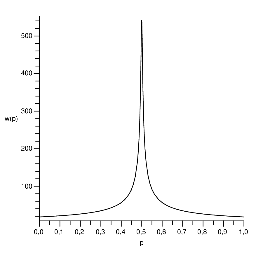
The evaluation of must be conducted with great care to avoid round-off errors. This can be done correctly if the denominator in Eq. (28) is computed as follows: First the polynomial in is expanded and the coefficient of each monomial in is evaluated; secondly, these terms are added up.
In the numerical code, an appropriate test distinguishes which one of these procedures needs to be followed to evaluate an integral. Special care needs to be taken to distinguish between cases 3 and 4. In particular, choice 4 is adopted if the distance between and is below a factor times the distance between and . The factor typically ranges between 4 and 10 and is fixed by setting , with ranging from 0.05 to 0.01.
The evolution of the quasi-geostrophic equation (i.e the case ), as reported in Eq. (4), is computed by projecting the vector field of Eq. (3) over the unitary normal component to the curve at . This means that numerically the first integral on the right hand side of Eq. (28) does not need to be computed (in fact, it is a divergent integral (see [Ro])), since it is a tangential component to the curve at . The second integral on the right hand side of Eq. (28) needs to be projected over the unitary normal component to the curve, and this is easily done. The evolution of the contours for may be indistinctly computed either with Eq. (3) or with Eq. (4).
3.3 A benchmark on the contour integrals
The correctness and accuracy of the numerically computed contour integrals is verified by evaluating for the case in which , and there is only one contour, the circle of radius 1 centred at the origin. This choice is appropriate because it can be compared with the results obtained from the natural parametrization in , i.e. . In this case, the integral to be evaluated is:
which can be numerically evaluated with Maple forcing 15 digits of precision, giving . The exact value of the first component in is zero, which is consistent with Maple forced precision.
The numerical evaluation explained in Section 3.2 has been checked for this one circle case with a number of points along the contour ranging from 100 to 450 and tolerances ranging from 0.05 to 0.01. Errors in the evaluation of extend from (in the less favorable case with 100 points and ) to (in the more favorable case with 450 points and )
The precision of the numerical method thus depends on the number of points on the discretized curve, and also on the tolerance . In our results, we have typically used parameters ensuring accuracy of up to the 5th digit, which is consistent with the 4th order Runge-Kutta method employed to evolve x, and with the precision expected from the redistribution procedure reported in the following subsection.
The numerical method is subjected to further analysis and tests, as discussed in the Results Section.
3.4 The contour evolution
Once in Eq. (27) is conveniently approached, we are ready to apply the 4th order Runge-Kutta method to step forward . At every time step the nodes are redistributed on the contour to guarantee its optimal representation. This means that the numerical method will not track individual trajectories, but rather the whole contour. The relocation of points is performed according to the methodology reported in [DM2], which is reviewed in the Appendix.
3.5 The self-similar problem
The evolution of the self-similar equation (10) may also be computed numerically, since its discrete version may formally be rewritten as:
| (32) |
The numerical evaluation of at each step of the 4th order Runge-Kutta method may be easily achieved with the use of the algorithm developed for the function since it is satisfied that:
where the choice has been considered.
4 Results
The method proposed in Section 3 is used for exploring numerically the solutions of the self-similar equation (10). We first prove the existence of a stationary solution to the self-similar problem by providing its exact expression. This solution is shown to be valid in the range , and is tried as a benchmark of the numerical calculations. Numerical calculations require the selection of specific values of . We systematically explore the results for equal to 0.7 and 0.9. As we have not found any essential differences, we report our findings for = 0.7.